Article

Simultaneous Free Flow and Forcefully Driven Movement of Magma in Lamprophyre Dykes as Indicated by Magnetic Anisotropy: Case Study from the Central Bohemian Dyke Swarm, Czech Republic

Institute of Petrology and Structural Geology, Charles University, Albertov 6, CZ-128 43 Praha, Czech Republic
*
Author to whom correspondence should be addressed.
Geosciences 2019, 9(3), 104; https://doi.org/10.3390/geosciences9030104
Submission received: 27 November 2018 / Revised: 22 January 2019 / Accepted: 21 February 2019 / Published: 27 February 2019
(This article belongs to the Special Issue Advances in the Magnetic Analysis of Geological Processes)

Abstract

:
A composite lamprophyre dyke from the Central Bohemian Dyke Swarm (Czech Republic) shows both indications of magma free flow (normal magnetic fabric with magnetic foliation and lineation parallel to the dyke plane) as well as those of forcefully driven magma movement (intermediate and inverse magnetic fabrics with magnetic foliation perpendicular to the dyke plane). The overall characteristics of the magnetic parameters across the dyke indicate the existence of at least two slightly differing parts that probably represent two magma pulses. The marginal part of the dyke is formed by kersantite, while toward the axial part, the composition gradually changes to spessartite, and obtains an increasing degree of amphibolization. The rocks of the dyke are inhomogeneous, both compositionally and structurally. It is likely that some portions of ascending magma were more viscous than the others, and the magnetic minerals in the more viscous magma portions may have oriented according to their longer dimensions perpendicular to the dyke, creating an inverse fabric. The lengthening perpendicular to the dyke was compensated by the vertical escape of neighboring more fluid magma, creating a normal magnetic fabric. The frequent oblique magnetic fabrics may represent transitions between the above two mechanisms.

1. Introduction

The magnetic fabric of igneous dykes has been intensely investigated because their creation and propagation signify important mechanisms of mass transport within the Earth’s crust and the upper mantle. For example, there are dykes that originated through the almost free flow of magma infilling more or less open fractures in host rocks (close to the surface) as well as dykes that originated through a forceful magma intrusion of the host rocks with no open fractures (in deeper portions of the crust) (see [1]). The structural aspects of these processes have been investigated both from the theoretical and practical points of views (see, for example, [2,3] and references therein). These investigations used various indicators of magma flow, which are unfortunately scarce, and the anisotropy of magnetic susceptibility (AMS), which can be easily measured on almost all types of dyke rocks (e.g., [4,5,6,7,8,9,10,11,12,13,14]).
The different mechanisms of dyke formation are reflected in the type of the preferred orientation of magnetic minerals by grain shape within a dyke, viz. the magnetic fabric. In the free flow of magma within the dyke, the large surfaces of magnetic minerals orient approximately parallel to the dyke, while the longer dimensions orient parallel to the magma flow direction. This type of preferred orientation gives rise to the most common normal (Type I) magnetic fabric [11,12], with magnetic foliation approximately parallel to the dyke plane and magnetic lineation approximately parallel to the dyke plane and to the direction of the flow. In a forceful intrusion, the large surfaces of magnetic minerals orient approximately perpendicular to the dyke, and the longer dimensions orient parallel to the dyke plane [11,15,16], giving rise to the intermediate or Type II magnetic fabric with an approximately perpendicular orientation of magnetic foliation to the dyke plane and magnetic lineation parallel to the dyke [11,12]. In addition, there are two other types of magnetic fabric whose origin is unfortunately less known. One of them is the reverse or inverse (Type III) magnetic fabric with magnetic foliation and magnetic lineation perpendicular to the dyke [10,11,12], the origin of which is attributed to secondary processes such as hydrothermal alteration [12] or to a single-domain effect if the AMS is carried by very small (single domain, SD) magnetic grains [17]. The last type shows almost random orientations of magnetic foliation and lineation, which may result from very complex flow patterns or from severe post-magmatic changes of magnetic minerals [10,18].
The above types of magnetic fabric are assumed to originate in such a way that the dyke walls simply open gradually, and the space between them is infilled by magma. In addition to simple opening, the dyke walls can also be subject to shear movements during dyke formation, with the movements being vertical (dip-slip), horizontal (strike-slip) or even oblique; this process gives rise to more frequent oblique magnetic fabrics (e.g., [7]).
The above magnetic fabric types were most frequently revealed in intermediate and mafic dykes. Much less information is available about magnetic fabric in potassic–lamprophyre dykes (e.g., [19,20]) with source magma generated in the mantle depths (e.g., [21,22,23,24]). Among the potassic–ultrapotassic dykes of the Central Bohemian Dyke Swarm, Hrouda et al. [8] revealed the first three of the above four magnetic fabric types. Interestingly, there is one dyke, the composite lamprophyre dyke near the town of Dobříš, where all three magnetic fabrics can be found: normal in the central part, and intermediate and even inverse magnetic fabrics in the other parts of the dyke. A question arises: how it is possible that the magma movement in one dyke shows indications of both free flow (normal magnetic fabric in central parts) and forceful intrusion (intermediate magnetic fabric in marginal and rim parts)? One explanation of this phenomenon assumes that the central (amphibolized spessartite), marginal (spessartite), and rim (kersantite) parts represent different injections undergoing different mechanisms of magma movement. The other explanation assumes that the dyke originated by one injection within which the petrographical rock types changed gradually to one from another (see [25]), and the rheological state of the moving magma varied accordingly.
In order to evaluate these explanations, new samples were collected along a profile (with dense spacing of 0.5 m in average) across the dyke. They were investigated by standard AMS, which is the anisotropy of the in-phase component of susceptibility (ipAMS), by the anisotropy of the out-of-phase component of susceptibility (opAMS), and by the anisotropy of anhysteretic magnetic remanence (AAMR). The results were combined with detail petrological and geochemical analyses.

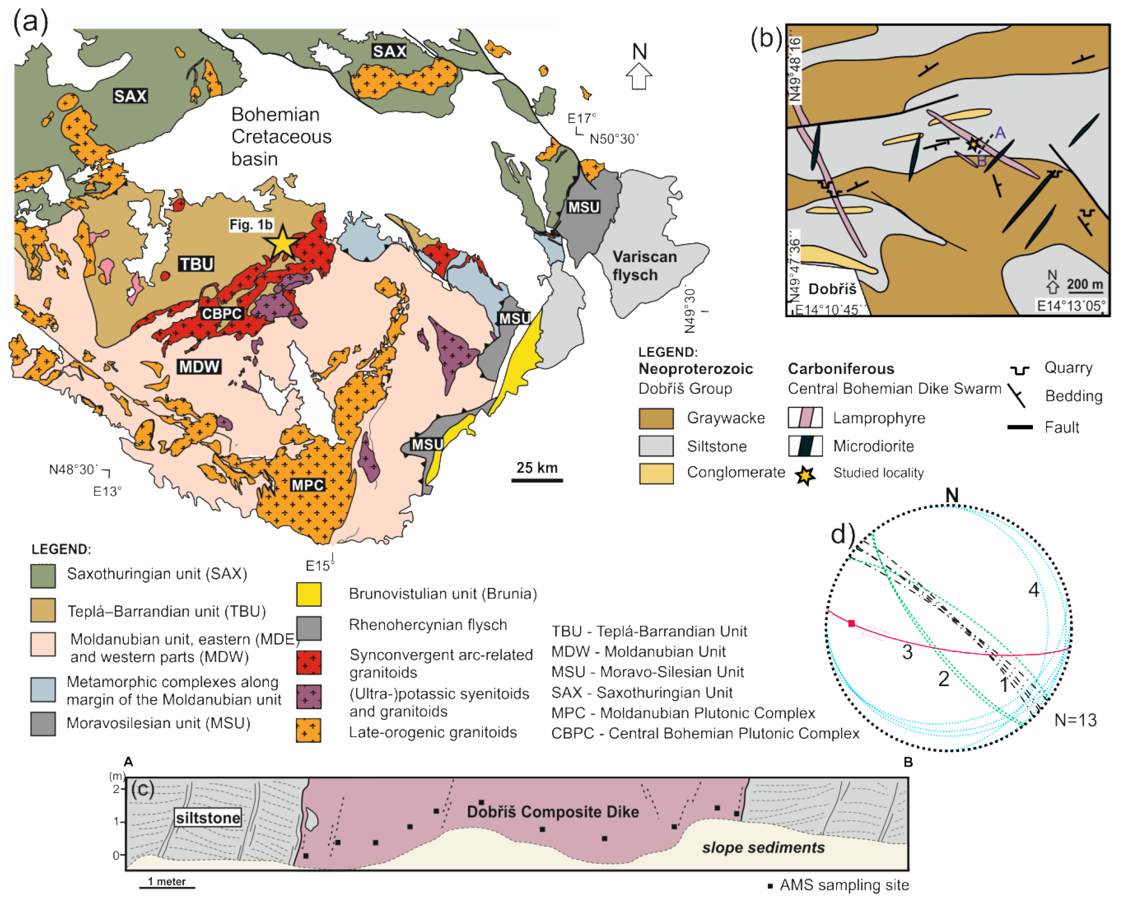
2. Concise Geological Setting

The Bohemian Massif, representing the easternmost segment of the European Variscides, is formed by two crustal blocks (the Brunovistulian and the Teplá–Barrandian, Figure 1) and two zones (the Moldanubian and the Saxothuringian), with rocks affected by various degrees of metamorphism and deformation. The Saxothuringian Zone occupies the northern part of the Bohemian Massif, while the Moldanubian Zone is located in the southeastern part between the Teplá–Barrandian Block in the northwest and the Brunovistulian Block in the east (Figure 1). The Moldanubian Zone is formed by medium-grade (the monotonous and varied units) and high-grade (the Gföhl Unit) metamorphic rocks. The Variscan geodynamic evolution in the Moldanubian Zone was characterized by 380 to 335-Ma long subduction–collision tectonics that resulted in various degrees of metamorphism, magmatic activity, and fast exhumation and cooling (e.g., [26,27,28,29,30]). In general, the overall structure of the Moldanubian Zone is the result of the stacking of several lithotectonic units at ~360 to 345 Ma followed by HT-LP (high temperature, low pressure) metamorphism, anatexis, and late-Variscan wrench tectonics (for a review, see [28,30,31]).
In the Moldanubian Zone, magmatic rocks of Variscan age can be classified into four groups. The first two groups are represented by granitoid complexes that are exposed along two belts, the Central Bohemian Plutonic Complex (CBPC) and the Moldanubian Plutonic Complex (MPC) (Figure 1a). These two complexes differ from each other by age and their relations to Variscan geotectonic processes (e.g., [29,30,32,33,34,35]). The older (c. 355–345 Ma) CBPC straddles the border of the Teplá–Barrandian Block, and is formed by subduction-related calc-alkaline plutons. The younger MPC is composed of peraluminous (S-type) anatectic granitoids (c. 330–300 Ma), and it was formed by extensive migmatitization and isothermal decompression of the surrounding pelitic rocks. The third group is represented by potassic–ultrapotassic rocks (346–337 Ma) that form several isolated plutons (Figure 1a) and dyke swarms [8,36,37,38]. The last group of Variscan igneous rocks have mafic and ultramafic composition (gabbro, norite, troctolite, pyroxenite) and an age of around 340 Ma [39,40,41]. Some of the mafic–ultramafic rocks are unmetamorphosed, but others record amphibolite–granulite facies conditions, and therefore were assumed to be pre-Variscan in age.
The potassic to ultrapotassic rocks form large plutons and dykes having a composition of spessartite, gabbrodiorite, minette, vaugnerite, kersantite, melasyenite, and melagranite. In the western part of the Moldanubian Zone, they are distributed over about a 30 × 100 km area that mostly covers the CBPC (Figure 1a). The dykes have an orientation that is almost E–W and intrudes on not only the basement rocks, but also the granitic rocks of the CBPC. Their thickness varies from five to 20 m, the lengths are often limited to less than one to two km, which is perhaps due to the segmentation of dykes by younger faults. External contacts of porphyry dykes are sharp and generally discordant to folded metamorphic foliations of host gneisses and migmatites.
The studied dyke near Dobříš penetrates the low-grade Neoproterozoic metasediments (slates, metagraywackes, and metasiltstones with thin layers of metaconglomerates). The host rocks belong to the eastern part of the Teplá–Barrandian unit, which was heterogeneously deformed by the ~NW–SE-oriented regional compression during the early stages of Variscan orogeny (for review, see [28,30]). The dyke is about 10 m thick, and has sharply discordant contact, dipping steeply to NNE to NE, in respect to both the regional gently SE dipping bedding and moderately SW dipping cleavage in the host metasiltstones and metagraywackes. A narrow chilled margin (up to 10 cm in thickness) and minor xenoliths of the host rock are present along the contacts. Contact-parallel magmatic foliation (planar preferred orientation of rock-forming minerals) has been identified in some places across the dyke.

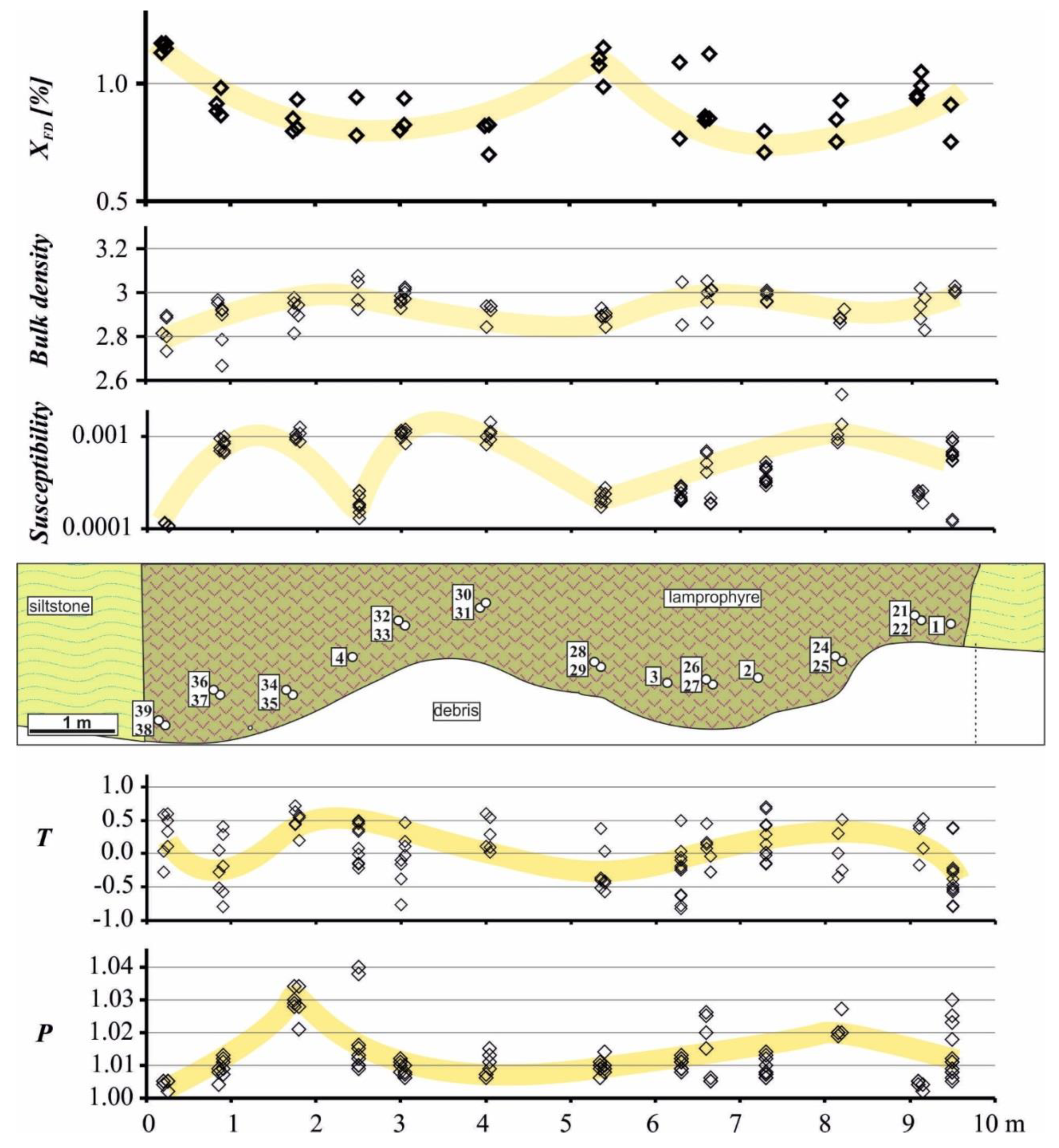
3. Sampling, Technique of Measurement, Data Presentation

Twenty-two oriented samples were drilled across the dyke (Figure 1c) using a portable petrol-powered drilling machine and oriented using a geological compass mounted on a special orientating fixture. From each sample, thin sections for petrological analysis and powder specimen for magnetic mineralogy were made, as well as two to three cylindrical (25 mm in diameter and 21–22 mm in height) specimens for magnetic anisotropy measurement. The standard AMS (ipAMS) and the opAMS were measured with the KLY-5 Kappabridge [42] using the three-dimensional (3D) rotator [43], and computed by the SAFYR (ver. 6) program. The AAMR was measured using the LDA-5 anhysteretic magnetizer/AF Demagnetizer and JR-6A Spinner Magnetometer (both produced by Agico Inc. Brno). The bias field was 500 μT, and the AF field was 40 mT; before anhysteretic magnetizing in each direction, the specimen was tumble AF demagnetized in the field of 50 A/m. The measurement was processed using the program REMA (ver. 6.20, M. Chadima) based on the theory by Jelínek [44].
Until now, the dominant method for measuring the AMS of rocks is that of an induction bridge, which measures the susceptibility and its anisotropy in an alternating magnetic field. The susceptibility that is measured in this way can in general be resolved into a component that is in-phase with the magnetizing field, and a component that is out-of-phase. The standard AMS is in fact the anisotropy of the in-phase component (ipAMS). The technique for measuring the anisotropy of the out-of-phase component (opAMS) was developed only recently [42].
The mean bulk susceptibility, eccentricity, and shape of the anisotropy ellipsoid can be characterized by the following parameters [45,46]:
Km = (k1 + k2 + k3)/3
P = k1/k3
T = (2 η2η1η3)/(η1η3) = 2 ln F/ln P − 1
where k1k2k3 are the principal values, and η1 = ln k1, η2 = ln k2, and η3 = ln k3. The parameter P, which is called the degree of anisotropy, indicates the intensity of the preferred orientation of the magnetic minerals in a rock. The parameter T characterizes the shape of the anisotropy ellipsoid. If 0 < T < +1, the ellipsoid is oblate (the magnetic fabric is planar); T = +1 means that the ellipsoid is rotationally symmetric (uniaxial oblate). If –1 < T < 0, the ellipsoid is prolate (the magnetic fabric is linear); T = –1 means that the ellipsoid is uniaxial prolate.
In order to obtain a statistical evaluation of the AMS/AAMR at individual localities, the ANISOFT package of programs [47,48,49] was used, which enable a complete statistical evaluation of a group of specimens. The orientations of magnetic foliations and magnetic lineations, the respective mean directions, and the corresponding confidence areas are presented in equal-area projections on the lower hemisphere in the dyke coordinate system (the dyke was rotated about its strike to a vertical position, and about the vertical axis to the N–S position).
The magnetic minerals carrying the rock magnetism were investigated through the method of the maximum theoretical paramagnetic susceptibility (MTPS, see [50]), using the susceptibility variation with the magnetizing field, the operating frequency, and the temperature. The susceptibility variation with magnetizing field was measured in the fields ranging from five A/m to 700 A/m at the operating frequency 1220 Hz using the automated mode of the KLY-5 Kappabridge. The variation can be concisely characterized by the Vm parameter defined as follows [51]:
Vm = 100(kmaxkmin)/kmin [%]
where kmax and kmin are the maximum and minimum susceptibilities, respectively, that were obtained during one measuring run. The susceptibility variation with operating frequency was investigated at the frequencies 976 Hz and 15,616 Hz in the driving field of 200 A/m using the MFK1-FA Kappabridge. It can be represented quantitatively by the commonly accepted percentage loss of susceptibility [52]:
XFD = 100(kLFkHF)/kLF [%]
where kLF and kHF are susceptibilities measured at low and high frequencies, respectively. The low and high frequencies were 976 Hz and 15,616 Hz. The susceptibility variation with temperature was measured on coarsely powdered pilot specimens in temperature intervals between −194 °C and 0 °C and between 25–700 °C using the CS-L Cryostat, CS-4 Furnace [53], and the MFK1-FA Kappabridge. The susceptibility versus temperature curve that is measured between −194 °C and 700 °C is called the heating curve, while the curve measured between 40–700 °C is called the cooling curve. The high-temperature curves were measured in the atmosphere of flowing argon (10 l/min). The Curie temperatures were determined using the Petrovský and Kapička [54] method based on searching for the beginning of the paramagnetic hyperbola just at the Curie temperature.
The bulk rock density was determined through simply measuring the dimensions of cylindrical specimens for measuring the AMS using vernier and weighing the specimens using analytical scales.

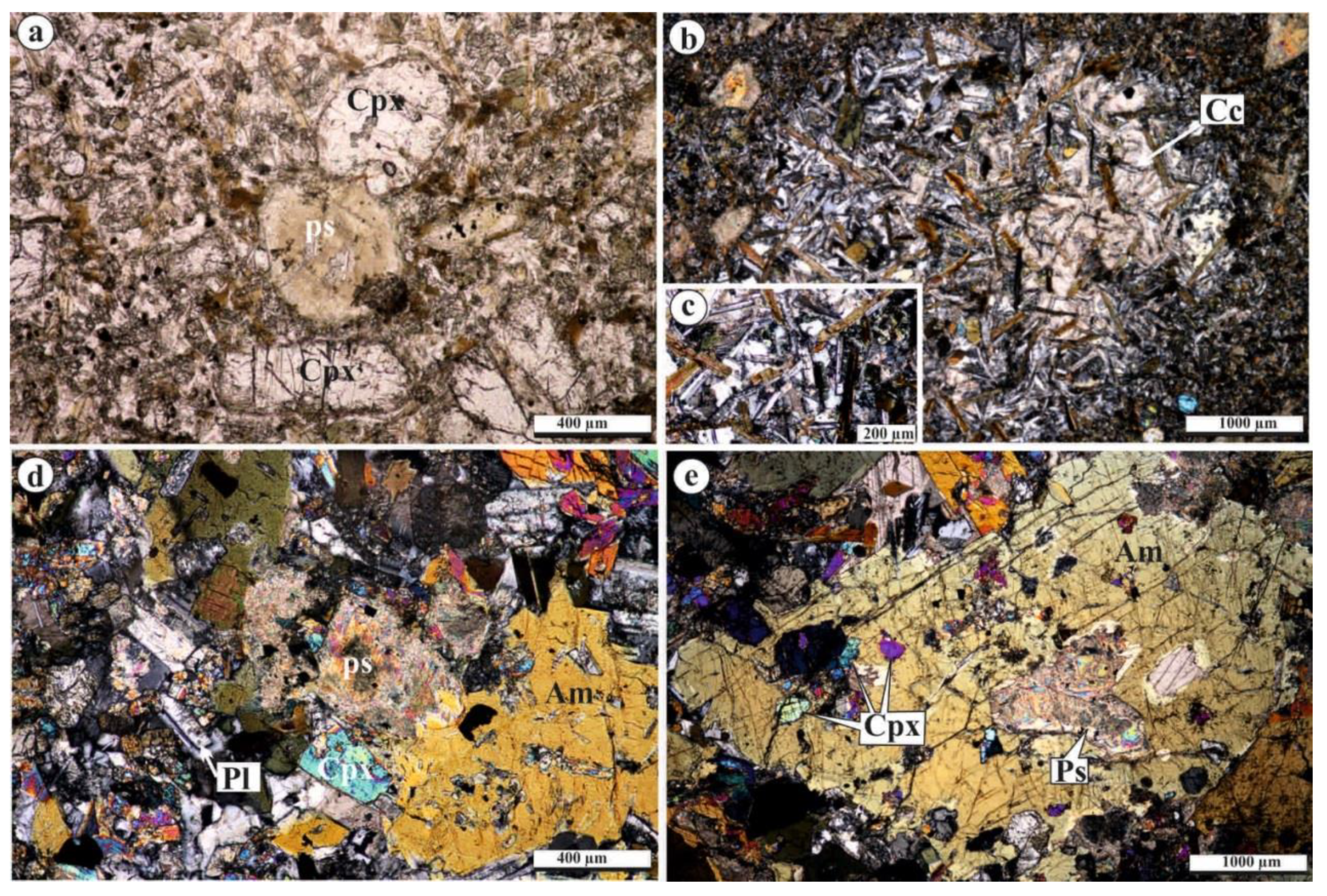
4. Petrology and Bulk Rock Chemistry

Modal contents of minerals and their textures show a gradual change from the rim to the central part of the dyke. After Holub [25], the dyke is formed by kersantite (plagioclase > K-feldspar with high biotite content) upon contact with the host siltstone, and by hornblendite in the axial part of the dyke. The bulk rock composition of three main varieties is given in Table 1. It should be noted that the different composition and mineral mode is partially due to the degree of amphibolization (see later). Both axial and rim parts are separated by a thin zone of spessartite (plagioclase > K-feldspar with high amphibole content). The dyke margin, up to several cm from contact with the host rocks, consists of a very fine-grained (<0.15 mm) matrix with phenocrysts (up to 1.5 mm) of clinopyroxene and pseudomorphs of talc after olivine (Figure 2a). The minerals that are present in the matrix are plagioclase > biotite > clinopyroxene, and small amounts of amphibole, K-feldspar, quartz, carbonate, magnetite, and sulphides. The amphibole content increases toward the central part of the dyke, and the biotite content is about 8 vol%. The pseudomorphs of talc after olivine instead of orthopyroxene are assumed by their shapes and comparison with other lamprophyre dykes with similar phenomena of olivine replacement to talc [38]. In addition to talc, the pseudomorphs contain accessory amounts of quartz and Cr-spinel. The phenocrysts of clinopyroxene may contain inclusions of apatite and opaque minerals. A striking feature of this part of the rock is the presence of multiphase ocelli (1.55–4.5 mm), which are formed by tabular grains (<0.5 mm in size) of plagioclase and brown biotite with small amounts of green amphibole and a smaller amount of K-feldspar (Figure 2b). The minerals in the ocelli show random orientation (Figure 2b,c). Some ocelli contain also carbonate and minor quartz.
Farther from the dyke rim, the rock gradually becomes coarse-grained. Although the matrix phases can have a size of up 0.4 mm, the coarsening is mainly due to amphibole grains (up to 1.5 mm in size) that overgrow or enclose clinopyroxene and pseudomorphs after olivine (Figure 2d). It has a brown color that transitions to green rims. In contrast to the contact zone, biotite content decreases (<1 vol%), and that of amphibole increases (up 60 vol%). The amounts of clinopyroxene phenocrysts and talc pseudomorphs also decrease due to their replacement by amphibole. Matrix minerals are similar to those from the contact zone and consist of plagioclase, amphibole, K-feldspar, clinopyroxene, biotite, and minor quartz and carbonate.
The axial part of the dyke is coarse-grained and consists mostly of amphiboles that reach a grain size of up to five mm (Figure 2e). Biotite is not present, or can occur as an accessory phase. Amphibole contains relics of clinopyroxene, talc pseudomorphs, and encloses plagioclase. The original matrix is locally preserved and consists of amphibole, clinopyroxene, plagioclase, minor carbonate, and quartz.
No significant variation in the composition of minerals was observed between the rim and central parts of the dyke. Clinopyroxene is augite to diopside (XMg = 81.58−87.50 mol %). Amphibole corresponds to tschermakite, magnesio-hornblende, magnesio-hastingstite, and edenite in composition. Its Mg (XMg = Mg/(Mg + Fe2+)) ratios slightly increase from the marginal part of the dyke (0.63–0.72) to the central part (0.67–0.86). Some amphibole grains in the central part are replaced along the rims by actinolite. Biotite has XMg = 0.55−0.65, but rarely, phlogopite (0.70–0.72 XMg) is also present. Plagioclase is zoned, and shows a wide compositional range, from andesine-labradorite (37.80–69.83% An) in the marginal part of the dyke to andesine-bytownite (31.16–85.34% An) in the central part of the dyke. K-feldspar is orthoclase with 72.30–76.74% Or and a mixture of celsian (1.89–3.82% Cn).
In addition to a fast-cooled matrix and the presence of ocelli textures at the contact zone, the main difference between the rim and central part of the dyke is related to the presence and amounts of biotite and amphibole. Biotite with high XMg content could represent the original phase, but it is not clear whether some amphibole was also formed among the early crystallized phases. As shown above, amphibole is a late crystallized phase, and it clearly replaces or overgrows the early crystallized minerals (plagioclase, clinopyroxene, and olivine). Based on the original minerals, the rim part corresponds to kersantite, which is consistent with the findings of Holub [25], but the central part is represented by spessartite, with an inward increase of amphibolization degrees. Bulk rock chemistry indicates that the central part has less silica, aluminum, and potassiumm but higher amounts of MgO and CaO. Calculated normative contents of minerals reveal that the rim part has higher content of plagioclase, orthoclase, and hypersthene, but lower amounts of diopside and olivine compared to the central part. As shown above, the pseudomorphs are after olivine, but the presence of small amounts of orthopyroxene among the primary phases is not excluded. In addition, some Ca could be incorporated into the original carbonate.

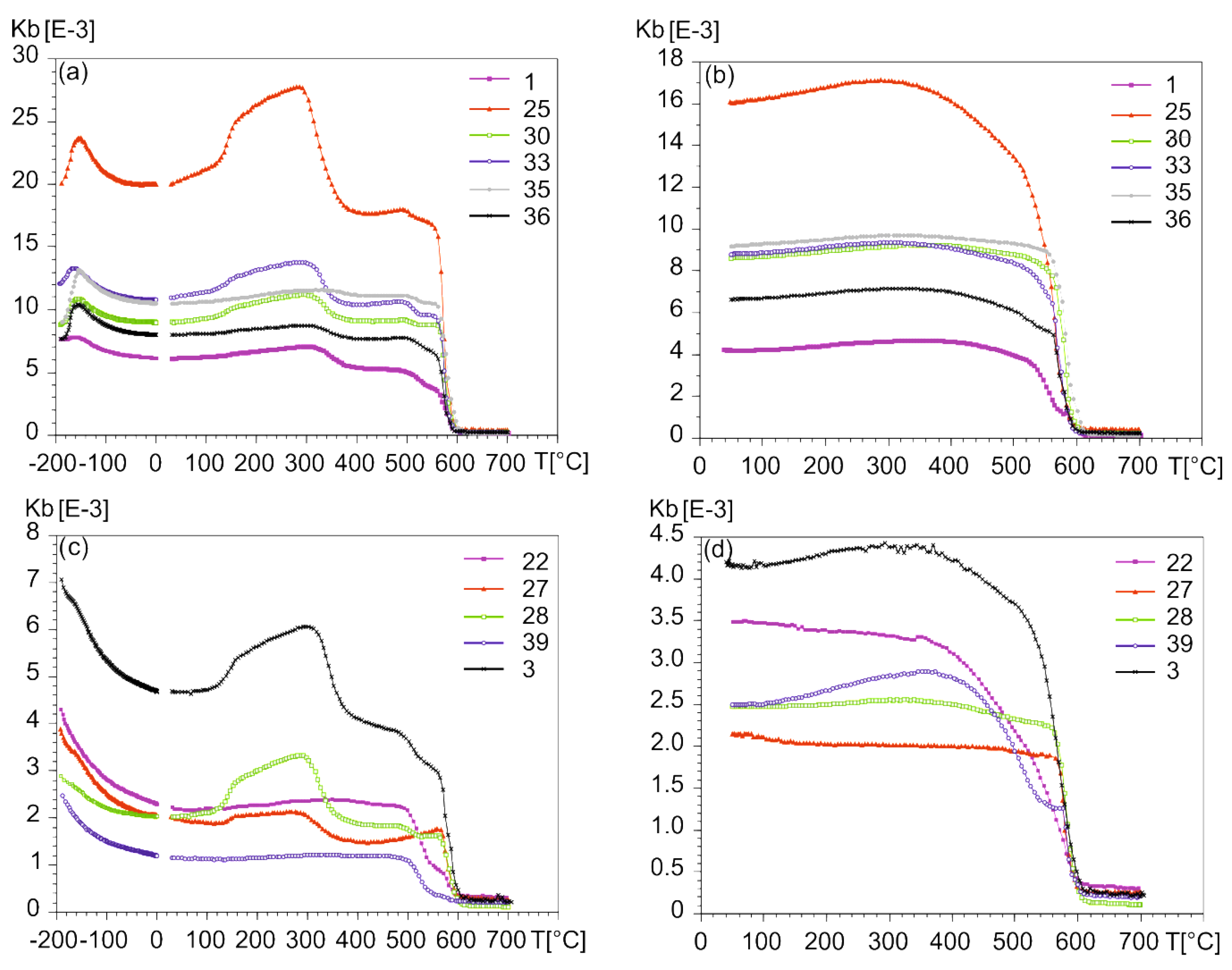
5. Magnetic Mineralogy

The mean volume susceptibility of the Dobříš dyke is moderate, covering the entire order of 10−3 (Figure 3). The MTPS method, which calculates the rock paramagnetic susceptibility from the Fe and Mn contents obtained from the whole-rock chemical analyses (see [50]), shows that the contribution of paramagnetic minerals to the whole-rock susceptibility is an order of magnitude lower: about 0.6 × 10⁻³. Consequently, the rock’s susceptibility is dominantly carried by ferromagnetic minerals (encompassing ferrimagnetic, antiferromagnetic, and ferromagnetic sensu stricto ones).
The variation of susceptibility with temperature was investigated on 11 pilot specimens that cover all rock types in the dyke. The susceptibility versus temperature curves of the high-temperature segment (between room temperature and 700 °C) mostly show three susceptibility decreases in the heating curves: one between 300–360 °C, the second between 495–515 °C, and the third between 570–590 °C (Figure 4a,c). The last temperature probably indicates magnetite, the other two may indicate Fe–Ti oxides with different contents of Ti. The hump of susceptibility between ca. 150–350 °C can be ascribed to a new phase that may have been created during specimen heating. It should be emphasized that the curves of all the specimens are similar, even though they come from different positions within the dyke and represent different rock types, thus supporting gradual inward changes in mineral and bulk rock chemistry within the dyke. The cooling curves run lower than the heating ones and show only one susceptibility decrease, i.e., that at 570–590 °C (Figure 4b,d). This probably indicates the dissolution of the earlier separated phases, resulting in the creation of one phase.
The low-temperature curves (between −190 °C and 0 °C) show susceptibility decreases at −160 °C and −170 °C at the Verwey transition, which is typical of relatively pure magnetite [55], in six specimens, and paramagnetic hyperbola in five specimens (Figure 4a,c).
In specimens that showed no Verwey transition, but indicated the existence of paramagnetic hyperbola, the low-temperature segments of the curves were resolved into paramagnetic hyperbola and a ferromagnetic straight line using the method by Hrouda [56]. This technique revealed that the paramagnetic susceptibilities are mostly in the order of 10−4, thus indicating that the rock’s susceptibility is even in such cases dominantly carried by ferromagnetic minerals (magnetite).
The variation of in-phase susceptibility with field is very weak, with the K/Kmin ratio being less than 1.02 (Figure 5a). Among ferromagnetic minerals, pure magnetite shows virtually field-independent susceptibility, while in titanomagnetite, pyrrhotite, and hematite, the susceptibility may be clearly field-dependent, even in low fields that are commonly used in AMS meters [51,57,58,59,60,61,62]. From this point of view, the weak in-phase susceptibility variation of most of the investigated specimens probably indicates the presence of only slightly impure magnetite or very low amounts of titanomagnetites.
The out-of-phase susceptibility is about two orders lower than the in-phase susceptibility. To visualize its variation with field, the K–Kmin difference is used instead of the K/Kmin ratio to avoid problems with normalizing by very low numbers. Nevertheless, it clearly shows an observable increase with field (Figure 5b). As the out-of-phase susceptibility of pure magnetite is effectively zero, while it is clearly non-zero in titanomagnetite, pyrrhotite, and hematite (see [63]), the low, but non-zero, out-of-phase susceptibility probably indicates the presence of either impure magnetite or very low amounts of titanomagnetite.
The grain size of ferromagnetic minerals can be assessed, at least partially, through frequency-dependent susceptibility. Namely, the frequency-dependent susceptibility is effectively zero in multi-domain (MD) and single-domain (SD) grains of magnetite (titanomagnetite) as well as in its ultrafine superparamagnetic (SP) grains (e.g., [51,64]). On the other hand, it can be clearly non-zero in magnetically viscous grains that are transitioning from the SP state to the SD state. The values of the XFD parameter characterizing the frequency-dependent susceptibility quantitatively are low, mostly lower than 1% (see Figure 3), approaching the detection limit of the method [65]. Consequently, the investigated dyke contains very low amounts of magnetically viscous grains, if any.
It can be concluded that the dominant carrier of the ipAMS is magnetite, even though some other magnetic phases are also present. As the AMS of magnetite is controlled by its grain shape, the rock ipAMS is controlled by the preferred orientation of magnetite by grain shape. The opAMS is controlled either by impure magnetite of very low amounts of titanomagnetite. The AAMR in the measuring configuration used (without using magnetization/demagnetization windows) is controlled by the mineral(s) that can be easily magnetized anhysteretically and subsequently demagnetized before changing the magnetizing direction, which is probably represented by low-Ti titanomagnetite.

6. Magnetic Fabric

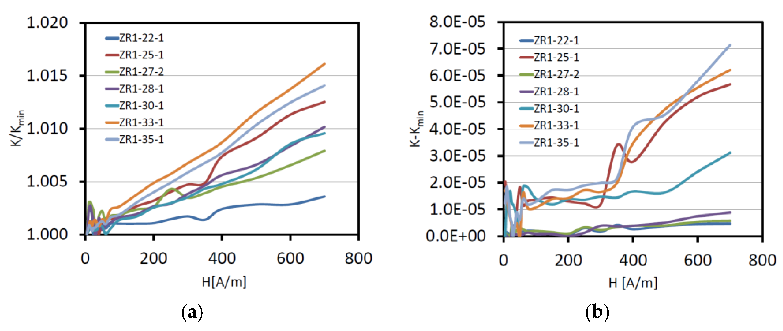
6.1. Standard Anisotropy of Magnetic Susceptibility (AMS)

The degree of AMS is very low, mostly about P ~1.01, and reaching P = 1.04 (Figure 3). The shape of the AMS ellipsoid ranges from very prolate to moderately oblate (Figure 3). Both the magnetic foliations and lineations are relatively well defined. From the point of view of the orientations of magnetic foliations and magnetic lineations with respect to the dyke plane, the dyke can be divided into seven domains showing different, but relatively homogeneous, orientations. In two domains, D1 (samples 34 and 35) and D2 (samples 3, 28, and 29), the magnetic foliation is approximately parallel to the dyke plane, while the magnetic lineation is horizontal and also parallel to the dyke plane (Figure 6); this fabric can be denoted as normal or Type Ia. In domain D3 (samples 4 and 30), the magnetic foliation is almost perfectly vertical and perpendicular to the dyke, and the magnetic lineation is also mostly perpendicular to the dyke (Figure 6). This fabric type is no doubt inverse or Type IIIb. In domain D4 (samples 2, 24–27), the magnetic foliation is mostly perpendicular to the dyke, varying in the dip from horizontal to vertical, and magnetic lineation is mostly horizontal, perpendicular to the dyke (Figure 6). This magnetic fabric can be also denoted as inverse, transitioning from Type IIIa to IIIb. In the domains D5 (samples 36–39), D6 (samples 31–33), and D7 (samples 1, 21, 22), both the magnetic foliations and magnetic lineations are oblique with respect to the dyke plane (Figure 6), and the magnetic fabrics cannot be described in simple terms such as normal or inverse. It is likely that the rocks in these domains suffered local strike-slip movements that rotated the magnetic fabrics.

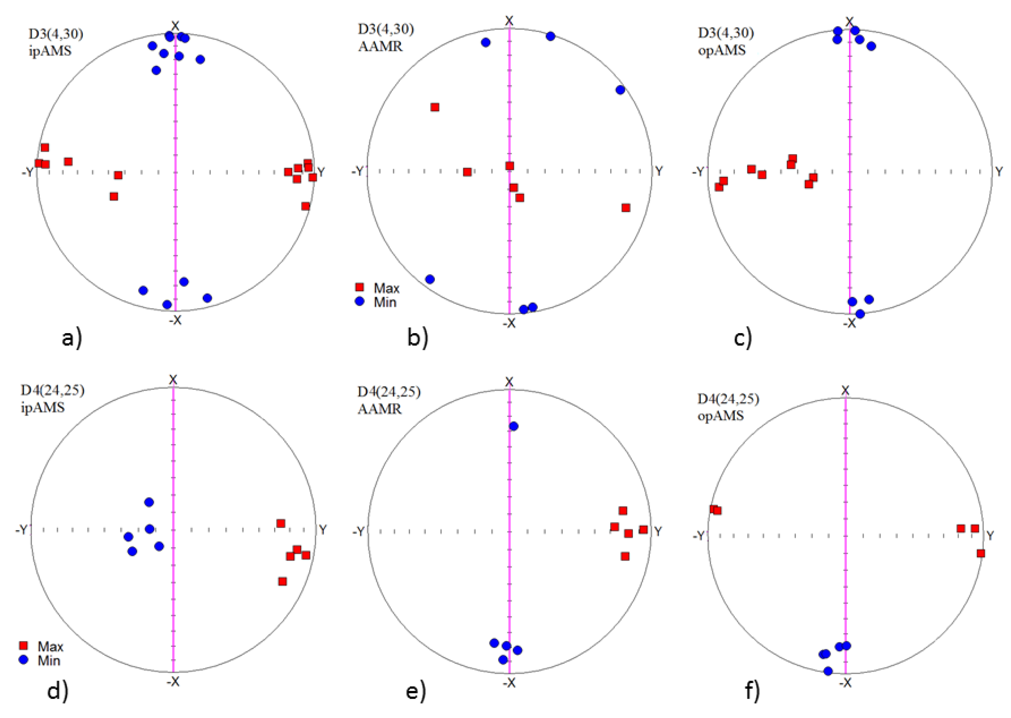
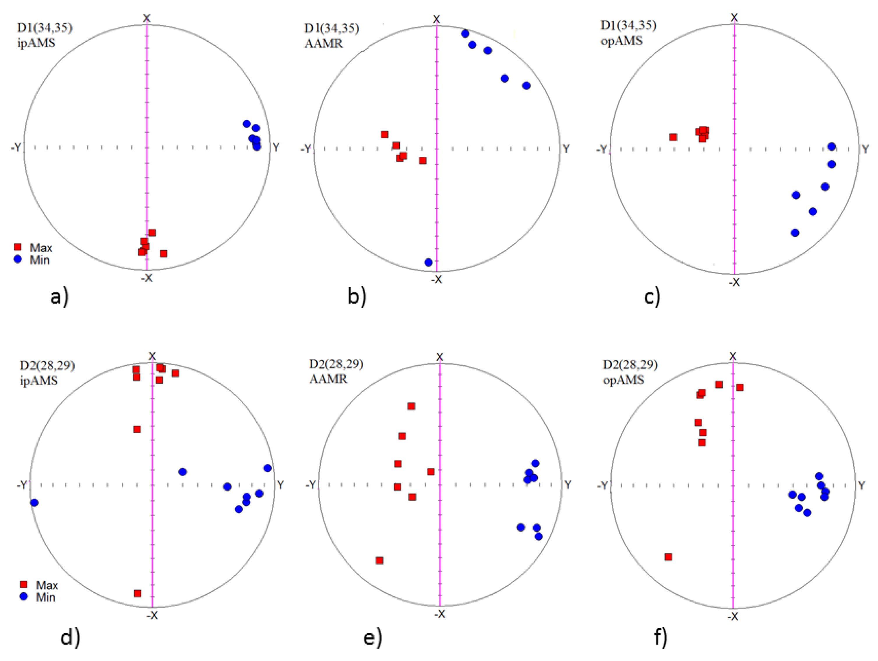
6.2. Anisotropy of Anhysteretic Magnetic Remanence (AAMR) and Anisotropy of Out-of-Phase Magnetic Susceptibility (opAMS)

The reason for investigating the AAMR was to find out whether the inverse AMS fabric results from the perpendicular orientation of larger dimensions of magnetic minerals with respect to the dyke plane or from the grains of magnetic minerals being very small and SD in state. Namely, as shown by Potter and Stephenson [66] for example, the maximum susceptibility is along the maximum dimension in the MD particle, while it is along the minimum dimension in the SD particle. The minimum susceptibility is along the minimum dimension in the MD particle and along the maximum dimension in the SD particle. As the measurement of AAMR is an order-of-magnitude more laborious and time-consuming than that of AMS, the AAMR was not measured in all the available specimens, but preferably in a selection of those coming from domains with normal (domains D1, D2) and inverse (domains D3, D4) AMS fabrics.
In both the domains showing normal ipAMS fabric (D1, D2), the ipAMS foliation and ipAMS lineation are parallel to the dyke plane; the latter is horizontal (Figure 7a,d). The AAMR and opAMS foliations are parallel to the dyke in the D2 domain, while they deflect azimuthally from the dyke in the D1 domain; the AAMR and opAMS lineations are very steep in the D1 domain and gentle to very steep in the D2 domain (Figure 7b,c,e,f).
In both the domains with inverse AMS fabric (D3, D4), the ipAMS foliation is perpendicular to the dyke plane, being horizontal in the D4 domain and vertical in the D3 domain; meanwhile, the ipAMS lineation is perpendicular to the dyke (Figure 8a,d). The AAMR foliations are very steep, and mostly perpendicular to the dyke; the AAMR lineations are perpendicular to the dyke and horizontal in the D4 domain, and mostly parallel to the dyke and vertical in the D3 domain (Figure 8b,e). The opAMS foliations are vertical and perpendicular to the dyke in both domains, and the opAMS lineations are horizontal and perpendicular to the dyke in the D4 domain, and show a variable plunge within the vertical plane perpendicular to the dyke in the domain D3 (Figure 8c,f).
In summary, the ipAMS foliation poles are not parallel to the AAMR lineations as well as the ipAMS lineations are not parallel to the AAMR foliation poles in any domain. In addition, the frequency-dependent susceptibility is very low (mostly XFD < 1%), indicating that the ultrafine magnetically viscous particles in transition from the SP state to the SD state are present in very low amounts. Assuming continuous grain-size distribution from SP through SD to MD, and realizing that the susceptibility of SD particles is lower than that of MD or SP particles, the very low values of the XFD parameter may indicate that the SD particles are not abundant enough to dominate the rock magnetism. One can conclude that the inverse AMS fabrics are very unlikely due to the dominance of SD particles, and their existence should be ascribed to specific mechanisms in detailed magma movement.
The magnetism of the dyke is dominantly carried by MD ferromagnetic minerals. If different subpopulations of those minerals had similar geological histories, one would expect coaxial orientations of ipAMS, AAMR, and opAMS. However, this is true only partially. The ipAMS, AAMR, and opAMS foliations and lineations all show moderate to large differences. These may be ascribed to slightly different subpopulations of magnetic grains controlling the individual anisotropies. They may reflect a transition from vertical feeding flow to horizontal flow, representing advanced magma propagation.
In the D1 and D2 domains, in which the ipAMS, AAMR, and ipAMS fabrics can be classified as normal, all the three magnetic fabrics evidently indicate relatively free flow, during which the magnetic minerals orient parallel, with their larger surfaces to the dyke, and with their longer dimensions probably parallel to the magma flow. The titanomagnetite longer axes, being oblique to vertical as indicated by AARM and opAMS lineations, probably represent the direction of the feeding flow of the dyke. The horizontal longer axes of magnetite indicated by ipAMS probably represent the advanced magma propagation along the dyke. We hypothesize that the magnetic minerals crystallized only during magma feeding a joint and creating the dyke. Then, the titanomagnetites crystallized earlier at higher temperatures than magnetite.
In the D3 and D4 domains, whose ipAMS, AAMR, and ipAMS fabrics can be classified as inverse, the magnetic minerals are oriented with their larger surfaces perpendicular to the dyke and with their longer dimensions also perpendicular to the dyke. Such a magnetic fabric may have originated as follows. The magma movement is no longer represented by free flow. Rather, it is akin to forceful injection when the later magma batches push on the earlier ones. In this process, the larger surfaces as well as the longer axes of magnetic minerals orient perpendicular to the compression direction. It is interesting that in the D4 domain, the ipAMS foliations, although perpendicular to the dyke, are horizontal, while the AAMR and opAMS foliations are also perpendicular to the dyke, but vertical. This would mean that titanomagnetites indicate horizontal compression along the dyke, while the magnetite indicates vertical compression.

7. Discussion

7.1. Variation of Mineral Textures and AMS Fabrics across the Composite Dyke

As shown above, the dyke at Dobříš is represented by various domains differing in composition and fabrics. Its compositional change from kersantite occurring mostly at the margin parts to spessartite in the central part is accompanied by an increase in the degrees of amphibolization. This inward transition is gradual, and can be seen in the grain sizes of minerals, mainly of amphibole, with its high volume content in the central part. It seems that the original magma of kersantite composition intruded into a relatively cold environment, making chilled contacts with the host siltstone. Although phenocrysts of clinopyroxene and talc pseudomorphs reach sizes of up to 1.5 mm, the rock still has a fine-grained matrix. The continuous change in grain size, modal amounts of original mineral (biotite), mineral composition (plagioclase, XMg values of clinopyroxene), and bulk rock composition suggest a gradual change of the source magma to spessartite, which intruded through the central part of the dyke. Based on the early crystallized minerals, both magmas were generated by partial mantle melting, but kersantite melt came from the mica-bearing peridotite part [38]. The presence of spectacular ocelli textures at areas in contact with the rim suggests that the bubbles were filled at high temperature by infiltration of the residual melt from the matrix, which crystallized into plagioclase, biotite, amphibole, and quartz, with or without calcite. As there is no sharp boundary between kersantite and spessartite, the more mafic magma penetrated the axial part of the dyke in the still relatively warm environment formed by kersantite. Consistent with textural relations, amphibole was formed during the last stage of crystallization. The presence of amphibole enclosing both phenocrysts and matrix minerals suggests that it formed in subsolidus conditions after the emplacement of the dyke. The assumption about high temperature being sufficient for amphibole formation of magnesio-hornblende and tschermakite composition is supported by the ocelli textures filled by plagioclase, amphibole, and biotite.
As illustrated in Figure 3, except for the percentage loss of susceptibility (XFD), the values of bulk density, mean susceptibility, shape parameter (T), and degree of AMS (P) show generally bimodal distribution and divide the dyke into two NE and SW segments. Each segment is characterized by an elevated central part and depressions at the marginal parts. The values of the XFD parameter are roughly inverted to those of the above parameters. This bimodal distribution of magnetic parameters implies that the dyke was formed by two magma pulses: one creating the NE segment, and the other creating the SW one. Based on the results of petrology, the two pulses do not represent timely and mechanically separated magma batches, but rather represent the gradual development of one slowly moving magma, changing its composition from kersantite to spessartite.

7.2. Implications of AMS Fabrics to Multistage Evolution of Magmatic Dykes

Several theoretical models of the dyke formation can be basically considered. They either assume that the dyke walls simply open gradually and the space between them is infilled by magma, or they also consider that during dyke formation, the dyke walls are subject to shear movements, which can be vertical (dip-slip), horizontal (strike-slip), or even oblique. The moving magma is supposed to resemble the flow of the Newtonian or Binghamian liquid or a transition between these two (e.g., [7]). The magma movement is advantageously described in terms of intrusive strain; four different cases (models 1–4 in Figure 9 and Figure 10) can occur. The predicted orientations of the magnetic foliations and lineations are obtained from our own program based on the line/plane and viscous models (for details, see [67,68]).
Model 1 (Figure 9) considers that a vertical dyke opens without the transcurrent component being fed with vertically flowing magma, resembling the Newtonian liquid (Figure 9a,b). The AMS ellipsoid is nearly neutral, and the magnetic foliation is very steep, striking parallel to the dyke wall and dipping toward the wall; the magnetic lineation is also very steep, being roughly parallel to the dip of the magnetic foliation (Figure 9f). This magnetic fabric can be classified as normal. In the tip parts of the dyke (Figure 9b), the magma movement resembles pure shear, the AMS ellipsoid is predominantly oblate, and the magnetic foliation and magnetic lineation are roughly horizontal, making them perpendicular to the dyke, and creating the intermediate magnetic fabric (Figure 9g) [7]. If the uppermost part of the dyke does not open sufficiently rapidly, the flow direction may change to horizontal (Figure 9c); as a result, the magnetic foliation orients near the dyke walls, and the magnetic lineation becomes horizontal (Figure 9h). If the horizontal flow is no longer possible for mechanical reasons, the magnetic foliation and magnetic lineation also may become vertical (Figure 9i). If the magma flow resembles the Binghamian liquid (Figure 9e), the magnetic foliation is parallel to the dyke walls, and the magnetic lineation is vertical (Figure 9j).
Model 2 (Figure 10a–e) assumes that a vertical dyke is vertically fed with magma, and the dyke walls move in a dip-slip way (Figure 10a). In the marginal areas, the basic orientations of magnetic foliation and magnetic lineation remain steep (Figure 10b). In the tip areas, the magnetic foliation deflects from the horizontal position, and the magnetic lineation remains more or less horizontal (Figure 10c). If the magma movement changes to horizontal, while the wall movements remain dip-slip oriented, the magnetic foliation may slightly deflect from the vertical, and the magnetic lineation may remain more or less horizontal if the shear movement is weak, or more or less vertical if the shear movement is relatively strong (Figure 10d). If the magma feeding magnetic foliation is vertical and oriented in a perpendicular way to the dyke, the magnetic lineation deflects from the vertical due to dip-slip movements, and the magnetic foliation does not substantially change its orientation (Figure 10e).
Model 3 (Figure 10f–j) assumes the same dyke, but with its walls making a strike-slip movement (Figure 10f). In the marginal parts, the magnetic foliation gradually deflects from the approximate parallelism to the dyke toward the perpendicularity to the dyke, and the magnetic lineation moves along the great circle from the vertical toward the horizontal (Figure 10g). In the tip parts, the magnetic foliation remains nearly horizontal, and the magnetic lineation gradually deflects from the dyke strike direction (Figure 10h). If the magma feeding direction is horizontal, the magnetic foliation remains more or less vertical, but deflects azimuthally from the dyke plane; the magnetic lineation remains nearly horizontal and rotates azimuthally from the dyke strike (Figure 10i). If the magma feeding magnetic foliation is vertical and oriented in a perpendicular way to the dyke, the magnetic lineation remains more or less vertical, and the magnetic foliation rotates azimuthally due to strike-slip movements (Figure 10j).
Model 4 (Figure 10k–o) considers the same dyke, but with its walls performing oblique shear movements (Figure 10k). In this case, the magnetic foliation and lineation show movements, combining the previous three models.
Based on the above outlined analysis on magma flow within dykes (with or without shear movements of the walls), the magnetic fabrics in different parts of the Dobříš dyke indicate analogies with some model types in Figure 9 and Figure 10. For example, the ipAMS fabrics in the D1 (Figure 7a) and D2 (Figure 7d) domains correspond to model 1 (Figure 9c,h), and those in the D5 and D6 domains (Figure 6) correspond to model 3 in Figure 10g,i,j, respectively. The AAMR fabric in the D1 domain (Figure 10b) is similar to that in model 3 (Figure 10j), and the fabric in the D2 domain (Figure 7e) corresponds to that of model 1 (Figure 9a). There is also an additional type showing both magnetic foliation and magnetic lineation perpendicular to the dyke, which is represented by the D3 domain (Figure 8a) and the D4 domain (Figure 8d). All this indicates that the magma movement must have been very complex.
Even though the magnetic fabric in the Dobříš dyke shows features in some domains that can be due to shear movements (corresponding to models 2 and 3), we cannot find the effects of these movements on the whole dyke. In our opinion, the above features are due to small-scale shear movements within the dyke, rather than overall dyke wall movements.
As indicated in Figure 6, the orientations of magnetic foliation poles and magnetic lineations across the dyke can be classified into seven domains (Figure 11). The two domains (D1, D2) with normal fabrics (magnetic foliation parallel to the dyke plane) are in contact with the D3 and D4 domains, which have inverse fabrics (magnetic foliation and lineation perpendicular to the dyke plane). The domains D5 and D7 with mixed fabrics between normal and inverse are located in areas in contact with surrounding siltstone, while the D6 domain, which has similar fabrics, is located in the central part of the dyke. The detailed textural relations and bulk rock chemistry of the rocks in domain D5 indicate that its composition is kersantite, and that it intruded first into the cold surrounding environment. We also showed that the formation of the dyke was evolved toward the central part, where new magma of more mafic composition intruded. Therefore, the fabrics of the marginal domains (D5 and D7) were controlled both by friction with the wall of the host siltstone, and by the movement of ascending magma.
Although the degrees of amphibolization and coarsening of the rocks increase inward, the original texture and bulk rock chemistry is not uniform in the central part of the dyke. This suggests that the whole dyke was fed by different portions of melt that intruded in different time intervals that were close to each other. The presence of the D6 domain with mixed magnetic fabrics in the central part of the dyke can be explained by reopening of the dyke on both sides of the D6 domain, where two normal and inverse domains occur. We assume that the D1 and D2 domains with vertical magnetic fabrics represent the younger portions of melt that penetrated the dyke after the D3 and D4 domains were partly solidified. Consequently, the magnetic minerals in the more viscous magma portions may have oriented by their longer dimensions perpendicular to the dyke, because the lengthening perpendicular to the dyke was compensated by the vertical escape of neighboring, less viscous magma.
The investigated dyke at Dobříš shows a rare phenomenon, viz. the occurrence of both normal and inverse magnetic fabrics within one dyke. The question arises of how it is possible that the magma movement in one dyke shows indications of both free flow (normal magnetic fabric) and forceful injection (intermediate or inverse magnetic fabric). Following the results of petrological and rock magnetism studies, the answer can be found in the strong inhomogeneity of the rocks, both compositionally and structurally. It may have happened that some portions of the ascending magma were more viscous than others. Consequently, the magnetic minerals in the more viscous magma portions may have oriented by their longer dimensions perpendicular to the dyke, because the lengthening perpendicular to the dyke was compensated for by the vertical escape of neighboring less viscous magma. The frequent oblique magnetic fabrics may represent transitions between the above two mechanisms.

8. Conclusions

The results of petrological and magnetic fabric investigations of a composite lamprophyre dyke from the Central Bohemian Dyke Swarm, showing domains with gradual change in composition and having normal and inverse magnetic fabrics, can be summarized as follows:
1. The composite dyke near Dobříš was formed by the intrusion of two subsequent magmas of kersantite and spessartite compositions, respectively. Both magmas were generated by partial mantle melting, but the former seemed to evolve from metasomatized mica-bearing peridotite. Kersantite occupies mostly the NE margin of the dyke, while the spessartite forms the central and SW parts of the dyke.
2. In addition to the changes in mineral composition and bulk rock chemistry, there is a gradual change in the grain size and degree of amphibolization that occurred in subsolidus conditions.
3. The dominant carrier of rock susceptibility and AMS is slightly oxidized magnetite, even though some other magnetic phases (represented by Fe–Ti oxides with different contents of Ti) are also present. As the AMS of magnetite is controlled by its grain shape, the rock AMS is controlled by the preferred orientation of magnetite by grain shape.
4. The magnetite is dominantly represented by relatively large MD grains, while the SD particles and the ultrafine magnetically viscous grains are present in very low amounts; the AMS is dominantly controlled by the preferred orientation of MD grains.
5. The overall courses of the magnetic parameters investigated across the dyke indicate the existence of two slightly differing sections, one between 0–500 cm, and the other between 500–1000 cm. These two sections may represent two magma pulses.
6. The magnetic fabric is normal, i.e., with magnetic foliation and magnetic lineation parallel to the dyke plane, in some domains of the dyke, inverse, i.e., with magnetic foliation and magnetic lineation perpendicular to the dyke plane, in some other domains, and oblique, with both magnetic foliation and lineation with respect to the dyke, in most domains.
7. The existence of the domains with both normal and inverse magnetic fabric within the dyke is ascribed to dramatically different mechanisms of magma movement in the respective domains. It is hypothesized that some portions of the ascending magma were more viscous than others. The magnetic minerals in the more viscous magma portions may have oriented by their longer dimensions perpendicular to the dyke, because the lengthening perpendicular to the dyke was compensated by the vertical escape of neighboring, less viscous magma.

Author Contributions

Conceptualization, F.H. and S.W.F.; methodology, F.H.; software, F.H.; validation, F.H., Š.K. and K.V.; formal analysis, F.H.; investigation, M.C.; resources, F.H. and S.W.F.; data curation, Š.K.; writing—original draft preparation, F.H. and S.W.F.; writing—review and editing, F.H.; visualization, Š.K.; supervision, M.C.; project administration, S.W.F.; funding acquisition, F.H. and S.W.F.

Funding

The research was financially supported by the Czech Science Foundation (Project 18-03160S) and by Charles University through project Progress Q45.

Acknowledgments

We thank anonymous reviewers for very helpful reviews. Macie Ma and R. Li are thanked for editorial handling.

Conflicts of Interest

The founding sponsors had no role in the design of the study; in the collection, analyses, or interpretation of data; in the writing of the manuscript, and in the decision to publish the results.

References

  1. Silva, P.F.; Marques, F.O.; Henry, B.; Madureira, P.; Hirt, A.M.; Font, E.; Lourenco, N. Thick dyke emplacement and internal flow: A structural and magnetic fabric study of the deep-seated dolerite dyke on Foum Zguid (Southern Morocco). J. Geophys. Res. 2010, 115, B12109. [Google Scholar] [CrossRef]
  2. Correa-Gomes, L.C.; Souza Filho, C.R.; Martins, C.J.F.N.; Oliveira, E.P. Development of symmetrical and asymmetrical fabrics in sheet-like igenous bodies: The role of magma flow and wall-rock displacements in theoretical and natural cases. J. Struct. Geol. 2001, 23, 1415–1428. [Google Scholar] [CrossRef]
  3. Skarmeta, J. Interaction between magmatic and tectonic stresses during dyke intrusion. And. Geo. 2011, 38, 393–413. [Google Scholar] [CrossRef]
  4. Callot, J.-P.; Geoffroy, L.; Aubourg, C.; Pozzi, J.P.; Mege, D. Magma flow directions of shallow dykes from the East Greenland volcanic margin inferred from magnetic fabric studies. Tectonophysics 2001, 335, 3–4. [Google Scholar] [CrossRef]
  5. Clemente, C.S.; Amoros, E.B.; Crespo, M.G. Dike intrusion under shear stress: Effects on magnetic and vesicle fabrics in dikes from rift zones of Tenerife Canary Islands). J. Struct. Geol. 2007, 29, 1931–1942. [Google Scholar] [CrossRef]
  6. Ernst, R.E.; Baragar, W.R.A. Evidence from magnetic fabric for the flow pattern of magma in the Mackenzie giant radiating dyke swarm. Nature 1992, 356, 511–513. [Google Scholar] [CrossRef]
  7. Féménias, O.; Diot, H.; Brza, T.; Gauffriau, A.; Demaiffe, D. Assymetrical to symmetrical magnetic fabric of dikes: Paleo-flow orientations and Paleo-stresses recorded on feeder-bodies from the Motru Dike Swarm (Romania). J. Struct. Geol. 2004, 26, 1401–1418. [Google Scholar] [CrossRef]
  8. Hrouda, F.; Verner, K.; Kubínová, Š.; Buriánek, D.; Faryad, S.W.; Chlupáčová, M.; Holub, F.V. Magnetic fabric and emplacement of dykes of lamprophyres and related rocks of the Central Bohemian Dyke Swarm (Central European Variscides). J. Geosci. 2016, 61, 335–354. [Google Scholar] [CrossRef]
  9. Knight, M.D.; Walker, G.P.L. Magma flow directions in dykes of the Koolan Complex, Oahu, determined from magnetic fabric studies. J. Geophys. Res. 1988, 93, 4308–4319. [Google Scholar] [CrossRef]
  10. Raposo, M.I.B. Magnetic Fabric of the Brazilian Dike Swarms: A Review. In The Earth’s Magnetic Interior; IAGA Special Sopron Book Series 1; Petrovský, E., Herroro-Bervera, E., Harinarayana, T., Ivers, D., Eds.; IAGA: Hong Kong, China, 2011; pp. 247–262. [Google Scholar]
  11. Raposo, M.I.B.; Ernesto, M. Anisotropy of magnetic susceptibility in the Ponta Grossa dyke swarm (Brazil) and its relationship with magma flow direction. Phys. Earth Planet. Int. 1995, 87, 183–196. [Google Scholar] [CrossRef]
  12. Rochette, P.; Jenatton, L.; Dupuy, C.; Boudier, F.; Reuber, I. Diabase dykes emplacement in the Oman ophiolite: A magnetic fabric study with reference to geochemistry. In Ophiolite Genesis and Evolution of the Oceanic Lithosphere; Peters, T., Nicolas, A., Coleman, R., Eds.; Springer: Dordrecht, The Netherlands, 1991; pp. 55–82. [Google Scholar]
  13. Staudigel, H.; Gee, J.; Tauxe, L.; Varga, R.J. Shallow intrusive directions of sheeted dykes in the Troodos ophiolite: Anisotropy of magnetic susceptibility and structural data. Geology 1992, 20, 841–844. [Google Scholar] [CrossRef]
  14. Varga, R.J.; Gee, J.S.; Staudigel, H.; Tauxe, L. Dike surface lineations as magmaflow indicators within the sheeted dike complex of the Troodos ophiolite, Cyprus. J. Geophys. Res. 1998, 103, 5241–5256. [Google Scholar] [CrossRef]
  15. Bates, M.P.; Mushayandebvu, M.F. Magnetic fabric in the Umvimeela Dyke, satelite of the Great Dyke, Zimbabwe. Tectonophysics 1995, 242, 141–254. [Google Scholar] [CrossRef]
  16. Park, J.K.; Tanczyk, E.I.; Desbarats, A. Magnetic fabric and its significance in the 1400 Ma Mealy diabase dykes of Labrador, Canada. J. Geophs. Res. 1988, 93, 13689–13704. [Google Scholar] [CrossRef]
  17. Stephenson, A.; Sadikum, S.; Potter, D.K. A theoretical and experimental comparison of the anisotropies of magnetic susceptibility and remanence in rocks and minerals. Geophys. J. Astron. Soc. 1986, 84, 185–200. [Google Scholar] [CrossRef] [Green Version]
  18. Hrouda, F. The magnetic fabric in the Brno massif. Sbor. Geol. Věd. 1985, 19, 89–112. [Google Scholar]
  19. Holub, F.V.; Verner, K.; Schmitz, M.D. Temporal relations of melagranite porphyry dikes and durbachitic plutons in South Bohemia. Geos. Res. Rep. 2011, 2012, 23–25. [Google Scholar]
  20. Machek, M.; Roxerová, Z.; Závada, P.; Silva, P.F.; Henry, B.; Dědeček, P.; Petrovský, E.; Marques, F.O. Intrusion of lamprophyre dyke and related deformation effects in the host rock salt: A case study from the Loule diapir, Portugal. Tectonophys 2014, 629, 165–178. [Google Scholar] [CrossRef]
  21. Chalapathi Rao, N.V.; Srivastava, R.K. Kimberlites, lamproites, lamprophyres, their entrained xenoliths, mafic dykes and dyke swarms: Highlights of Recent Indian Research. Proc. Indian natn. Sci. Acad. 2012, 78, 431–444. [Google Scholar]
  22. Edgar, A.D.; Mitchell, R.H. Ultra high pressure–temperature melting experiments on an SiO2-rich lamproite from Smoky Butte, Montana: Derivation of siliceous lamproite magmas from enriched sources deep in the continental mantle. J. Petrol. 1997, 38, 457–477. [Google Scholar] [CrossRef]
  23. Guo, Z.; Wilson, M.; Liu, J.; Mao, Q. Post-collisional, potassic and ultrapotassic magmatism of the northern Tibetan Plateau: Constraints on characteristics of the mantle source, geodynamic setting and uplift mechanisms. J. Petrol. 2006, 47, 1177–1220. [Google Scholar] [CrossRef]
  24. Gupta, A.K. Origin of Potassium-Rich Silica-Deficient Igneous Rocks; Springer: Berlin, Germany; New York, NY, USA, 2015. [Google Scholar]
  25. Holub, F. Zonal dyke of ocelli lamprophyre to hornblendite from Dobříš. Zprávy Geol. Výzk. 2003, 2003, 106–108. (In Czech) [Google Scholar]
  26. Dörr, W.; Zulauf, G. Elevator tectonics and orogenic collapse of a Tibetan-style plateau in the European Variscides: The role of the Bohemian shear zone. Int. J. Earth Sci. 2010, 99, 299–325. [Google Scholar] [CrossRef]
  27. Faryad, S.W.; Jedlička, R.; Collett, S. Eclogite facies rocks of the Monotonous unit, clue to Variscan suture in the Moldanubian Zone (Bohemian Massif). Lithos 2013, 179, 353–363. [Google Scholar] [CrossRef]
  28. Schulmann, K.; Konopásek, J.; Janoušek, V.; Lexa, O.; Lardeaux, J.M.; Edel, J.B.; Štípská, P.; Ulrich, S. An Andean type Palaeozoic convergence in the Bohemian Massif. Comptes Rendus Geosci. 2009, 341, 266–286. [Google Scholar] [CrossRef]
  29. Žák, J.; Verner, K.; Finger, F.; Faryad, S.W.; Chlupáčová, M.; Veselovský, F. The generation of voluminous S-type granites in the Moldanubian unit, Bohemian Massif, by rapid isothermal exhumation of the metapelitic middle crust. Lithos 2011, 121, 25–40. [Google Scholar] [CrossRef]
  30. Žák, J.; Verner, K.; Janoušek, V.; Holub, F.V.; Kachlík, V.; Finger, F.; Hajná, J.; Tomek, F.; Vondrovic, L.; Trubač, J. A plate–kinematic model for the assembly of the Bohemian Massif constrained by structural relationships around granitoid plutons. In The Variscan Orogeny: Extent, Timescale and the Formation of the European Crust; Special Publications 405; Schulmann, K., Martínez Catalán, J.R., Lardeaux, J.M., Janoušek, V., Oggiano, G., Eds.; Geological Society: London, UK, 2014; pp. 169–196. [Google Scholar]
  31. Jedlička, R.; Faryad, S.W.; Hauzenberger, C. Prograde metamorphic history of UHP granulites from the Moldanubian Zone (Bohemian Massif) revealed by major element and Y + REE zoning in garnets. J. Petrol. 2015, 56, 2069–2088. [Google Scholar] [CrossRef]
  32. Finger, F.; Roberts, M.P.; Haunschmid, B.; Schermaier, A.; Steyrer, H.P. Variscan granitoids of central Europe: Their typology, potential sources and tectonothermal relations. Miner. Petrol. 1997, 61, 67–96. [Google Scholar] [CrossRef]
  33. Holub, F.V.; Klečka, M.; Matějka, D. Igneous activity. In Pre-Permian Geology of Central and Eastern Europe; Dallmeyer, R.D., Franke, W., Weber, K., Eds.; Springer: Berlin, Germany, 1995; pp. 444–452. [Google Scholar]
  34. Janoušek, V.; Braithwaite, C.J.R.; Bowes, D.R.; Gerdes, A. Magma-mixing in the genesis of Hercynian calc-alkaline granitoids: An integrated petrographic and geochemical study of the Sázava intrusion, Central Bohemian Pluton, Czech Republic. Lithos 2004, 78, 67–99. [Google Scholar] [CrossRef]
  35. Schaltegger, U. Magma pulses in the Central Variscan Belt: Episodic melt generation and emplacement during lithospheric thinning. Terra Nova 1997, 9, 242–245. [Google Scholar] [CrossRef]
  36. Janoušek, V.; Gerdes, A. Timing the magmatic activity within the Central Bohemian Pluton, Czech Republic: Conventional U-Pb ages for the Sázava and Tábor intrusions and their geotectonic significance. J. Geosci. 2003, 48, 70–71. [Google Scholar]
  37. Janoušek, V.; Wiegand, B.; Žák, J. Dating the onset of Variscan crustal exhumation in the core of the Bohemian Massif: New U–Pb single zircon ages from the high-K calcalkaline granodiorites of the Blatná suite, Central Bohemian Plutonic Complex. J. Geol. Soc. 2010, 167, 347–360. [Google Scholar]
  38. Kubínová, Š.; Faryad, S.W.; Verner, K.; Schmitz, M.; Holub, F.V. Ultrapotassic dykes in the Moldanubian Zone and their significance for understanding post-collisional mantle dynamics during the Variscan orogeny in the Bohemian Massif. Lithos 2017, 272, 205–221. [Google Scholar] [CrossRef]
  39. Ackerman, L.; Pašava, J.; Erban, V. Re-Os geochemistry and geochronology of the Ransko gabbro-peridotite massif, Bohemian Massif. Miner. Depos. 2013, 48, 799–804. [Google Scholar] [CrossRef]
  40. Faryad, S.W.; Kachlík, V.; Sláma, J.; Hoinkes, G. Implication of corona formation in a metatroctolite to the granulite facies overprint of HP-UHP rocks in the Moldanubian Zone (Bohemian Massif). J. Metamorph. Geol. 2015, 33, 295–310. [Google Scholar] [CrossRef]
  41. Faryad, S.W.; Kachlík, V.; Sláma, J.; Jedlička, R. Coincidence of gabbro and granulite formation and their implication for Variscan HT metamorphism in the Moldanubian Zone (Bohemian Massif), example from the Kutná Hora Complex. Lithos 2016, 264, 56–69. [Google Scholar] [CrossRef]
  42. Pokorný, P.; Pokorný, J.; Chadima, M.; Hrouda, F.; Studýnka, J.; Vejlupek, J. KLY5 Kappabridge: High sensitivity and anisotropy meter precisely decomposing in-phase and out-of-phase components. In Proceedings of the EGU General Assembly 2016, Vienna, Austria, 17–22 April 2016; p. 18. [Google Scholar]
  43. Studýnka, J.; Chadima, M.; Suza, P. Fully automated measurement of anisotropy of magnetic susceptibility using 3D rotator. Tectonophysics 2014, 629, 6–13. [Google Scholar] [CrossRef]
  44. Jelínek, V. Theory and measurement of the anisotropy of isothermal remanent magnetization of rocks. Trav. Geophys. 1993, 37, 124–134. [Google Scholar]
  45. Jelínek, V. Characterization of the magnetic fabric of rocks. Tectonophysics 1981, 79, 63–67. [Google Scholar] [CrossRef]
  46. Nagata, T. Rock Magnetism; Maruzen: Tokyo, Japan, 1961. [Google Scholar]
  47. Chadima, M.; Jelínek, V. Anisoft 4.2—Anisotropy Data Browser. Contrib. Geophys. Geodesy 2008, 38, 41. [Google Scholar]
  48. Hrouda, F.; Jelínek, V.; Hrušková, L. A package of programs for statistical evaluation of magnetic anisotropy data using IBM-PC computers (abstract). Eos Trans. AGU 1990, 71, 1289. [Google Scholar]
  49. Jelínek, V. Statistical processing of magnetic susceptibility measured on groups of specimens. Studia Geophys. Geod. 1978, 22, 50–62. [Google Scholar] [CrossRef]
  50. Aydin, A.; Ferré, E.C.; Aslan, Z. The magnetic susceptibility of granitic rocks as a proxy for geochemical differentiation: Example from the Saruhan granitoids, NE Turkey. Tectonophysics 2007, 441, 85–95. [Google Scholar] [CrossRef]
  51. Dearing, J.A.; Dann, R.J.L.; Hay, K.; Lees, J.A.; Loveland, P.J.; Maher, B.A.; O’Grady, K. Frequency-dependent susceptibility measurements of environmental materials. Geophys. J. Int. 1996, 124, 228–240. [Google Scholar] [CrossRef] [Green Version]
  52. Hrouda, F.; Chlupáčová, M.; Mrázová, Š. Low-field variation of magnetic susceptibility as a tool for magnetic mineralogy of rocks. Phys. Earth Sci. Int. 2006, 154, 323–336. [Google Scholar] [CrossRef]
  53. Parma, J.; Hrouda, F.; Pokorný, J.; Wohlgemuth, J.; Suza, P.; Šilinger, P.; Zapletal, K. A technique for measuring temperature dependent susceptibility of weakly magnetic rocks. In Proceedings of the Eos, Transactions American Geophysical AGU, Spring Meeting, Portland, OR, USA, 18–21 October 1993; Volume 1993, p. 113. [Google Scholar]
  54. Petrovský, E.; Kapička, A. On determination of the Curie point from thermomagnetic curves. J. Geophys. Res. 2006, 111, B12S27. [Google Scholar] [CrossRef]
  55. Dunlop, D.J.; Özdemir, Ö. Rock Magnetism. In Fundamentals and Frontiers; Cambridge University Press: Cambridge, UK, 1997. [Google Scholar]
  56. Hrouda, F. A technique for the measurement of thermal changes of magnetic susceptibility of weakly magnetic rocks by the CS-2 apparatus and KLY-2 Kappabridge. Geophys. J. Int. 1994, 118, 604–612. [Google Scholar] [CrossRef] [Green Version]
  57. De Wall, H. The field dependence of AC susceptibility in titanomagnetites: Implications for the anisotropy of magnetic susceptibility. Geophys. Res. Lett. 2000, 27, 2409–2411. [Google Scholar] [CrossRef]
  58. De Wall, H.; Nano, L. The use of field dependence of magnetic susceptibility for monitoring variations in titanomagnetite composition—A case study on basanites from the Vogelsberg 1996 Drillhole, Germany. Stud. Geophys. Geod. 2004, 48, 767–776. [Google Scholar] [CrossRef]
  59. Hrouda, F. Low-field variation of magnetic susceptibility and its effect on the anisotropy of magnetic susceptibility of rocks. Geophys. J. Int. 2002, 150, 715–723. [Google Scholar] [CrossRef] [Green Version]
  60. Jackson, M.; Moskowitz, B.; Rosenbaum, J.; Kissel, C. Field-dependence of AC susceptibility in titanomagnetites. Earth Planet. Sci. Lett. 1998, 157, 129–139. [Google Scholar] [CrossRef]
  61. Markert, H.; Lehmann, A. Three-dimensional Rayleigh hysteresis of oriented core samples from the German Continental Deep Drilling program: Susceptibility tensor, Rayleigh tensor, three-dimensional Rayleigh law. Geophys. J. Int. 1996, 127, 201–214. [Google Scholar] [CrossRef]
  62. Worm, H.-U.; Clark, D.; Dekkers, M.J. Magnetic susceptibility of pyrrhotite: Grain size, field and frequency dependence. Geophys. J. Int. 1993, 114, 127–137. [Google Scholar] [CrossRef]
  63. Hrouda, F.; Chadima, M.; Ježek, J.; Pokorný, J. Anisotropy of out-of-phase magnetic susceptibility of rocks as a tool for direct determination of magnetic subfabrics of some minerals: An introductory study. Geophys. J. Int. 2017, 208, 385–402. [Google Scholar] [CrossRef]
  64. Hrouda, F. Models of frequency-dependent susceptibility of rocks and soils revisited and broadened. Geophys. J. Int. 2011, 187, 1259–1269. [Google Scholar] [CrossRef] [Green Version]
  65. Hrouda, F.; Pokorný, J. Extremely high demands for measurement accuracy in precise determination of frequency-dependent magnetic susceptibility of rocks and soils. Stud. Geophys. Geod. 2011, 55, 667–681. [Google Scholar] [CrossRef]
  66. Potter, D.K.; Stephenson, A. Single-domain particles in rocks and magnetic fabric analysis. Geophys. Res. Lett. 1988, 15, 1097–1100. [Google Scholar] [CrossRef]
  67. Owens, W.H. Mathematical model studies on factors affecting the magnetic anisotropy of deformed rocks. Tectonophysics 1974, 24, 115–131. [Google Scholar] [CrossRef]
  68. Hrouda, F. Theoretical models of magnetic anisotropy to strain relationship revisited. Phys. Earth Planet. Int. 1993, 77, 237–249. [Google Scholar] [CrossRef]
Figure 1. (a) Simplified geological map of the Bohemian Massif (b) detailed situation of the dyke near Dobříš. (c) Field scheme of NE–SW cross-section with schematic locations of samples for anisotropy of magnetic susceptibility (AMS) and petrological analysis. (d) Orientations of mesoscopic structural elements (equal area projection to lower hemisphere): intrusive contacts (1), cleavage (2), fault plane (slickensides) (3), bedding (4), The map (a) is compiled using [30].
Geosciences 09 00104 g001
Figure 2. Photomicrographs of zoned lamprophyre dyke from Dobříš. (ac) show minerals and textures of kersantite at the contact zone with the host siltstone. Note that the fine-grained matrix (a) contains phenocrysts of clinopyroxene (Cpx) and pseudomorphs of talc (ps) after olivine. (b) indicates ocellus filled by plagioclase, biotite, amphibole, and calcite (Cc). (c) is a detail of randomly oriented tabular grains of plagioclase, biotite, and amphibole. (d) Relatively coarse-grained matrix (about 80 cm from the contact zone) with large amphiboles containing or overgrowing clinopyroxene and pseudomorphs of talc. Note the zoning of plagioclase (Pl) in the matrix. (e) is from the central part of the dyke with large poikiloblasts of amphiboles with inclusions of clinopyroxene, plagioclase, and talc pseudomorphs.
Geosciences 09 00104 g002
Figure 3. Sample locations (open circles with numbers 1–39), bulk susceptibility, bulk density, percentage loss of susceptibility (XFD), degree of anisotropy of magnetic susceptibility (AMS) (P), and shape parameters (T) within the dyke.
Geosciences 09 00104 g003
Figure 4. Susceptibility vs. temperature curves for pilot specimens. (a) Heating curves for specimens showing Verwey transitions in low-temperature segments, (b) cooling curves for the same specimens, (c) heating curves for specimens showing paramagnetic hyperbola in the low-temperature segment, (d) cooling curves for the same specimens.
Geosciences 09 00104 g004
Figure 5. Field variation of in-phase (a) and out-of-phase, (b) susceptibility in pilot specimens.
Geosciences 09 00104 g005
Figure 6. Positions of samples and orientations of magnetic foliation poles and magnetic lineations in homogeneous domains within the dyke. Symbols of sampling points indicate the type of magnetic fabric within the sample (solid, red—normal, open; magenta—inverse, x; green—oblique fabric). The upper left corners of the diagrams show the domain numbers (with numbers of samples creating the individual domains in brackets). Dyke coordinate system, equal-area projection on lower hemisphere.
Geosciences 09 00104 g006
Figure 7. Domains D1 and D2 with normal magnetic fabric (a,d—anisotropy of the in-phase component of susceptibility, ipAMS; b,e—anisotropy of anhysteretic magnetic remanence, AAMR; c,f—out-of-phase component of susceptibility, opAMS). Dyke coordinate system, equal-area projection on lower hemisphere.
Geosciences 09 00104 g007
Figure 8. Domains D3 and D4 with inverse magnetic fabric (a,d—ipAMS; b,e—AAMR; c,f—opAMS). Dyke coordinate system, equal-area projection on lower hemisphere.
Geosciences 09 00104 g008
Figure 9. Schematic sketch of the magma flow and the AMS in the dyke without transcurrent movement of dyke walls. In ad, the magma flow resembles the flow of the Newtonian liquid; in e, the magma movement resembles flow of the Binghamian liquid. a, b—vertical magma flow, c—change of vertical magma flow to horizontal flow, d—change from horizontal flow to vertical flow, f—orientations of magnetic foliation (great circles) and magnetic lineation (squares) in the marginal parts of the model a (dashed circles and close squares—left margin, dotted circles and open squares—right margin), g—magnetic foliation and lineation in the model b, h—magnetic foliation and lineation in the model c, i—magnetic foliation and lineation in the model d, j—magnetic foliation and lineation in the model e. Dyke coordinate system (x,y,z), equal-area projection on the lower hemisphere. Adapted from [5,7] using our own program for modeling magnetic particle orientations during flow and simple shear movements.
Geosciences 09 00104 g009
Figure 10. Schematic sketch of the magma flow and the AMS in the dyke showing various transcurrent movements of the dyke walls. (ae)—vertical dextral shear, (fj)—horizontal dextral shear, (ko)—oblique shear. Equal-area projection on the lower hemisphere. Adapted from [5,7] using our own program for modeling magnetic particle orientations during flow and simple shear movements.
Geosciences 09 00104 g010
Figure 11. Locations of different domains with normal (open circles), inverse (solid circles), and oblique (crossed circles) magnetic fabrics across the lamprophyre dyke in Dobříš.
Geosciences 09 00104 g011
Table 1. Bulk rock composition of different rock varieties in the dyke.
SampleLR 1123LR 1145LR 1113
Rockkersantite spessartitehornblendite
SiO248.0550.3145.78
TiO20.550.710.51
Al2O312.4615.439.72
Fe2O3*9.768.629.45
MnO0.170.150.16
MgO11.659.2515.46
CaO9.948.3112.21
Na2O1.272.660.87
K2O1.570.920.89
P2O50.280.180.16
LOI2.352.703.2
Total98.0599.2499.41
Fe2O3* = total Fe as Fe2O3.

