An Instrumented Flume for Infiltration Process Modeling, Landslide Triggering and Propagation


Dipartimento di Ingegneria Informatica, Modellistica, Elettronica e Sistemistica, Università della Calabria, 87036 Rende, Italy
*
Author to whom correspondence should be addressed.
Geosciences 2019, 9(3), 108; https://doi.org/10.3390/geosciences9030108
Submission received: 14 January 2019
/
Revised: 22 February 2019
/
Accepted: 25 February 2019
/
Published: 28 February 2019
(This article belongs to the Special Issue Soil Hydrology and Erosion)
Abstract
:Rainfall is the most common cause of landslides, so it is important to know the processes underlying failure starting with the rainfall infiltration processes into the granular soils, the distribution of the water content and pore pressure in both saturated and unsaturated layers, to include their effects in terms of slope stability. Although the literature is full of simulation models, the complexity of phenomena would impose a more detailed analysis by a well-equipped flume. For that purpose, a meter-scale laboratory experiment at the University of Calabria was designed and built. It is very useful for carrying out complex tests to analyze the response of loose soils or debris in terms of stability. It is composed of two channels: the first one was adopted for analyzing the triggering mechanisms, the second one for the propagation phases. Both channels are equipped with suitable sensors for monitoring the main physical variables, i.e., spray nozzle systems to apply a specific rainfall intensity; minitensiometers and TDR (Time Domain Reflectometry) for measuring, respectively, suction values and water content; miniaturized pressure transducers for pore water pressures; and laser displacement sensors. This paper describes in detail the instrumented flume and explores its potential through the analysis of a homogeneous slope of pyroclastic soil. An experiment was carried out to reproduce landslide triggering in pyroclastic soils, evolving in mudflow, by considering a homogeneous deposit. The measurements carried out allowed testing the apparatus, describing the behavior of the soil after rainfall infiltration and better identifying factors particularly significant in the collapse mechanism and process evolution.
1. Introduction
The socioeconomic impacts of landslides vary, as presented by van Westen et al. [1]. Due to climate change and the consequent higher frequency of rainfall-induced landslides, their impacts on human sare expected to increase [2]. In this context, risk assessment is extremely tricky and essential because it provides useful information for developing loss reduction strategies of which mitigation is a key component [3]. In today’s debate on general civil protection, we are dealing with a program concerning Sendai Framework for Disaster Risk Reduction 2015–2030 that requires the highest level of discipline in four specific actions: (1) understanding disaster risk; (2) strengthening disaster risk governance to manage disaster risk; (3) investing in disaster risk reduction for resilience; and (4) enhancing disaster preparedness for effective response [4,5]. To improve the landslide risk reduction and to set up early warning systems, it is essential to know better the physical and mechanical processes underlying trigger conditions and, depending on specific hazard scenario, their possible evolutionary phases. These topics have been of great interest within the scientific community, as demonstrated by many papers referring to case studies, mathematical models and methods of simulations, especially for slopes stressed by the rainfall infiltration [6,7,8,9,10,11]. To reproduce and investigate the behavior of rainfall-induced landslides, tests can also be performed in situ, using appropriate monitoring systems, or at laboratory scale, through physical models, which are the focus of this work. The latter are small scale reproductions of the physical and spatial characteristics of the slope and of the boundary conditions that control the dynamics.
Physical models have been widely used to analyze landslides [12,13,14,15,16,17,18]. They differ essentially in size, the sensors equipped and their intrinsic performance potential.
Besides having evident scientific utility, such prototypes are particularly useful for all cases that are difficult to monitor with in situ instruments, since they make it possible to directly observe the behavior of both failure and the transient phases that precede it.
The possibility of creating and setting up large physical models enables larger soil volumes to be analyzed and more faithful reproduction of the natural phenomenon, while minimizing boundary effects. Thus, at the CamiLab laboratory of the University of Calabria, a meter-scale artificial channel was built, which can reproduce a rainfall-triggered landslide to analyze the correlated measurements as well as observe post-failure evolution. It is equipped with a sensor system to measure the main physical parameters that govern deformation and failure processes, a video recording system, lasers to measure displacements and devices to measure the velocities involved. The presence of two independent channels also makes it possible to analyze the propagation phase and predict the positioning of impact structures to evaluate any mitigation strategies.
This paper reports a detailed description of the scale model, including the mechanical component, the whole sensor system with its use and calibration, and an example of application by presenting a summary of a test and the achieved results.
2. Description of the Device
2.1. Mechanical Component
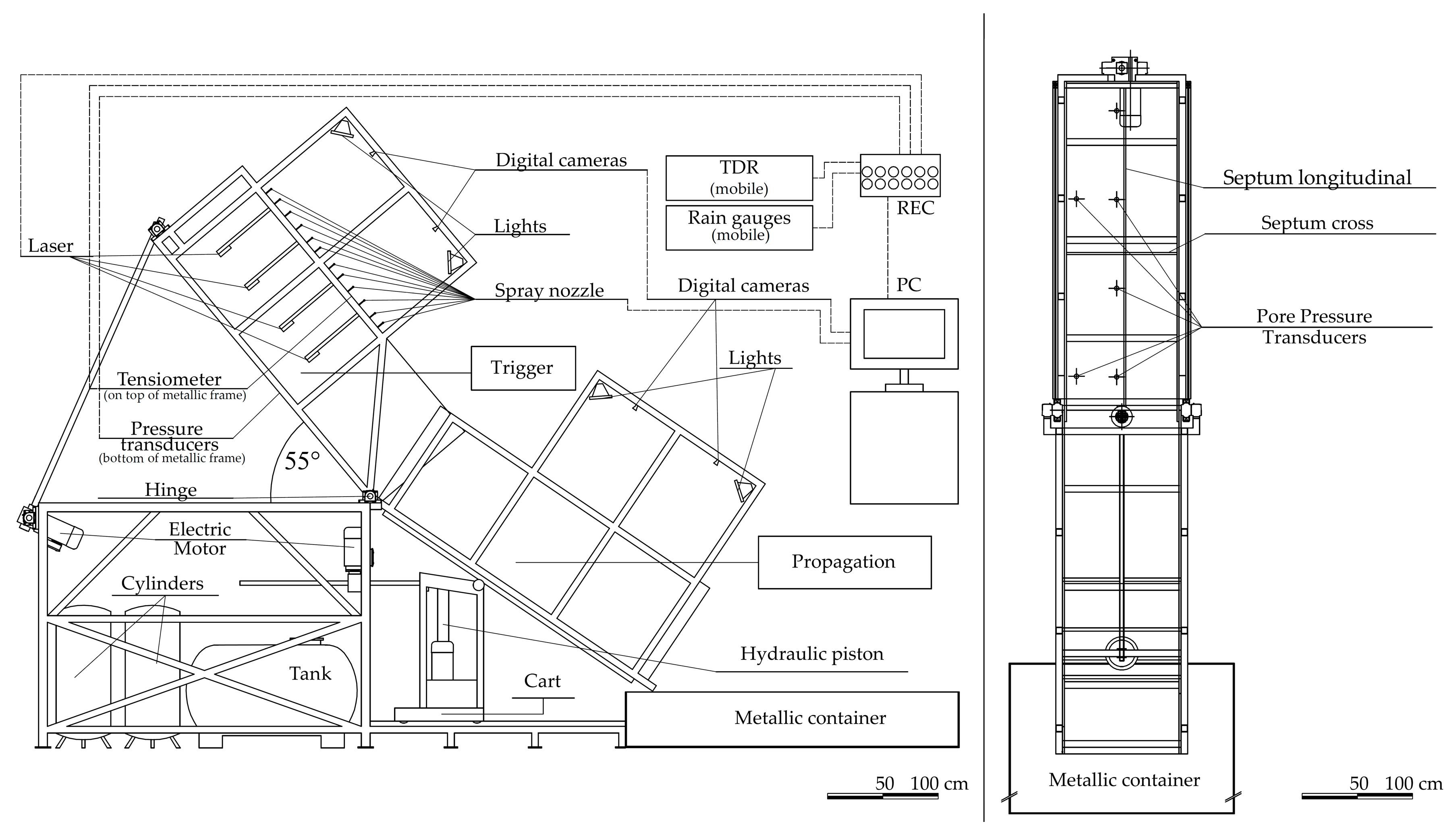
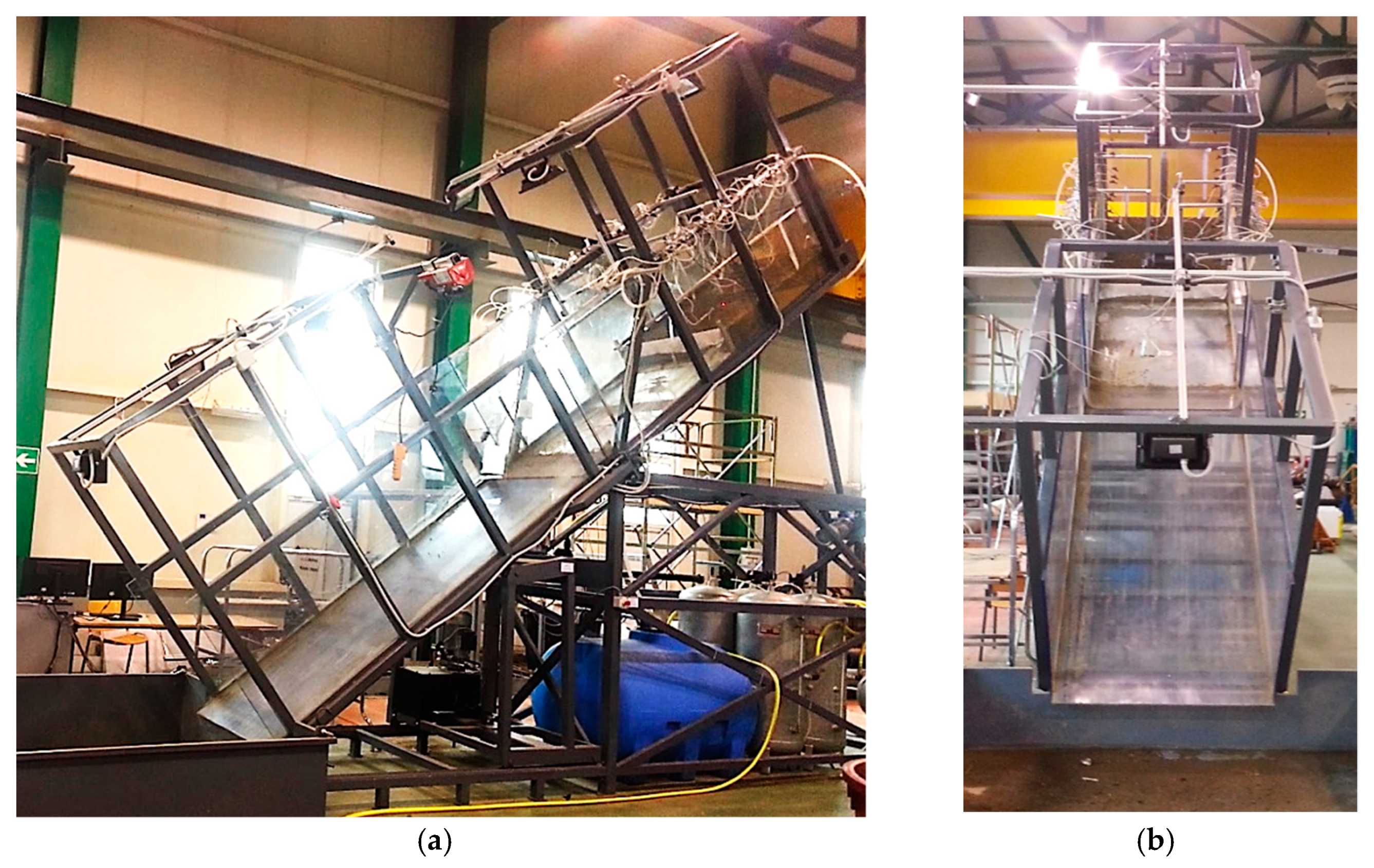
The channel has a rectangular section, which is homogeneous and constant along its entire length. The structure, supported by metal tubes, is 1 m high; 6 m long overall, divided into 3 m for the trigger and 3 m for propagation; and 1 m in width. The section and plan of the mechanical component of the structure are reported in Figure 1, while Figure 2 shows two photographs of the side and front view of the channel.
In the upper flume, drainage channels are installed, which collect the water dripping from the side walls, and dividing walls may be installed, arranged longitudinally and vertically to the axes. This not only allows small study plots to be constructed but also tests to be carried out in parallel. Both the side walls and the bottom wall are made of transparent plexiglass panels to ensure that movement can be both viewed and filmed during the landslide. On the flume bed, it is possible to reproduce both impermeable and permeable bottom bases. In the former case, an impermeable rough bed is laid, which acts as an interface with the test soil, consisting of a plastic sheet on which gravel grains are glued. In the latter case, a permeable geotextile or geonet is used.
To hold the deposit, a draining grid is laid at the foot of the reconstructed slope. Grids of different heights can be inserted according to the thickness of the reconstructed deposit. The grid is formed by a perforated metal sheet, on which a permeable geotextile is placed which permits drainage. Moreover, on the front part of the grid, transversal to the slope, small water collection channels can be mounted to measure both the surface runoff and the runoff from the individual soil layers.
Artificial rainfall was applied with a 24-nozzle water particle sprinkler system, fed by a main 1000-L tank and four 200-L auxiliary tanks. The rainfall system integrates four pressure sensors and three auxiliary rain gauges. The arrangement of the nozzles was optimized to ensure rainfall uniformity, and minimize surface erosion and interference with the video system.
The pressure range varies between 10 and 700 kPa with an intensity that can vary according to the nozzles used. For each nozzle, the maximum variation ranges from 0.28 to 6.13 mm/h and, multiplied by the 24 nozzles, ranges from 6.7 to 147 mm/h. In addition to the artificial rainfall system, further acquisition systems are installed, which permit data collection with a series of sensors for a total of 48 channels from tensiometers, pressure transducer, laser sensors to detect the soil level, auxiliary sensors (slope and pressure) and rain gauges.
The individual sensors are placed in various positions and each may be positioned to operate on various measurement configurations and simulations.
2.2. Sensor System
The instrumentation in the artificial channel can measure the main parameters that control the physical phenomenon, thanks to the installation of the following equipment:
- Tensiometers (used to measure suction);
- Pressure transducers (used to measure pore water pressure);
- TDR device (used to measure soil water content);
- Rainfall system (used to simulate rainfall);
- Laser sensors (used to measure the soil profile and uz displacements); and
- High-resolution video cameras (used to measure displacements along ux and uy).
Figure 2 shows the sensors listed above their relative position along the structure. This sensor system is essential for measuring and monitoring the main parameters, which control and regulate the phenomenon of landslides triggered by rainfall infiltration.
A more complete scheme of the instrumentation with its main properties is reported in Table 1.
2.2.1. Tensiometers
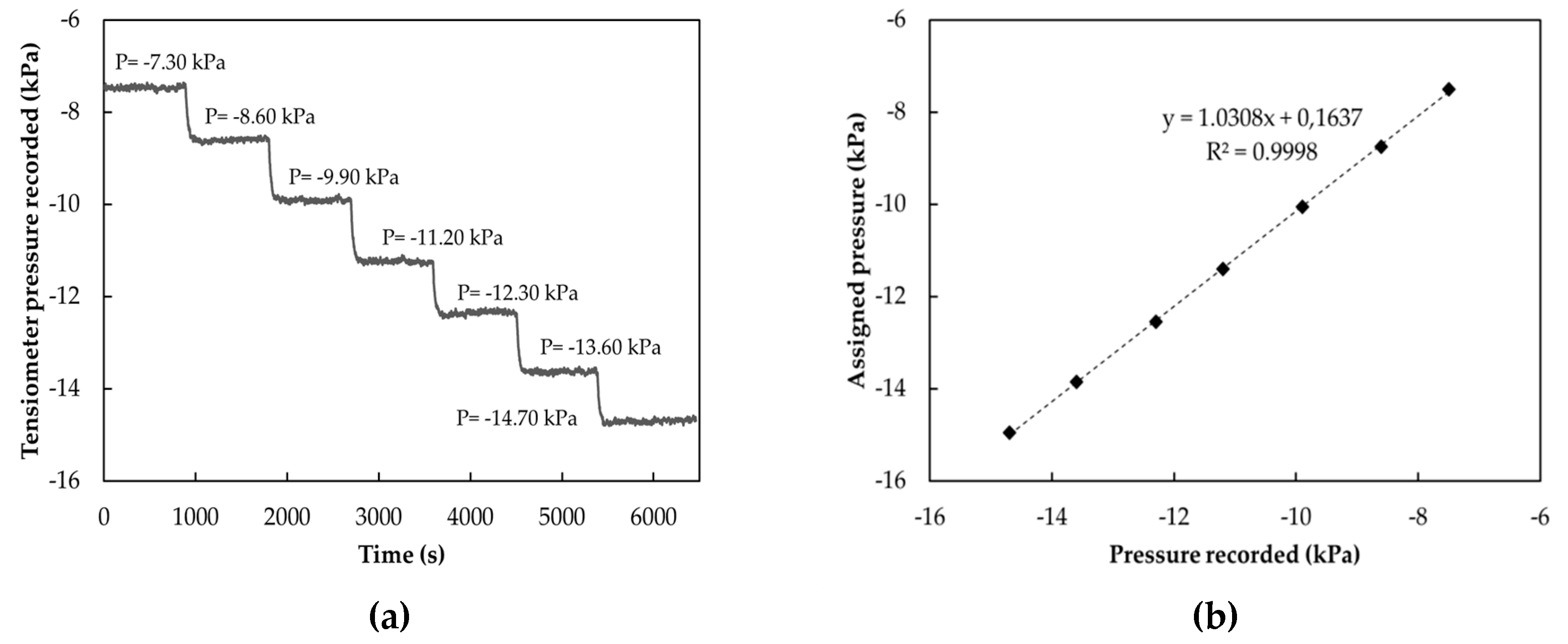
Suction is measured with a series of small-tip tensiometers (model 2100 F—Soilmoisture Equipment Corp.). The body is formed by a transparent plastic rigid tube on which a capsule is lodged for air circuit bleeding as well as an automatic acquisition transducer. The ceramic porous tip, 2.5 cm long and with a diameter of 6 mm, with a nominal air entry value of 100 kPa, is connected to the tensiometric body by means of a capillary tube protected by an external nylon tube 2 m long. The tensiometers are installed in the soil and their functioning is based on the interaction of equilibrium between the porous ceramic cap filled with water and the surrounding soil. These type of tensiometers are unable to measure matrix potentials greater than 100 kPa. Indeed, the range of suction measurement varies between 0 and 100 kPa. To eliminate any instrument errors, each tensiometer should be appropriately calibrated. Calibration consists in comparing pressures recorded by the sensor with different pressures applied. The values recorded by the tensiometer are acquired in various configurations, making the pressure applied vary on each occasion. Thus, different applied pressures are obtained with the relative values recorded and, by including such values in the system, it is possible to construct a regression curve which associates recorded values with actual pressures. An example of calibration of a tensiometer installed on the artificial channel is reported in Figure 3. Figure 3a,b shows, respectively, the pressures recorded by the instrument and the calibration curve obtained with a linear regression.
2.2.2. Pressure Transducers
Neutral pressure transducers are used to measure neutral positive pressures and monitor excess pressures induced by slope failure in the course of tests. The model of transducers installed (LM31-00000F-2 PSIG—TE Connectivity Measurement Specialties), (Hong Kong, China) is a stainless-steel sensor with PVC isolating connector. The transducers are specially lodged on the channel bottom and have to be saturated prior to the soil layer being placed. The membrane is protected by a porous plate, which prevents the inclusion of soil particles. The operative pressure for the series in question is 13.79 kPa (2PSI) with the maximum pressure of 137.9 (20PSI). Precision is ±0.3%, the total error range is ±3%, and the working temperature range is from −20 to 70 °C. The pressure transducers must also be calibrated. The procedure is straightforward and consists in applying above the load cell a water column of known height and recording the output signal from the sensor once it has stabilized. An example of calibration of a pressure transducer installed on an artificial channel is reported in the Figure 4. Figure 4a,b shows, respectively, the pressure values recorded by the instrument and the calibration curve obtained with linear regression.
2.2.3. TDR Device
Time domain reflectometry (TDR) is one of the most widely used techniques to measure soil water content and electrical conductivity both for laboratory tests and for field measurements [19,20,21]. It can be used to determine volumetric water content (θ) indirectly, insofar as the probes do not measure explicitly the quantity of water found in the soil, but determine its relative dielectric constant (εr). The technique is based on measuring the time taken by an electromagnetic wave to cross a metal probe immersed in the soil. The wave propagation velocity (Vp) depends on the soil dielectric permettivity, which in turn depends on the quantity of water present in the sample.
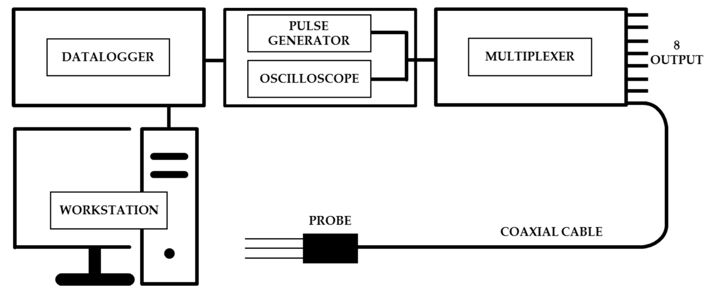
Therefore, relations are needed that couple soil relative dielectric constant with the soil water. There are several calibration relationships, based both on an empirical approach [22,23], and on analytical approach [24]. However, some types of soil (especially with a high percentage of organic material, clay or pyroclastic soil) do not follow these relationships and therefore it is appropriate to define specific calibration curves. The measurement system is illustrated in Figure 5 and comprises a datalogger connected to a system consisting of a generator of rectangular pulses and an oscilloscope connected to a multiplexer, to which eight probes can be connected.
The instrument on the channel consists of a TDR100-based Campbell Scientific System (Logan, UT, USA) connected to various types of probes of different sizes. Moreover, “home-made” TDR probes were also constructed with the same shape as those already installed, but with a preference for smaller size. Smaller probes allow better point-based water content measurements to be obtained and the soil is less disturbed. All the types of probes are produced with three metal rods, i.e., the optimal number, insofar as, by adopting more rods, there is little improvement in results [25].
2.2.4. Laser Displacement Transducer
The artificial channel, in order to monitor the displacements along the orthogonal profile, is equipped with triangulation laser sensors, model LCL45/100 U-485 BI5M—fae (Francisco, CA, USA) This measurement system is based on a simple geometric relation. The distance is determined with extreme precision, using simple trigonometric calculations with a lower resolution at fractions of a micrometer.
Laser point sensors are frequently used due to their simple operation and the ease of alignment with the target thanks to the visible laser spot target. For the model installed, precision and resolution are also obtained in rapid measurements, due to the number of sensors installed (n = 6) and the good arrangement in the channel. The measurement base is 45 mm with a working range of 100 mm and a resolution error of 0.03%, as indicated in the technical data sheet accompanying the instrument.
2.2.5. Image Acquisition System and PIV Technique
Besides monitoring the displacements perpendicular to the surface of the deposit, it is also possible to know longitudinal changes, thanks to an image acquisition system with the relative dedicated particle image velocimetry (PIV) system. For image acquisition, high-resolution (1296 × 966) video cameras (ICX445–Basler) (Ahrensburg, Germany) are used, with two positioned in the triggering zone, two in the propagation zone and two at the side of the channel, thanks to jutting metal supports. Two lenses (Basler, Ahrensburg, Germany) are used with the video cameras (C-Mount High Res - 1/2” - 4 mm - F/1.4 w/lock and Mega - Pixel Lens Fixed FL 8 mm - 2/3” - f/1.1 - f/16), as well as a 10-m digital cable.
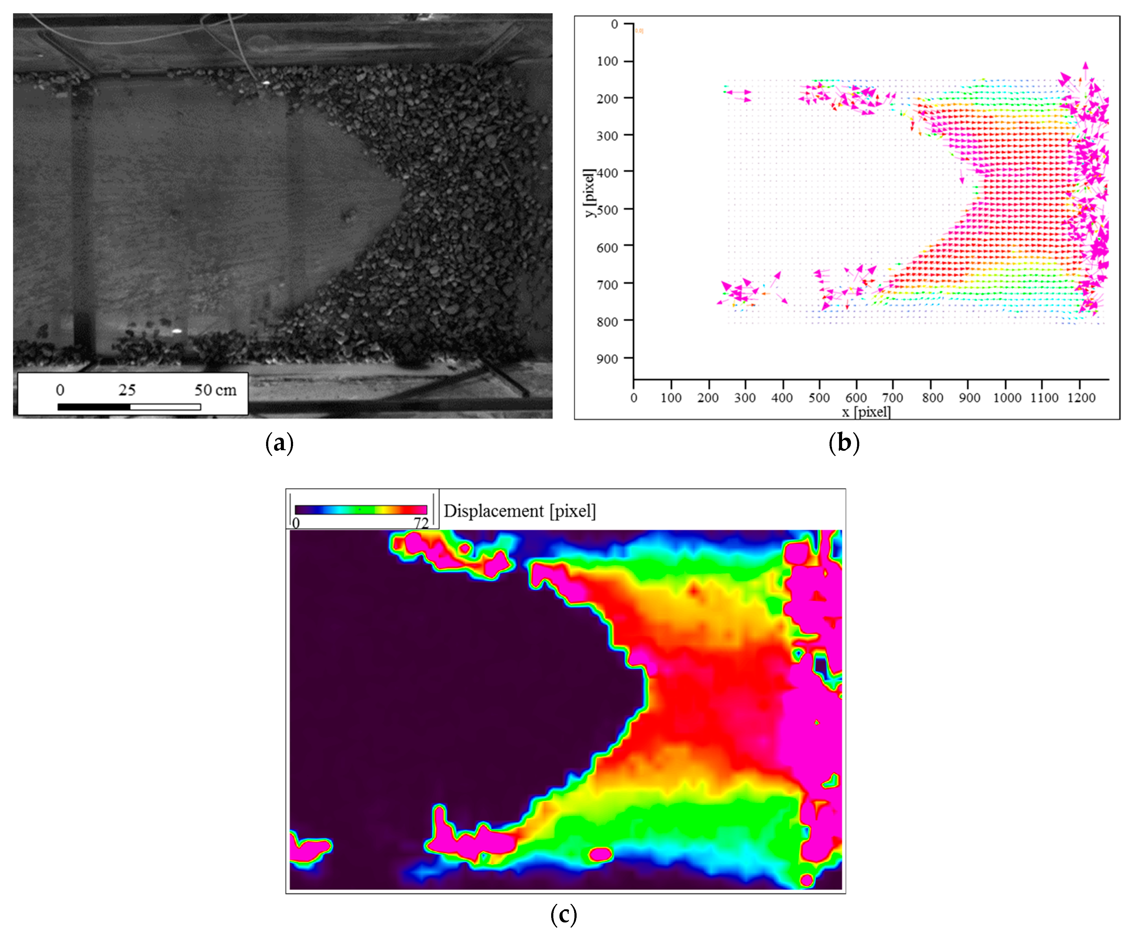
The dedicated PIV system permits optical evaluation of the flow domain of the deposit during the various test phases. It supplies, in a certain section, the projection of the field of instantaneous velocity. From the comparison of the two successive images, the velocity of the space-time relation is evaluated, in other words the pixels between the position of the same particle in two successive photos, and the acquisition time of the two photos. The two images undergo correlation processes, whereby the movements of particles present in each area are compared (32 × 32 or 64 × 64 pixel measurement grid). The density of particles (>25 per window) ensures that correlation processes and average are satisfied. Using PIV acquisition software, the images captured can be processed, correlating and validating the flow domain. To obtain values that are compatible with the real phenomenon, the choice of photogram acquisition frequency is decisive: the interval between two shots must capture the particles in the two consecutive images. The value of Δt will have to oscillate about ∼10 µs. Hence, the technique, through high-resolution image acquisition, allows us to recognize individual soil particles and detect the development of processes generated during the simulation. An example with the results of a simulation on the flume, using PIVview2C software, is reported in Figure 6. The first images concern the field of velocity, with the next showing images at saturation, which present the displacement patterns.
2.2.6. Rainfall System
The system integrates a 24-nozzle rainfall simulator, the main 1000-L tank and four 200-L auxiliary tanks. The system has four pressure sensors and five rain gauges.
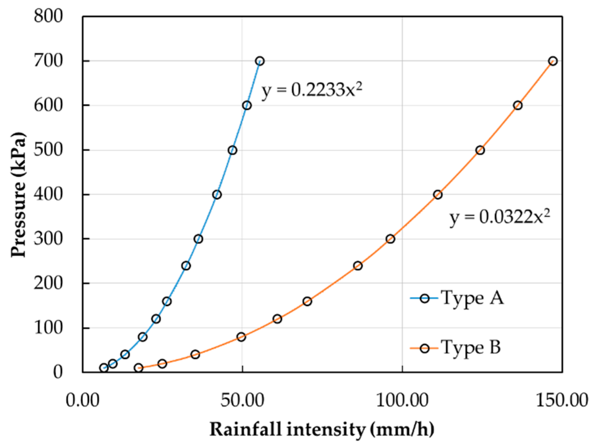
Flows are monitored by pressure sensors and flow regulation is based on the control of pressure from a compressor and a tank outside the system. The nozzles may be one of two types (Type A with less flow or Type B with greater flow), with different flows in relation to the different pressure. Figure 7 illustrates the relationship between flow and pressure; to regulate the flow in a broader range, duty cycle control is possible (partial activation in time) and/or total closure of some nozzles through taps situated at the various distributors. To regulate supply, four groups of each are connected to a collector equipped with a pressure sensor. It is thus possible to regulate the supply pressure from six nozzles independently to optimize flows at four different heights. The rainfall intensity used varies according to the physical model adopted and the reference hyetograph.
2.2.7. Rainfall System
Rain gauges are used to measure and verify rainfall. To date, the system uses five rain gauges (model PCR800—Oregon Scientific) connected to an acquisition system, which allows data to be recorded and automatically saved. The rain gauge consists of a collection funnel and a tipping bucket connected to a magnet, which activates a relay that, in turn, generates a pulse recorder by a counter. Each bucket is equivalent to 1.3 mm of rain. When necessary, these instruments may be easily used to measure flows which are generated within the system. Indeed, if placed downstream of the system of collection channels, using tubes arranged to channel the water leaving the layers, they restore the surface and sub-surface flows.
3. Using Device
A test performed with the device is reported below. In particular, a test was carried out reconstructing a volcanic ash homogeneous deposit. The test was divided into different phases of infiltration and evaporation.
3.1. Homogeneous Soil Test
Pyroclastic soil used for experimental tests was collected in Sarno area, South Italy, about 15 km from the volcano Vesuvius. In May 1998, in this area, numerous and rapid mud-flows devastated the Sarno town, causing an enormous number of victims. In these places, the stratigraphy is composed of limestones covered by layers of pyroclastic deposits. These soils are the product of different eruptions of several volcanoes such as Somma-Vesuvius, Flegrei fields and other volcanoes present in the region no longer active. The ashes, coming out after the eruption and carried by the wind, travel for kilometers from the eruption zone, providing a non-uniform stratigraphy for the entire area [26]. Generally, they are incoherent deposits with variable granulometry that range from sands, silty sands and silts (ashes) to sands with gravel (pumice) and gravels. A homogeneous deposit of pyroclastic ash was reconstructed inside the flume test, and this soil is attributable to the Plinian eruption of “Pollena” of 472 B.C. For this soil, before starting the flume test, laboratory tests were made to know the physical properties such as grain size and specific grains weight.
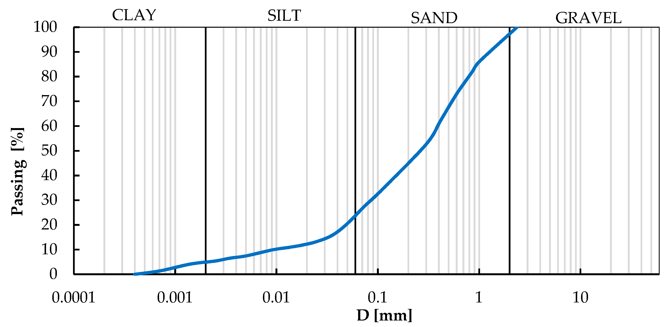
From the grain size distribution (Figure 8), for this soil, the passing percentage for relatively small diameters was evaluated. In fact, the complete evaluation of the curve with a survey by sieving and by sedimentation was carried out. Specific grains weight (γs) was evaluated with the conventional gravimetric method. From the analysis of three tests on soil, a value equal to 2.54 g/cm3 was obtained.
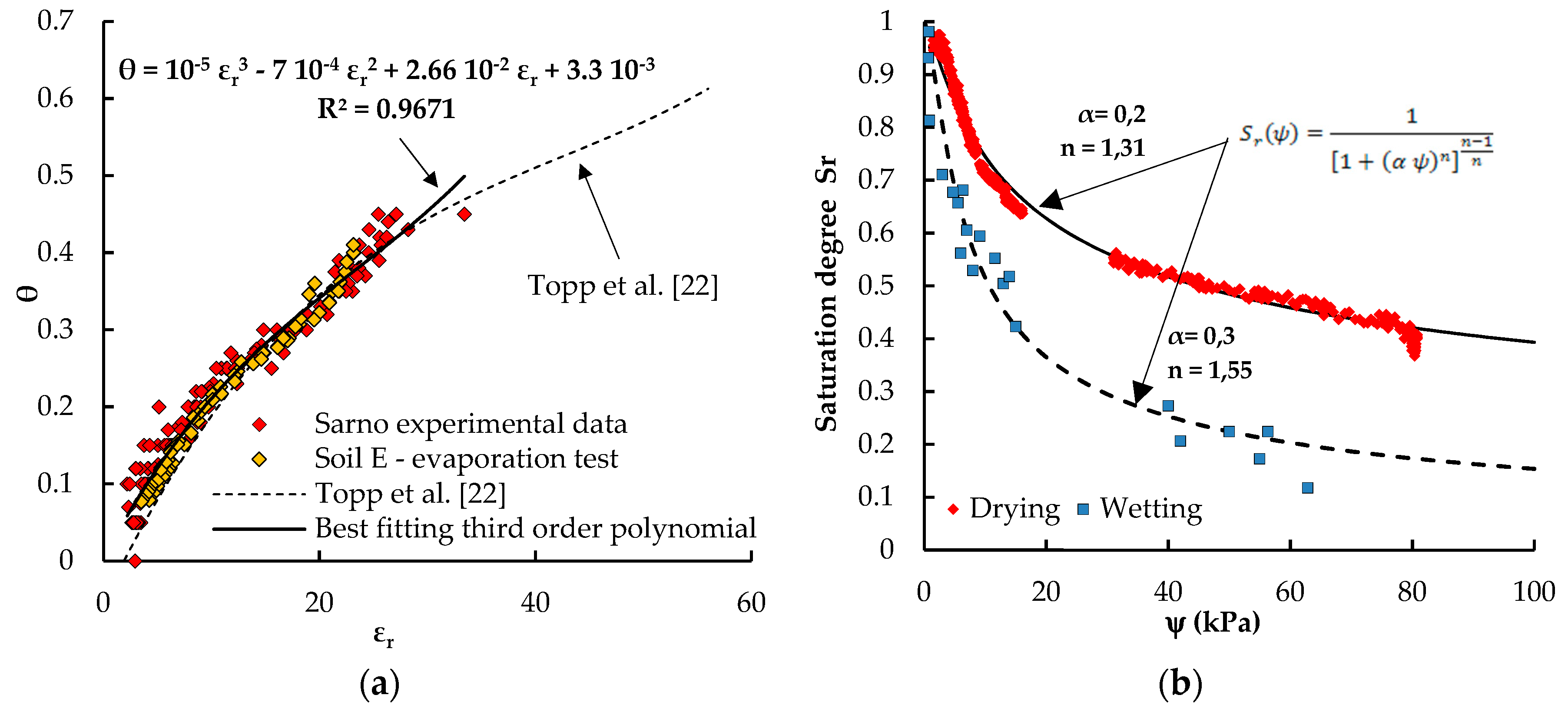
Additional tests were performed to evaluate the dielectric characteristics of the soils and soil water retention curves. This is essential for detecting realistic measurements of water content by using TDR systems and for knowing about the specific hydraulic behavior of the unsaturated soils. Figure 9a,b shows, respectively, an experimental calibration curve that couples volumetric water content (θ) and relative dielectric constant (εr) and soil water retention curves for wetting and dying path.
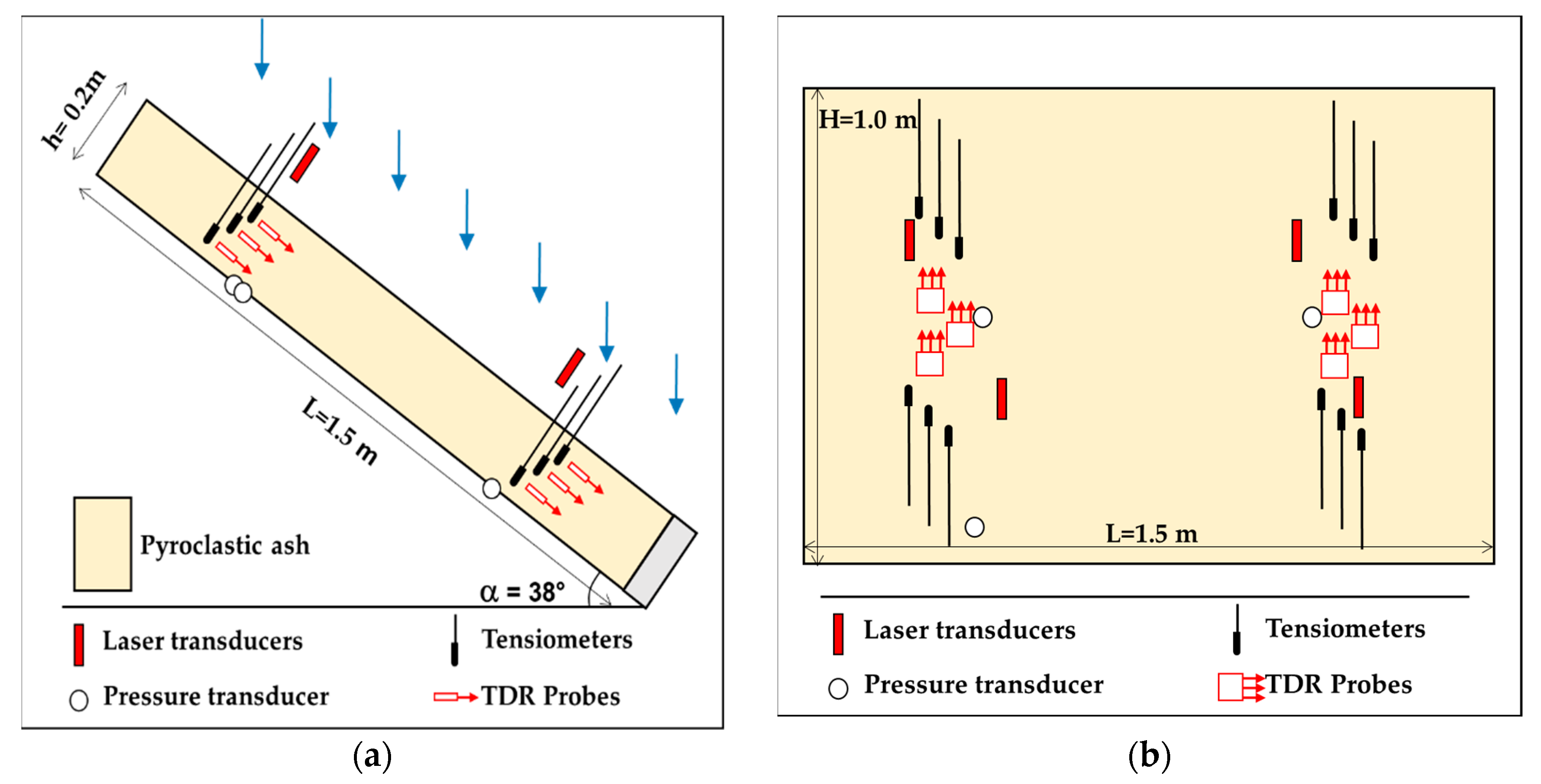
A homogeneous deposit was reconstructed inside the flume. The slope was formed by a layer of volcanic ash 20 cm thick, occupying the entire width of the flume (100 cm) and half length (150 cm). This geometry allowed the deposit to be assimilated to an indefinite slope. At the base of the model, there was an impervious rough bed to simulate conditions similar to those of a natural slope. At the foot of the slope, a geotextile-coated drainage grid was placed. The ash in question was sieved with a 0.4 cm mesh to eliminate coarse material contamination occurring during sampling phase (pumices collapsed inside excavation, vegetable material, etc.). The artificial slope was re-constituted inside the flume by layers, with the moist-tamping technique, with volcanic ash porosity of between 68% and 76% (these values were obtained because, during slope reconstruction, soil weight was measured, with known water content, necessary to occupy the volume), typical in situ conditions. The initial volumetric water content of the ash (θ) was about 20%. Inside the artificial slope, 12 tensiometers were installed to measure suction, and six TDR probes to measure volumetric water content. The sensors were installed at depths of 5 cm, 11 cm and 17 cm below ground surface, in both the upslope and downslope zones of the deposit. On the flume bed, three neutral pressure transducers were arranged, while four laser displacement transducers were installed to measure displacements perpendicular to the slope surface. Figure 10 and Table 2 show schematically the location of the sensors installed inside the deposit.
Rainfall was generated with a sprinkler system placed about 100 cm above the sliding surface.
The nozzles were arranged to ensure rainfall uniformity and avoid surface erosion. Various tests were carried out:
- The first was conducted with the deposit in a horizontal position. Constant rainfall of considerable intensity was simulated (about 220 mm/h) which continued for about 50 min. The test was performed to activate infiltration phenomena to stabilize the slope before tilting it.
- The deposit was then left under natural evaporation for about 14 days, acquiring the values recorded by the various sensors.
- The slope was then inclined at 38°, leaving it in evaporation for about eight days, to redistribute the suction values and water content in the new configuration.
- Finally, a new infiltration phase was simulated, with constant rainfall at an intensity of about 220 mm/h, which lasted until slope failure (about 40 min).
The main characteristics of the various test phases are summarized in Table 3.
3.2. Test Results
During the various tests, values of suction and volumetric water content were acquired in both the upslope and downslope zones at different depths. Displacements perpendicular to the slope surface were also measured, produced by the variation in the tension state, and the water pressure on the flume bed. Acquisition frequency varied according to the type of test. During the phases which envisaged the simulation of rainfall and the relative infiltration of water into the soil, since the monitored values varied rapidly, the acquisition frequency was in the order of seconds. By contrast, during the evaporation phases, the variations were decidedly slower. Hence, it was resolved to acquire values with hourly intervals. The main results of the various test phases are reported below.
3.2.1. Infiltration Phase in a Horizontal Deposit
With the deposit in a horizontal position, rainfall of considerable intensity was simulated (about 220 mm/h). During this phase, all major dimensions were monitored. Figure 11a reports the pattern of matric suction. As can be observed from the graph, the suction values recorded prior to rainfall were very heterogeneous. This great dishomogeneity of values may well have been due to the non-perfect adherence of the porous plates of the tensiometers to the soil. During the sensor installation phase, the porous plates and the tubes connected to them were inserted inside appropriately arranged holes. After installation, the holes were filled, although there was no certainty of the soil adhering to the plates. Any voids that were created close to the porous plates were subsequently filled due to the effect of infiltration processes that were generated after the simulated rainfall. Figure 11a shows that all suction values after rainfall, following a settlement phase, converged on the same values. The TDR measurements were processed by using a calibration equation specifically obtained in this test for volcanic ash. Figure 11b reports the pattern of volumetric soil water content, detected through six TDR probes, while Figure 11c shows the pattern of neutral pressures recorded by pressure transducers on the flume bed. As may be inferred from the results in Figure 11b, the initial volumetric water content, recorded at various depths, appears substantially homogeneous. Deposit configuration ensured that the wetting front advanced vertically homogeneously. Both the neutral pressure transducers placed on the flume bed and most of the tensiometers showed that almost the whole deposit reached conditions of complete saturation. Values of volumetric water content show that at the end of the test the porosity of the deposit was about 60%, indicating a rather compacted condition for the type of soil in question (Note: in the field, porosities of around 75% are frequently observed [27]). This value should come as no surprise, as very loose pyroclastic soils show, when wetted up to conditions close to saturation, the phenomenon of volumetric collapse: under the sole action of tension states deriving from their own weight, they undergo a considerable reduction in volume [28]. The emergence of this phenomenon during the infiltration phase in the flume is attested in Figure 11d, which reports the pattern of displacements experienced by the ground surface top during the test, measured by laser transducers.
As shown in Figure 11d, the soil surface is lowered by several centimeters. The displacement interval ranged from about 2 mm recorded by laser L1 to little more than 1 cm recorded by laser L4. Given the initial thickness of the deposit of about 20 cm, this lowering corresponds to a decrease in porosity, compared with the initial value, of several percentage points (up to around 5% at transducers L1 and L4).
3.2.2. Evaporation Phase in the Horizontal Deposit
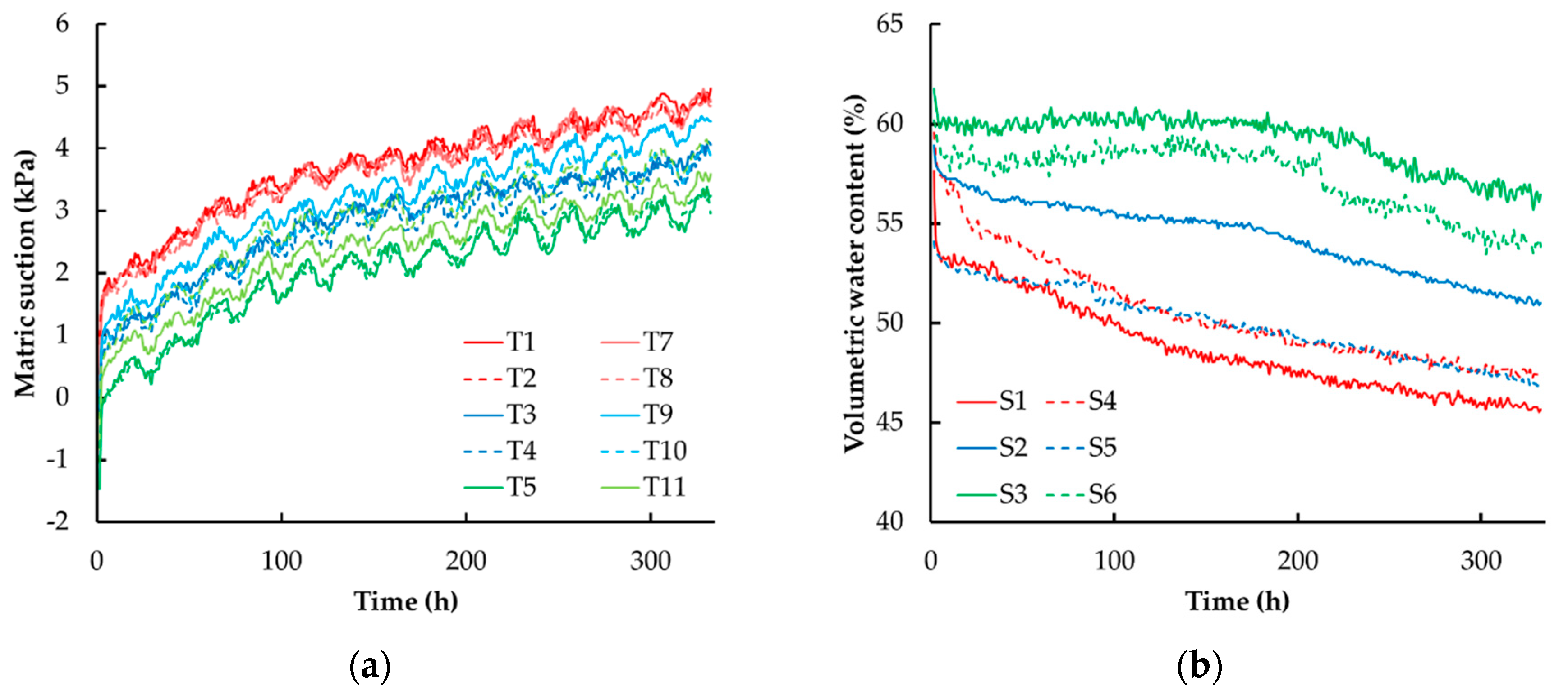
At the end of the infiltration phase, the deposit was left in natural evaporation. This phase lasted about two weeks because the environmental conditions inside the laboratory (relative air humidity about 70% and temperature about 20 °C) produced a very slow evaporative process. Figure 12a shows the pattern of suction recorded by the various tensiometers inside the deposit. It may be inferred from the graph that, after a brief initial phase of rapid suction increase, the phenomenon evolved extremely slowly. The graph also shows the variation in suction obtained in the alternation of day and night. At the end of this phase, suction values between 2 kPa (recorded by the deeper probes) and 5 kPa (recorded by probes closer to the surface) were detected. The trend in volumetric water content recorded by TDR during the evaporation phase is shown in Figure 12b. After a brief initial phase of rapid decrease in water content, there emerged a slow evolution of the phenomenon. At the end of the test, volumetric water content values were between 45% and 57%.
The patterns of values supplied by the probes placed lower down showed that the evaporative flow took over a week to significantly affect also the deeper part of the deposit.
3.2.3. Redistribution Phase in a Sloping Deposit
When the suction recorded inside the deposit settled on values between 3 and 5 kPa, representing conditions that would permit the soil to easily withstand application of a significant increase in shear stress, the slope was tilted up to an angle of about 38°. The channel was tilted very slowly and inclination did not produce deposit movements. The action of gravity, following changes in height, triggered a redistribution of suction and volumetric water content.
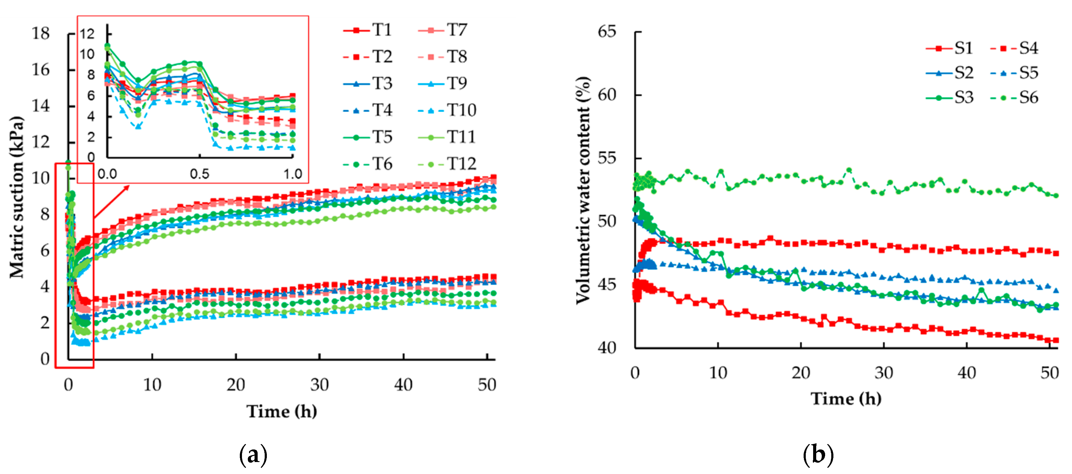
The whole phase lasted about eight days, but as may be noted in Figure 13a, which shows the suction trend in time, there was a significant change already in the first hour. Subsequently, suction values changed slowly, a change produced by evaporation, which became established in the new configuration. The figure also shows that, due to the effect of gravity, the suction values recorded by all the sensors positioned downslope were about 4–5 kPa lower than those upslope (compared to a difference in height of 55 cm).
The variation of depth may also be noted by observing the trend in volumetric water content reported in Figure 13b. In addition, in this case, after a brief transitory phase of redistribution of the volumetric water content, the values changed slowly, a variation produced by evaporation, which was established in the new configuration.
3.2.4. Infiltration Phase in an Inclined Deposit
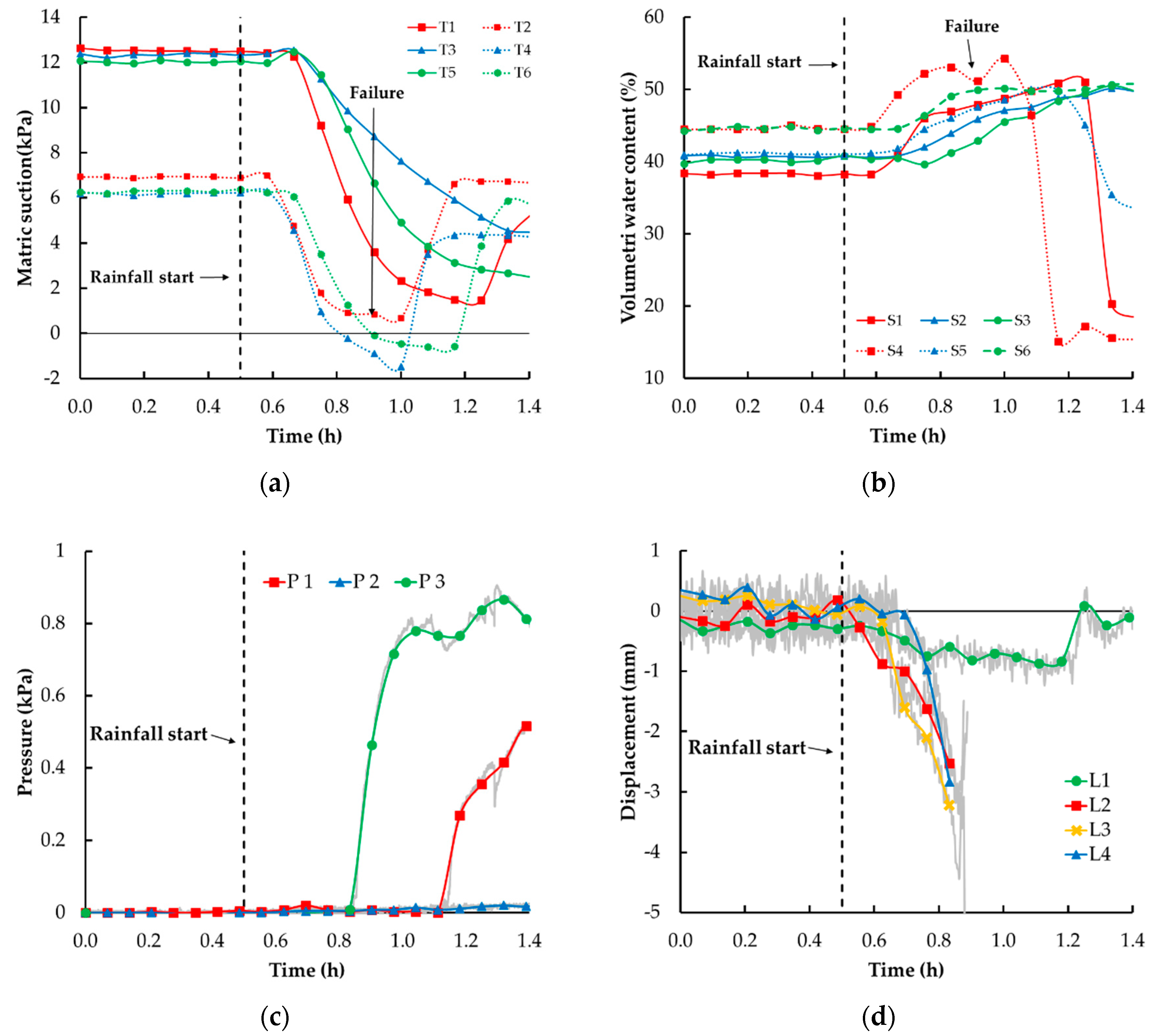
Having determined that the redistribution linked to the change in geometric configuration had been concluded, a further infiltration phase was initiated, with high-intensity artificial rainfall (about 220 mm/h) to reach conditions that would trigger a landslide along the artificial slope. The suction pattern during the last infiltration phase (Figure 14a) clearly shows that saturation conditions at many of the 12 tensiometers were swiftly reached (the figure, to make it more legible, reports only the values of the tensiometers installed on the right-hand side; values recorded by those installed on the left showed the same trend).
Due to gravity filtration processes, at the beginning, suctions near to the downslope section were lower than upslope values. It is also possible to note the moment in which the curves for tensiometers placed downslope at 5 cm and 11 cm of depth had a rapid variation in slope, i.e. when a part of the slope detached and a small surface landslide was triggered.
Trends in soil volumetric water content are reported in Figure 14b, measured with the six TDR probes. In this phase of infiltration in the sloping channel, the progressive advancement of a wetting front from the top was evident, although some differences were observed between the upslope and downslope zones where, due to the sub-surface flow parallel to the slope, the increase in water content was anticipated.
It should also be pointed out that all TDR probes, despite there being absolute evidence that much of the deposit reached complete saturation conditions, detected water content values between 50% and 55%. This is doubtless to be attributed to compaction experienced by the deposit during the previous test phases, which led to a reduction in width from the initial 20 cm to around 18 cm, corresponding to an estimated reduction in porosity of around 10%.
This graph also shows the moment in which a small landslide (2–3 cm deep, between 30 and 50 cm wide and long, positioned in downstream area) detached, producing an abrupt change in the steepness of the curve for the TDR positioned in the most superficial part downslope. In this case, the landslide brought the TDR to the surface and from that point onward the values measured by the sensor were not representative of real water content. The time course of water pressure recorded by the pressure transducers on the flume bed is shown in Figure 14c, while Figure 14d illustrates the trend in displacements perpendicular to the slope surface as recorded by laser displacement transducers. It may be observed (Figure 14c) that the deposit was almost all saturated. Indeed, the transducers (except for P2) recorded an increase in pressure due to the formation of water head on the flume bed, while Figure 14d shows that, during this phase, the slope swelled by a few millimeters.
After a first soils settlement (which occurred at about 0.8–0.9 h), the failure occurs after 1 h with the detachment of a part of the slope and the deactivation of some sensors. After failure, the lasers stopped recording because their measuring range was exceeded (100 mm). L1 was the only laser that provided measurements; it was located in the upstream area where the failure did not affect the slope.
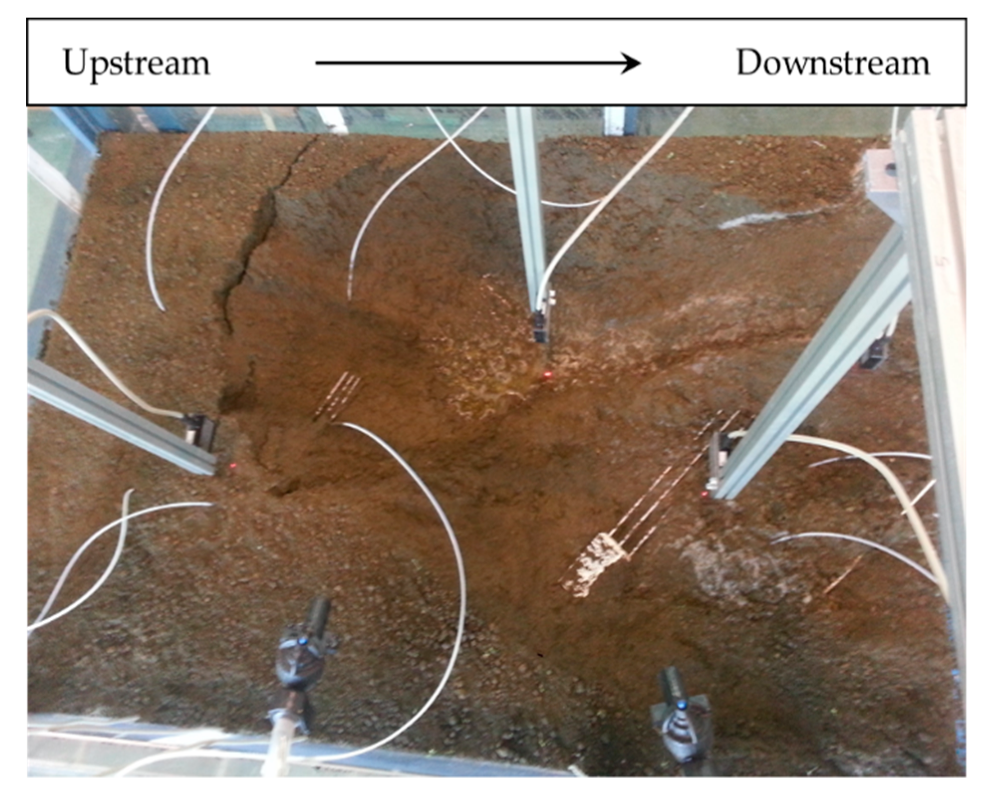
Finally, Figure 15 presents the appearance of the deposit at the end of the test. The figure clearly shows the detachment niche of the landslide and the eroded surface.
3.2.5. General Comment
In general, in the granular soils involved in mud flows, due to its granulometry and the high permeability, failure takes place in essentially drained conditions. Although the process that produces slope failure takes place in drained conditions, many authors have shown that, in the subsequent post-failure phase, an undrained condition can develop, characterized by positive water pressures formation that would produce a reduction in soil strength (static liquefaction [29,30,31]). This hypothesis implies, however, that three conditions occur: the soil is saturated, the transition from a drained to an undrained condition occurs and it is susceptible to liquefy.
Mud flow is possible if soil permeability is sufficiently low. In this way, the positive water pressure remains for a sufficiently long period, during which the landslide develops. Failure can also take place in partial saturation conditions. In this case, a wet front develops, which reduces the suction value and the deposit behaves as a rigid mass [29,32]. If the undrained soil behavior is stable, mud flow does not occur as for the compacted soils. Regarding the test, slope failure, in accordance with the compacted configuration assumed by the deposit during the previous test phases, did not trigger a mud-flow. It showed a progressive erosion of the more superficial soil layers, initially concentrated in the downslope zone, where the intense sub-surface flow resulted in conditions of greater moisture being reached and, at the same time, encouraged soil mobilization. The first local failures began to occur about 20 min after the beginning of rainfall, in areas where suction was less than zero by reducing the effects of apparent cohesion, moving towards the upslope areas.
4. Conclusions
Laboratory tests, which allow observing and measuring phenomena strictly related to landslide mechanisms, are of great importance. For this reason, an instrumented flume, designed and built at the University of Calabria Laboratory of Camilab (Laboratory of Environmental Cartography and Hydraulic and Geological Modelling), has been successfully used to investigate the mechanics of flowslides in cohesionless pyroclastic soils. The use of experimental physical models allows analyzing and observing specific aspects of the landslide mechanism and to measure quantities and physical parameters that affect the failure and post-failure phases.
Thanks to the large size and versatility of use, physical models such as the one proposed in this paper make possible to carry out complex tests, limiting the boundary effects. An example of application wasintroduced on a homogeneous indefinite slope of volcanic ash, through different infiltration and evaporation phases, focusing on water contents and suction levels.
In the test here presented, in addition to the prototype setup, it was possible to develop a first simulation on homogeneous soil from area where mudflow occurred. The test showed that the role of suction and soil density was essential for this type of soil. Failure occurred when the suction was close to zero, reducing the effects of apparent cohesion, while density strongly conditioned the dynamics with which the instability manifested itself. Thickened soil did not allow a mudflow to occur.
Rainfall simulation did not trigger a mud-flow, but it manifested itself as a progressive erosion of the more superficial soil layers. This failure type was due to the compacted configuration assumed by the deposit during the first test phases.
Results need to be deepened and better recognized in the evolution of the water content profile and any significant changes in the displacement field in unsaturated soil slopes subjected to continuous rainfall. Additional tests could clarify the physical process leading to slope failure and provide great help for the rapid assessment of flowslide development. Preliminary experimental results look promising in this respect. Furthermore, it will be necessary to carry out new tests with different soil densities and with stratified soils to complete the landslide evolution scenarios.
Author Contributions
Data curation, G.S. and G.C.; Formal analysis, G.S. and G.C.; Funding acquisition, P.V.; Methodology, G.S. and G.C.; Project administration, P.V.; Software, G.S.; Supervision, G.C. and P.V.; Validation, G.S. and G.C.; Writing—original draft, G.S.; Writing—review & editing, G.C.
Funding
The authors gratefully acknowledge the financial support provided by the framework of the SILA—PONa3_00341 project An Integrated System of Laboratories for the Environment.
Acknowledgments
For design and validation of the physical model, we are indebted to the collaboration of Emilia Damiano, Roberto Greco and Lucio Olivares at the Università degli Studi della Campania Luigi Vanvitelli.
Conflicts of Interest
The authors declare no conflict of interest.
References
- Van Westen, C.J.; van Asch, T.W.J.; Soeters, R. Landslide hazard and risk zonation—Why is it still so difficult? Bull. Eng. Geol. Environ. 2006, 65, 167–184. [Google Scholar] [CrossRef]
- EWCII; ONU; ISDR. Europe, Regional Consultation in Preparation for the Second International Conference on Early Warning (EWCII); Plate, E.J., Ed.; ISDR-International Strategy for Disaster Reduction: Bonn, Germany, 2003. [Google Scholar]
- Vranken, L.; Vantilt, G.; van Den Eeckhaut, M.; Poesen, J. Landslide risk assessment in a densely populated hilly area. Landslides 2015, 12, 787. [Google Scholar] [CrossRef]
- Costanzo, S.; Massa, G.D.; Costanzo, A.; Morrone, L.; Raffo, A.; Spadafora, F.; Borgia, A.; Formetta, G.; Capparelli, G.; Versace, P. Low-cost radars integrated into a landslide early warning system. Adv. Intell. Syst. Comput. 2015, 354, 11–19. [Google Scholar] [CrossRef]
- Alcántara-Ayala, I.; Garnica-Peña, R.J.; Murillo-García, F.G.; Miguel Octavio, S.-O.; Arturo, M.-M.; Atlántida, C.-H. Landslide disaster risk awareness in Mexico: Community access to mapping at local scale. Landslides 2018. [Google Scholar] [CrossRef]
- Sirangelo, B.; Versace, P.; Capparelli, G. Forewarning model for landslides triggered by rainfall based on the analysis of historical data file. IAHS-AISH Publ. 2003, 278, 298–304. [Google Scholar]
- Iverson, R. Landslide triggering by rain infiltration. Water Resour. Res. 2000, 36, 1897–1910. [Google Scholar] [CrossRef] [Green Version]
- Godt, J.W.; Sener-Kaya, B.; Lu, N.; Baum, R.L. Stability of infinite slopes under transient partially saturated seepage conditions. Water Resour. Res. 2012, 48, 1–14. [Google Scholar] [CrossRef]
- Capparelli, G.; Versace, P. FLaIR and SUSHI: Two mathematical models for Early Warning Systems for rainfall induced landslides. Landslides 2011, 8, 67–79. [Google Scholar] [CrossRef]
- Arnone, E.; Noto, L.V.; Lepore, C.; Bras, R.L. Physically-based and distributed approach to analyze rainfall-triggered landslides at watershed scale. Geomorphology 2011, 133, 121–131. [Google Scholar] [CrossRef]
- Formetta, G.; Capparelli, G.; Versace, P. Evaluating performance of simplified physically based models for shallow landslide susceptibility. Hydrol. Earth Syst. Sci. 2016, 20, 4585–4603. [Google Scholar] [CrossRef] [Green Version]
- Iverson, R.M.; LaHusen, R.G. Dynamic pore pressure fluctuations in rapidly shearing granular materials. Science 1989, 246, 796–799. [Google Scholar] [CrossRef] [PubMed]
- Eckersley, J.D. Instrumented laboratory flowslides. Géotechnique 1990, 40, 489–502. [Google Scholar] [CrossRef]
- Spence, K.J.; Guymer, I. Small-scale laboratory flowslides. Géotechnique 1997, 47, 915–932. [Google Scholar] [CrossRef]
- Wang, G.; Sassa, K. Factors affecting rainfall-induced landslides in laboratory flume tests. Géotechnique 2001, 51, 587–599. [Google Scholar] [CrossRef]
- Okura, Y.; Ochiai, H.; Sammori, T. Flow failure caused by monotonic liquefaction. In Proceedings of the International Symposium: Landslide Risk Mitigation and Protection of Cultural and Natural Heritage, Kyoto, Japan, 21–25 January 2002; pp. 155–172. [Google Scholar]
- Lacerda, W.A.; Avelar, A.S. Flume tests on sand subjected to seepage with the influence of hidden barriers. In Proceedings of the International Workshop on Occurrence and Mechanisms of Flows in Natural Slopes and Earthfills, Sorrento, Italy, 14–16 May 2003. [Google Scholar]
- Olivares, L.; Damiano, E.; Greco, R.; Zeni, L.; Picarelli, L.; Minardo, A.; Guida, A.; Bernini, R. An Instrumented Flume to Investigate the Mechanics of Rainfall-Induced Landslides in Unsaturated Granular Soils. Geotech. Test. J. 2009, 32. [Google Scholar] [CrossRef]
- Dasberg, S.; Dalton, F.N. Time domain reflectometry field measurement of soil water content and electrical conductivity. Soil Sci. Soc. Am. J. 1985, 49, 293–297. [Google Scholar] [CrossRef]
- German, P.F.; Di Pietro, L.; Singh, V.P. Momentum of flow in soils assessed with TDR moisture readings. Geoderma 1997, 80, 153–168. [Google Scholar] [CrossRef]
- Greco, R. Soil water content inverse profiling from single TDR waveforms. J. Hydrol. 2006, 17, 325–339. [Google Scholar] [CrossRef]
- Topp, G.C.; Davis, J.L.; Annan, A.P. Electromagnetic determination of soil water content: Measurement in coaxial transmission lines. Water Resour. Res. 1980, 16, 574–582. [Google Scholar] [CrossRef]
- Regalado, C.M.; Munoz Carena, R.; Socorro, A.R.; Hernandez Moreno, J.M. Time domain reflectometry models as a tool to understand the dielectric response of volcanic soils. Geoderma 2003, 117, 313–330. [Google Scholar] [CrossRef]
- Roth, K.; Schulin, R.; Flühler, H.; Attinger, W. Calibration of Tim Domain Reflectometry for Water Content Measurement Using a Composite Dieletric Approach. Water Resour. Res. 1990, 26, 2267–2273. [Google Scholar] [CrossRef]
- Zegelin, S.J.; White, I.; Russel, G.F. A Critique of the Time Domain Reflectometry Technique for Determining Field Soil-Water Content. Advances in Measurement of Soil Physical Properties: Bringing Theory into Practice. Soil Sci. Soc. Am. J. 1992, 30, 187–208. [Google Scholar] [CrossRef]
- Del Prete, M.; Guadagno, F.M.; Hawkins, A.B. Preliminary report on the landslides of 5 May 1998, Campania, southern Italy. Bull. Eng. Geol. Environ. 1998, 57, 113–129. [Google Scholar] [CrossRef]
- Bilotta, E.; Cascini, L.; Foresta, V.; Sorbino, G. Geotechnical characterisation of pyroclastic soils involved in huge flowslides. Geotech. Geol. Eng. 2005, 23, 365–402. [Google Scholar] [CrossRef]
- Cascini, L.; Cuomo, S.; Pastor, M.; Sorbino, G. Modeling of rainfall-induced shallow landslides of the flow-type. J. Geotech. Geoenviron. Eng. 2010, 136, 85–98. [Google Scholar] [CrossRef]
- Collins, B.D.; Znidarcic, D. Stability analyses of rainfall induced landslides. J. Geotech. Geoenviron. 2004, 130, 362–371. [Google Scholar] [CrossRef]
- Take, W.A.; Bolton, M.D.; Wong, P.C.P.; Yeung, F.J. Evaluation of landslide triggering mechanisms in model fill slopes. Landslides 2004, 1, 173–184. [Google Scholar] [CrossRef]
- Sassa, K.; Wang, G.H. Mechanism of landslide-triggered debris flows: Liquefaction phenomena due to the undrained loading of torrent deposits. Debris-flow Hazards Relat. Phenom. 2005, 81–104. [Google Scholar] [CrossRef]
- Rahardjo, H.; Lim, T.T.; Chang, M.F.; Fredlund, D.G. Shear strength characteristics of a residual soil. Can. Geotech. J. 1995, 32, 60–77. [Google Scholar] [CrossRef]
Figure 1.
Section and plan of the mechanical components of flume.

Figure 2.
Physical model: (a) side view; and (b) frontal view.

Figure 3.
Example of calibration of a tensiometer: (a) the graph shows the recorded response, in terms of pressure values, of the instrument at the various pressures applied; and (b) the graph shows the calibration curve of the tensiometer used.
Figure 3.
Example of calibration of a tensiometer: (a) the graph shows the recorded response, in terms of pressure values, of the instrument at the various pressures applied; and (b) the graph shows the calibration curve of the tensiometer used.

Figure 4.
Example of calibration of a pressure transducer:(a) the graph shows the recorded response, in terms of pressure values, of the device at the various pressures applied; and (b) the graph shows the calibration curve of the transducer used.
Figure 4.
Example of calibration of a pressure transducer:(a) the graph shows the recorded response, in terms of pressure values, of the device at the various pressures applied; and (b) the graph shows the calibration curve of the transducer used.

Figure 5.
TDR device.

Figure 6.
(a) Instant of a test; (b) field of velocity; and (c) field of displacements.

Figure 7.
Rainfall intensity vs. pressure.

Figure 8.
Grain size distribution for soil tested. The soil is a silty sand.

Figure 9.
(a) Experimental calibration curve that couples volumetric water content with soil relative dielectric constant; and (b) drying and wetting soil water retention curve, fitted by Van Genuchten equation (hp. θr = 0).
Figure 9.
(a) Experimental calibration curve that couples volumetric water content with soil relative dielectric constant; and (b) drying and wetting soil water retention curve, fitted by Van Genuchten equation (hp. θr = 0).

Figure 10.
(a) Position of the sensors in section; and (b) position of the sensors (plan).

Figure 11.
Parameters graphs monitored during the infiltration phase in the horizontal deposit: (a) suction; (b) volumetric water content; (c) pore water pressure at the bottom of flume; and (d) orthogonal displacements by the soil surface.
Figure 11.
Parameters graphs monitored during the infiltration phase in the horizontal deposit: (a) suction; (b) volumetric water content; (c) pore water pressure at the bottom of flume; and (d) orthogonal displacements by the soil surface.

Figure 12.
Parameters graphs monitored during the evaporation phase in the horizontal deposit: (a) suction; and (b) volumetric water content.
Figure 12.
Parameters graphs monitored during the evaporation phase in the horizontal deposit: (a) suction; and (b) volumetric water content.

Figure 13.
Parameters graphs monitored during the redistribution phase in a sloping deposit: (a) suction; and (b) volumetric water content.
Figure 13.
Parameters graphs monitored during the redistribution phase in a sloping deposit: (a) suction; and (b) volumetric water content.

Figure 14.
Parameters graphs monitored during the infiltration phase in a sloping deposit: (a) suction; (b) volumetric water content; (c) pore water pressure at the bottom of flume; and (d) orthogonal displacements by the soil surface.
Figure 14.
Parameters graphs monitored during the infiltration phase in a sloping deposit: (a) suction; (b) volumetric water content; (c) pore water pressure at the bottom of flume; and (d) orthogonal displacements by the soil surface.

Figure 15.
Deposit at the end of the test.


Table 1.
Main characteristics of devices.
| Measurement | Device | Manufscture/Type | Sensor | Diameter | Height | Transducer | Operating Range | Linearity | Hysteresis | Output | Sampling Rrequency | |
| Matric suction | Tensiometer | Soil Moisture Corp/2100F | Porous ceramic cup | 6 mm | 25 mm | Current transducer | 0–100 Pa | 0.0025 | <1% | 4–20 mA | 750 Hz | |
| Measurement | Device | Manufscture/Type | Sensor | Diameter | Length | Time Response of Combined Pulse Generator & Sampling Circuit | Maximum spatial resolution | Operating Temperature Range | Timing Resolution | |||
| Water content profile along z | TDR apparatus | TDR100 Campbell Scientific | Small probe | 2 mm | 75 mm | ≤300 ps | 1 cm at θ = 0.1 m3/m3 | 2 cm at θ = 0.2 m3/m3 | −40/55 °C | 12.2 ps | ||
| Medium probe | 3 mm | 150 mm | ≤300 ps | 1 cm at θ = 0.1 m3/m3 | 2 cm at θ = 0.2 m3/m3 | −40/55 °C | 12.2 ps | |||||
| Large probe | 5 mm | 300 mm | ≤300 ps | 1 cm at θ = 0.1 m3/m3 | 2 cm at θ = 0.2 m3/m3 | −40/55 °C | 12.2 ps | |||||
| Home-made metallic probe | 2.2 mm | 80 mm | ≤300 ps | 1 cm at θ = 0.1 m3/m3 | 2 cm at θ = 0.2 m3/m3 | −40/55 °C | 12.2 ps | |||||
| Measurement | Device | Manufscture/Type | Sensor | Housing size (L by W by H) | Mesuring range | Resolution | Linearity | Output | Operating Temperature | Sampling frequency | ||
| Vertical Displacements | Sensor displacement | LCL 45/100 - fae | Laser CMOS -array | 62 mm by 17 mm by 50 mm | 100 mm | 0.03% | ± 0.2% | 4–20 Ma (analogic) RS485 kbits/s (Digital) | −10 /60 °C | 2 kHz | ||
| Measurement | Device | Manufscture/Type | Sensor | Housing size (L by W by H) | Frame Rate | Resolution | Pixel size | Video output | Image area | Power Consuption | ||
| Displacements ux - uy | Digital camera | Basler/ICX445 | 1/3" progressive Scan CCD | 42 mm by 29 mm by 29 mm | 22 fps | 1296 by 966 | 3.75 μm by 3.75 μm | YUV 4:2:2 Mono - Bayer | 100 cm by 150 cm | 2.5 W (PoE) 2.2 (AUX) | ||
| Accessory: Lens C-Mount High Res - 1/2” - 4 mm - F/1.4 w/lock Basler Digital I/O cable with HRS 6-pin connector, 10 m Mega–Pixel Lens Fixed FL 8 mm - 2/3” - f/1.1 - f/16 | ||||||||||||
| Measurement | Device | Manufscture/Type | Sensor | Diameter | Height | Operating range | Resolution | Accuracy | Output | Operating Temperature | Compensated Temperature | |
| Pore water pressure | Pore pressure transducer | TE Connectivity Measurement Specialties LM31-00000F-002PG | SENSOR 2PSIG 1/2NPT 0.5-4.5 V 12” Inox and PVC | 12.7 mm | 25.4 mm | 0–3.79 kPa | 0.3% | ± 1% | 0–5 V | −20/70 °C | 0–40°C | |
| Measurement | Device | Manufscture/Type | Sensor | Diameter | Height | Operating range | Resolution | Maximum temporal Resolution | ||||
| Rainfall intensity | Rain gauge | Oregon Scientific PCR800 | Tiping bucket | 87 mm | 107 mm | 0–999 mm/h | 1 mm/h | 1 min | ||||
Table 2.
Sensors position.
| Tensiometers | TDR Probes | ||||
|---|---|---|---|---|---|
| # | Position | Depth | # | Position | Depth |
| T1 | Upstream—right | 5 cm | S1 | Upstream | 5 cm |
| T2 | Downstream—right | 5 cm | S2 | Upstream | 11 cm |
| T3 | Upstream—right | 11 cm | S3 | Upstream | 17 cm |
| T4 | Downstream—right | 11 cm | S4 | Downstream | 5 cm |
| T5 | Upstream—right | 17 cm | S5 | Downstream | 11 cm |
| T6 | Downstream—right | 17 cm | S6 | Downstream | 17 cm |
| T7 | Upstream—left | 5 cm | Laser | ||
| T8 | Downstream—left | 5 cm | # | Distance from upstream wall | |
| T9 | Upstream—left | 11 cm | L1 | 30 cm | |
| T10 | Downstream—left | 11 cm | L2 | 50 cm | |
| T11 | Upstream—left | 17 cm | L3 | 90 cm | |
| T12 | Downstream—left | 17 cm | L4 | 110 cm | |
Table 3.
Main characteristics of the various test phases.
| Test | Pattern | Angle (°) | Rainfall (mm/h) | Testing Time |
|---|---|---|---|---|
| Horizontal deposit infiltration |  | 0 | 220 | 50 min |
| Evaporation |  | 0 | 0 | 14 days |
| Redistribution |  | 38 | 0 | 8 days |
| Failure |  | 38 | 220 | 40 min |
© 2019 by the authors. Licensee MDPI, Basel, Switzerland. This article is an open access article distributed under the terms and conditions of the Creative Commons Attribution (CC BY) license (http://creativecommons.org/licenses/by/4.0/).
Share and Cite
MDPI and ACS Style
Spolverino, G.; Capparelli, G.; Versace, P. An Instrumented Flume for Infiltration Process Modeling, Landslide Triggering and Propagation. Geosciences 2019, 9, 108. https://doi.org/10.3390/geosciences9030108
AMA Style
Spolverino G, Capparelli G, Versace P. An Instrumented Flume for Infiltration Process Modeling, Landslide Triggering and Propagation. Geosciences. 2019; 9(3):108. https://doi.org/10.3390/geosciences9030108
Chicago/Turabian StyleSpolverino, Gennaro, Giovanna Capparelli, and Pasquale Versace. 2019. "An Instrumented Flume for Infiltration Process Modeling, Landslide Triggering and Propagation" Geosciences 9, no. 3: 108. https://doi.org/10.3390/geosciences9030108
Note that from the first issue of 2016, this journal uses article numbers instead of page numbers. See further details here.