Numerical Simulation of Conservation Laws with Moving Grid Nodes: Application to Tsunami Wave Modelling


1
Institute of Computational Technologies of Siberian Branch of the Russian Academy of Sciences, 630090 Novosibirsk, Russia
2
Univ. Grenoble Alpes, Univ. Savoie Mont Blanc, CNRS, LAMA, 73000 Chambéry, France
3
LAMA UMR 5127 CNRS, Université Savoie Mont Blanc, Campus Scientifique, 73376 Le Bourget-du-Lac CEDEX, France
4
School of Mathematics, Statistics and Operations Research, Victoria University of Wellington, P.O. Box 600, Wellington 6140, New Zealand
5
Department of Radiology, Medical Physics, Medical Center, Faculty of Medicine, University of Freiburg, 79106 Freiburg, Germany
*
Author to whom correspondence should be addressed.
Geosciences 2019, 9(5), 197; https://doi.org/10.3390/geosciences9050197
Submission received: 22 March 2019
/
Revised: 18 April 2019
/
Accepted: 24 April 2019
/
Published: 30 April 2019
(This article belongs to the Special Issue Interdisciplinary Geosciences Perspectives of Tsunami Volume 2)
Abstract
:In the present article, we describe a few simple and efficient finite volume type schemes on moving grids in one spatial dimension combined with an appropriate predictor–corrector method to achieve higher resolutions. The underlying finite volume scheme is conservative, and it is accurate up to the second order in space. The main novelty consists in the motion of the grid. This new dynamic aspect can be used to resolve better the areas with large solution gradients or any other special features. No interpolation procedure is employed; thus, unnecessary solution smearing is avoided, and therefore, our method enjoys excellent conservation properties. The resulting grid is completely redistributed according to the choice of the so-called monitor function. Several more or less universal choices of the monitor function are provided. Finally, the performance of the proposed algorithm is illustrated on several examples stemming from the simple linear advection to the simulation of complex shallow water waves. The exact well-balanced property is proven. We believe that the techniques described in our paper can be beneficially used to model tsunami wave propagation and run-up.
Keywords:
conservation laws; finite volumes; conservative finite differences; moving grids; adaptivity; advection; shallow water equations; wave run-upMSC:
74S10 (primary); 74J15; 74J30 (secondary)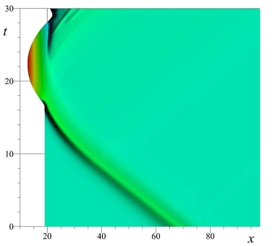
1. Introduction
The main goal of the present manuscript consists in introducing to the tsunami modelling community some state-of-the-art numerical methods for solving nonlinear hyperbolic equations, which allow the use of the available degrees of freedom in the (nearly-) optimal way. Until the last 15 years, tsunami wave modelling has been done in the framework of Nonlinear Shallow Water Equations (NSWE). The numerical simulations have been performed by practitioners essentially with several well-established community codes. To give a few examples, let us mention the code TUNAMI [1] based on a conservative finite difference leap-frog scheme on staggered grids. This scheme approximates NSWE on real bathymetries. Another widely used code is MOST, which is based on the dimensional splitting method (This technique is also known as the alternating directions) [2,3]. We would like to mention also the software COMCOT, which is based on a modified leap-frog scheme discretizing NSWE in Cartesian and spherical coordinates [4]. Finally, in the Institute of Computational Technologies (SB RAS) an in-house software, MGC, based on the finite difference MacCormack scheme in spherical coordinates was developed as well [5].
A big boost in tsunami research happened after Tsunami Boxing day [6] due to the availability of real world data. After this Sumatra 2004 event, several studies questioned the importance of dispersive effects for transoceanic tsunami propagation [7,8,9]. Their conclusions were supported by comparisons of numerical results with field and DART buoy data. We can only mention that the importance of dispersive effects has been already highlighted in 1982 by Mirchina and Pelinovsky [10]:
The considerations and estimates for actual tsunamis indicate that nonlinearity and dispersion can appreciably affect the tsunami wave propagation at large distances.
One of the first tsunami numerical models including spherical effects and linear dispersive terms was TUNAMI-N2. A sensitivity study was performed in Reference [11] on the example of the Sumatra 2004 event. The reported results were in favor of including dispersive effects. Another Weakly Nonlinear Weakly Dispersive (WNWD) model was presented in Reference [12,13]. It was basically a spherical counterpart of the classical Peregrine system [14]. Let us mention also the study by Glimsdal et al. [15] where the importance of dispersion has been investigated numerically and the use of the Fully Nonlinear Weakly Dispersive (FNWD) model was recommended. Such FNWD spherical equations (with the horizontal velocity defined on a certain surface inside the fluid bulk) have been derived in Reference [16]; however, only WNWD numerical results were presented. In a recent work [17], a systematic derivation of spherical rotating FNWD (and WNWD) models have been performed and the so-called base model was derived, which incorporates many other models as particular cases. The reduction of spherical FNWD to WNWD models was illustrated, and several known models were recovered in this way. Finally, the fully nonlinear numerical results have been presented in Reference [18]. In particular, the importance of sphericity, Coriolis, and dispersion effects was thoroughly discussed. The numerical algorithm employed in Reference [18] is based on the splitting approach: An elliptic equation is solved to determine the non-hydrostatic pressure component, and an evolution system of hyperbolic equations with source terms is solved to advance in time the velocity and water height variables. The algorithm was implemented as an explicit two-step predictor–corrector scheme. The volume of publication [18] did not allow the authors to describe all details of the employed numerical method. Henceforth, if we adopt dispersive models for tsunami simulations (It seems now that future generation tsunami modelling codes will include at least some dispersive effects), there is a clear need in robust numerical methods to solve hyperbolic balance equations. The present manuscript should be considered as a tutorial-style article to introduce moving grid algorithms to the developers of future generation tsunami propagation codes.
The numerical simulation of conservation laws is one of the most dynamic and central parts of modern numerical analysis. The systems of conservation laws appear in many fields ranging from traffic modeling [19] to shallow water modelling [20] and compressible fluid mechanics [21]. The finite volume method was proposed in a pioneering work of S. Godunov [22,23] and developed later by Ph. Roe [24] and many other researchers (see Reference [25] for the current state of the art).
Nowadays, the complexity of the problems which arise in practice is such that we have to think about the optimal usage of available computational resources. In this way, the community came up with the idea of developing numerical methods on adaptive grids in order to have a higher resolution only where it is needed [26]. Historically, -adaptive methods were first developed for the Finite Element-type (FEM) discretizations [27] (including the newest discontinuous Galerkin discretizations [28]). The main advantage of FEM is that this method is quite flexible with respect to local approximation spaces, thus allowing for a relatively easy p-adaptivity. FEM was applied to hyperbolic problems under the guise of relaxation schemes [29]. Later h-adaptive methods have been adapted for finite volume methods as well [30]. However, the widely used approach nowadays consists in performing local grid refinement (or coarsening) with locally nested grids [31]. For instance, it has been successfully applied to tsunami propagation and run-up problems [32] as well as to more complex two-phase incompressible flows [33].
Adaptive mesh refinement techniques applied to the spatial variable after the computation of an approximate solution of the model equations at each time step usually consist of the following steps:
- Generation of a new spatial mesh according to prescribed adaptivity criteria;
- Reconstruction or interpolation of the numerical solution on the new mesh;
- Integration in time of the numerical solution on the new mesh.
The main disadvantages of this methodology is that the reconstruction of the numerical solution on the new mesh increases the complexity of the method and also reduces the accuracy of the method by adding more dissipation or dispersion to the solution. Moreover, the variable number of nodes represents some difficulties while implementing the algorithm on a computer. The underlying data structures have to be flexible enough to insert or to suppress some elements.
The approach we propose in this study is different and does not require an interpolation or reconstruction of the solution to the new mesh (a conservative interpolation is employed in Reference [34]). Although the proposed method is closer to the redistribution method proposed in References [34,35], it is simpler and more elegant at the level of the implementation details. Namely, it is based on the transformation of the model equations to some new equations of which the solutions are independent of the new mesh. Namely, the method uses the same number of discretization points of the spatial mesh during the simulation, and the adaptivity is achieved by moving the grid nodes to the places indicated by the so-called monitor function. The adapted grid is obtained as a solution of an elliptic (or parabolic) problem, which ensures the smoothness of the obtained grid. The main idea behind the equidistribution principle is to distribute the nodes over the computational domain so that the measure of a cell times the value of the monitor function on it is approximatively constant [36,37]. The heart of the matter in the equidistribution method is the construction of a suitable monitor function. This method was described independently in the seminal paper of Reference [38] and later in Reference [39]. Numerous subsequent developments were published in recent references [40,41,42]. The review of earlier works on the adaptive grid generation can be found in References [43,44]. The “Holy Grail” in choosing the monitor function is to achieve ideally the reduction of the error in orders of magnitude when the discretization step , as illustrated in Reference [45]. The main advantages of the proposed approach include
- Conservation in space;
- Second-order accuracy (in smooth regions);
- TVD property for scalar problems;
- Well-balanced character;
- Preservation of the discrete conservation law in cell centers and cell interfaces.
The present manuscript sheds also some light on the hyperobolic part of the splitting approach we used earlier to simulate the fully nonlinear and weakly dispersive wave propagations [46].
For simplicity, we focus on one-dimensional cases only, and even in this simple case, some open problems are outlined throughout the manuscript. According to our knowledge, the pioneers in 1-D cases were the authors of References [47] (for nonlinear shallow water equations) and [48] (for gas dynamics). The generation of 2-D curvilinear adaptive grids is a relatively classical topic [49]. A rigorous definition of a curvilinear grid was given in Reference [50]. The generalization of the equidistribution method to two spatial dimensions was performed for the first time in Reference [51]. There are a few studies which report recent modern implementations on moving redistributed two-dimensional grids (see, for example, References [34,52,53,54]) with generalized monitor functions formalized in Reference [41]. Some approaches for the intercomparison of generated grids are described in Reference [55]. We refer also to Reference [56] for a recent review of moving grid techniques. The moving grid methods seem to be unavoidable in the modern numerical analysis. There are some classes of problems, which cannot be solved, in principle, with a fixed grid. To give an example, we can mention the class of problems involving moving boundaries such as free surface flows [57,58,59].
The discretization of the model equations is based on explicit, fully discrete predictor–corrector Finite Volume schemes that are accurate up to the second order in space. Predictor–corrector schemes have been introduced by MacCormack [60] and can be considered as a natural generalization of splitting schemes in higher spatial dimensions.
We have to mention that nonuniform grids can be used also to preserve some Lie symmetry group of the equation at the discrete level (see Section 3.2.2 in Reference [61] for a brief survey and the Burgers–Hopf equation example). Originally, this approach was proposed by Dorodnitsyn [62] and developed later in Reference [63]. In our study, the mesh motion is directed solely by the equidistribution principle as in Reference [34] without taking into account the symmetry considerations for the moment.
The present article is organized as follows. In Section 2, we discuss in all details the implementation of the algorithm for the linear advection equation. Then, we generalize it to the nonlinear case in Section 3 and the systems of conservation laws in Section 4. Some open problems are outlined in Section 5. Finally, the main conclusions and perspectives of our study are given in Section 6.
2. Linear Scalar Equation
In order to present the moving grid method, we shall start with the simplest scalar linear advection equation in this section and, then, we shall increase gradually the complexity by adding first the nonlinearities in the following section and moving to the systems by the end of our manuscript.
We pay special attention to the linear case for the following reasons:
- The main properties of the scheme are the most transparent in the linear case;
- The generalization to the nonlinear and vectorial cases will be easier once the linear case is fully understood. Therefore, it will allow us to go faster in the subsequent sections;
- An exhaustive error analysis is possible in the linear (and presumably only in the linear) case.
In order to construct an efficient finite volume scheme on a moving mesh, we have to choose first a robust and an accurate scheme on a fixed grid, which will be generalized later to incorporate the motion of mesh points. Such a scheme retained for our study is described in the next section.
2.1. A Predictor–Corrector Scheme on a Fixed Uniform Mesh
Consider the following linear advection equation with a constant propagation velocity:
The subscripts in this study denote the partial derivatives, i.e., , , etc.
We introduce a uniform discretization of the real space line with nodes , where ; is the spatial discretization step, and for simplicity, we do not pay attention to the boundary conditions here. The interval will be referred to as the cell . The time step is denoted by , and the discrete solution is computed at , . Equation (1) is discretized in space and time using an explicit fully discrete predictor–corrector scheme.
where is the time step. The intermediate quantities are evaluated in the middle of the cells at and at time instances . Moreover, the following notations have been introduced in Equation (2):
We underline the fact that the parameter has not been fixed for the moment and that it may vary from one cell and one time layer to another one.
The predictor–corrector scheme in Euqation (2) can be recast as a one-step scheme by combining two equations together:
The last fully discrete scheme is a canonical form of all two-step explicit schemes for Equation (1), since many well-known schemes can be obtained from Equation (3) by carefully choosing the parameter . For example,
Lax–Wendroff scheme [64] ()
First-order upwind [65] () The number is the famous Courant–Friedrichs–Lewy number [66], which controls the stability of the upwind scheme.
Lax–Friedrichs scheme [67] ()
However, the schemes listed above are not suitable for accurate simulations, since the first order upwind and Lax–Friedrichs schemes are too diffusive in practice and the Lax–Wendroff scheme is not monotonicity preserving. A good solution consists in choosing the parameter adaptively. In a previous work [68], the following strategy was proposed:
with , , . The first case corresponds to the classical Lax–Wendroff scheme, the third case is the classical first order upwind scheme, and the second case is detailed in the following Remark 1. However, the proposed combination of schemes produces a robust TVD-type scheme, which ensures a very good trade-off between the solution accuracy and monotonicity properties. The scheme parameter plays somehow the role of the traditional minmod slope limiter in more conventional MUSCL-type finite volume methods [69]. Its performance on fixed and mobile meshes will be illustrated in the numerical sections below. The complete justification and validation of this scheme can be found in Reference [68].
Remark 1.
We note that the canonical form of Equation (3) contains not only three points schemes on a symmetric stencil. For instance, if we assume for simplicity , and set
then we shall obtain the following second order upwind scheme on an asymmetric stencil:
Of course, the numerical properties such as the accuracy, stability, and monotonicity depend crucially on the choice of the parameter and have to be studied carefully in each particular situation.
2.2. Predictor–Corrector Schemes on a Moving Grid
In this section, we shall restrict our attention to bounded domains only, since almost all numerical simulations in 1-D are made on finite intervals. To be more specific, we assume that the computational domain is . Consider also the reference domain and a smooth bijective time-dependent mapping , which satisfies the following boundary conditions
For our purely numerical purposes, we do not even need to have the complete information about this mapping. Consider a uniform mesh of the reference domain , with a constant step . Strictly speaking, we need to know only the image of nodes under the map , since they constitute the nodes of the moving mesh:
The linear advection of Equation (1) can be rewritten on domain Q if we introduce the composed function :
where is the advection speed relative to the mesh nodes velocity and is the Jacobian of the transformation . Equation (5) does possess a conservative form as well
Now, we can write the predictor–corrector scheme for the linear advection equation on a moving mesh:
Note that the first step is based on Equation (5) and that the second one is based on the conservative form of Equation (6). Here, we introduced some new notations:
As before, one can recast Equations (7) and (8) in an equivalent one-stage form:
A stability study using the method of frozen coefficients [70] leads to the following restrictions on the scheme parameters:
where is the local CFL number [66] defined as
In order to ensure the monotonicity of the numerical solution, it was shown in Reference [68] that it is sufficient to use the following choice of the scheme parameter :
where and
Using Equation (10), it can be shown that the stability requirements of Equation (9) are fulfilled under the following single restriction on local CFL numbers:
Finally, the global CFL number C is defined as
It is this value which will be reported in the tables below.
There is an additional relation which is called the geometric conservation law. In the 1-D case, it takes a very simple form
since it translates a trivial fact that . However, it was demonstrated in Reference [71] that it is absolutely crucial to respect the geometric conservation law at the discrete level as well in order to have a consistent fully discrete scheme which preserves all constant solutions exactly. It can be shown that the scheme proposed above satisfies the discrete counterpart of the geometric conservation law in integer and half-integer nodes:
2.3. Construction and Motion of the Grid
In the previous sections, we explained in some detail the predictor–corrector schemes on fixed and moving meshes. We saw that the mesh motion is parametrized by a bijective mapping . Now, we explain how this map is effectively constructed, since so far, it was quite general. Moreover, the predictor–corrector schemes presented above are valid for other constructions of the mesh motion.
The first step consists in choosing a positive valued function , the so-called monitor function, which controls the distribution of the nodes. Without entering into the details for the moment, we suggest as one choice for a monitor function the following expression:
where is a real parameter. The monitor function of Equation (11) is a particular case of the class of monitor functions considered by Beckett et al. [53]. Other choices of the monitor function are discussed in References [54,72,73]. For instance, to give an example, another popular choice of the monitor function is
In general, the choice of the monitor function and its parameters might be crucial for the accuracy of the scheme. The adaptive grid construction for a simple linear singularly perturbed Sturm–Liouville equation is deeply analysed in Reference [45]. This question seems to be rather open for unsteady nonlinear problems. The current state-of-the-art in this field is described in Reference [41].
It is noted that the monitor function varies in both space and time and takes large (positive) values in areas where the solution has important gradients. The monitor function specified in Equation (11) can be readily discretized.
The proposed algorithm is slightly different on the very first step when the initial grid is generated. It is important to obtain a high-quality initial mesh, since the numerical error committed in the beginning cannot be corrected afterwards. Therefore, the first step is explained in detail below and the algorithm for unsteady computations is presented in the following section.
2.3.1. Initial Grid Generation
It is of capital importance to produce a grid adapted to the initial condition as well, since no error committed initially can be corrected during dynamical simulations. At , we compute the monitor function of the initial condition and the mapping is determined as the solution to the following nonlinear elliptic problem, which degenerates to a simple second-order ordinary differential equation
supplemented with Dirichlet boundary conditions (4). This elliptic problem can be readily discretized to produce the following finite difference approximation:
with boundary conditions , . The last nonlinear system of equations is solved iteratively (usually with some fixed point-type iterations). The iterations are initialized with a uniform grid as the first guess. One can notice also that its solution satisfies the equidistribution principle:
where the constant can be computed as
Therefore, is the discrete version of the monitor function integral. The equidistribution principle gives meaning to the monitor function: In the areas where takes large values, the spacing between two neighboring nodes and has to be inversely proportionally small.
2.3.2. Unsteady Computations
Assume that the grid at is known, and let us evolve it to the next time layer . It is done by solving the following linear fully discrete problem:
with the same boundary conditions , as above. Here, the real positive parameter plays the role of the diffusion coefficient, and it controls the smoothness of the nodes trajectories. The optimal choice of the parameter is currently an open problem, and it has to be done empirically on a case-by-case basis. It can be easily seen that the scheme of Equation (14) is an implicit discretization of this nonlinear parabolic equation:
However, it has to be stressed that the fully discrete problem is linear, since the monitor function is taken on the previous time layer. Thus, the overall complexity of the grid motion algorithm at every time step is equal to that of the tridiagonal matrix algorithm [74].
2.3.3. A Lyrical Digression
It is probably not completely clear to the reader why one has to use a different procedure initially, especially since the solution at every time step might be considered as an initial condition to the next time level. This question would be completely legitimate.
The moving grid technique based on the solution of a (nonlinear) parabolic equation as in Equation (15) was specifically designed for the solution of unsteady problems. It was proposed for the first time in Reference [38] to simulate gas dynamics problems, and it ensures the required smoothness of grid points trajectories (see the numerical examples below). The position of grid points on two consecutive time steps are related by a finite-difference analogue of Equation (15). This modification of the equidistribution principle allows an avoidance of any rapid changes in the location of grid nodes. Basically, it was understood in the original work [38] and confirmed later in subsequent developments in late the 1980s and early 1990s [37,75,76,77,78]. Subsequent developments have been done in References [39,41,63]. Some recommendations against using the steady equation of Equation (12) to determine the position of grid nodes on each time step were formulated in References [78,79,80]. Some examples of grid nodes oscillations, and other instabilities were shown there as well. In Appendix A, we provide a few analytical examples to illustrate eventual problems which may arise if one uses the equidistribution principle of Equation (12) on every time step. Indeed, we demonstrate in Appendix A that even infinitesimal perturbations of the monitor function may yield finite perturbations in the solution .
2.3.4. Smoothing Step
In some problems where the solution contains a lot of oscillations (i.e., many local extrema), the monitor function has to be filtered out to ensure the smoothness of the mesh motion. Moreover, a smoothing step allows an enlargement of the set of acceptable values of the parameter in the definition of Equation (11) of the monitor function. Our numerical experiments show that the following implicit procedure (inspired by implicit discretizations of the heat equation) produces very robust results:
where is an ad hoc smoothing parameter to be set empirically. In our study, we do a smoothing similar to Asselin’s filter proposed earlier for time integration problems [81]. The system of Equation (16) is completed with boundary conditions
The smoothed discrete monitor function is obtained by solving the linear system of Equation (16) with any favorite method. In the present study, we used the simplest tridiagonal matrix algorithm [74]. In contrast, the authors of Reference [34] used an explicit smoothing method. We stress that one should apply a smoothing operator to the monitor function and not to the numerical solution.
2.3.5. On the Choice of the Monitor Function
In general, when one has a problem (i.e., a system of PDEs) to solve, there is a question of the best possible monitor function choice for the grid adaptation. One has to choose also the pertinent solution component as an input for the monitor function. It is extremely difficult to give some general recommendations which would work in all cases (It is probably as difficult as the general theory of PDEs). However, in choosing the monitor function, one has to take into account the following aspects:
- Physical considerations: Any a priori knowledge on the solution can be used to underline important physical aspects (e.g., the presence of shock waves or the presence of multiple wave crests, etc.);
- Geometrical considerations: The computational domain geometry (e.g., the presence of angles or fractal shorelines in wave run-up problems) and topology (i.e., the presence of islands or other obstacles);
- Mathematical considerations: The nature of equations (differential, partial differential, integro-differential, singularly perturbed, etc.) but one also has to pick up the most pertinent variable to compute the monitor function on it (the free surface elevation or the vorticity field in Navier–Stokes simulations);
- Numerical considerations: Particularities of the employed discretization scheme may also hint the choice of the monitor function.
Once the monitor function is chosen, one has to determine also the (nearly) optimal values of parameters which depend not only on the problem but also on the solution. Finally, the most important guideline nowadays is the experience in solving practical problems using moving grid techniques. It cannot be replaced by any guidelines. We refer also to the review of Reference [56].
2.4. Numerical Results
In order to illustrate the performance of this algorithm, we choose a notorious test case, which consists in simulating the propagation of a discontinuous profile:
The monitor function employed in this computation is defined in Equation (11). The numerical parameters used in this simulations are given in Table 1. The simulation results at time is shown in Figure 1. From the comparison of profiles obtained on fixed and moving meshes, one can see that the moving mesh reduces significantly the “width” of the numerical shock wave profile.
The second test case is a smooth bell-shaped function advected by the dynamics of Equation (1). This test is used to measure the ability of the scheme to preserve the extrema (In other words, we assess the strength of the numerical diffusion on a given mesh). The exact solution is given by
Thus, the initial condition is simply given by . Another particularity of the present test case is that we use the monitor function specifically designed with an emphasis on the fine resolution of the local extrema (those with high positive or high negative values):
It is noted that there is no differentiation operator in the definition of the last monitor function compared to the one defined in Equation (11).
The parameters used in the numerical simulation are provided in Table 2. The numerical results at are shown in Figure 2. For the sake of comparison, we show also the numerical solution obtained with the same scheme but on a uniform mesh. The use of a moving grid improves dramatically the preservation of the local maximum. One cannot even distinguish the exact solution from the numerical one up to the graphic resolution.
3. Nonlinear Scalar Equation
In this section, we consider a general hyperbolic scalar nonlinear conservation law of the form:
As a chrestomathic example of such equations, we can mention the celebrated Burgers–Hopf equation [82]. As above, we make a change of variables to the fixed reference domain Q
or in the conservative form
where and , as before.
For nonlinear equations, we need an extra transport equation for the flux function:
where . The last equation transforms to the following nonconservative form on the fixed domain Q:
Now, we can write down the predictor–corrector scheme directly on a moving grid (Notice that, in the nonlinear case, three stages are required):
where , were defined above. The last scheme has the theoretical second-order approximation in space for smooth solutions provided that [68]. The only point which remains to be specified is the computation of the numerical Jacobian . In order to ensure good properties of the scheme, one has to ensure the compatibility condition at the discrete level for finite differences analogue of the derivatives:
This requirement can be satisfied with the following choice [83]:
By noticing that the corrector step contains only the combination , we can write a compact two-stage form of the predictor–corrector scheme:
where . The parameter is computed according to Equation (10), which ensures the TVD property of the scheme. As a result, we obtain a generalization of the Harten scheme [83] to the case of moving meshes.
Numerical Results
In order to illustrate the performance of the generalized Harten scheme on moving meshes, we take the classical example of the inviscid Burgers–Hopf equation (). As the first illustration, let us take the following initial condition on the computational domain :
All numerical parameters are given in Table 3. The exact weak solution to this problem is given by the following formula:
The gradient catastrophe takes place at and , which can be computed exactly as well.
After , we obtain a travelling shock-wave profile:
For the parameters chosen in our numerical simulation (see Table 3), the shock wave remains stationary at and since . The numerical solution and the grid motion are shown in Figure 3. It can be seen that the solution monotonicity is preserved on both fixed and moving meshes. However, on the moving grid, we obtain a solution which cannot be distinguished from the exact one up to the graphical resolution. On the fixed grid, the shock wave has a finite width equal to two control volumes.
As another numerical illustration, we consider the same problem, but we change the value of instead of . In this case, the gradient catastrophe takes place at and . The shock wave profile is not steady anymore since . Therefore, it will move in the rightward direction with a constant speed equal to . The results of the numerical simulations are shown in Figure 4. It can be seen again that the adaptive solution is excellent while the fixed grid produces a shock wave smeared out on four cells only.
4. Nonlinear System of Equations
The predictor–corrector scheme for nonlinear systems on moving meshes will be presented on a practically important case of the Nonlinear Shallow Water Equations (NSWE) [84]. This choice reflects also the scientific interests of the authors of the present article. Moving grid techniques have been applied to other systems of conservation laws such as the Euler equations in Reference [73], pressureless gas dynamics [85] and magnetohydrodynamics [86].
Therefore, consider one-dimensional nonlinear shallow water equations written in a vectorial form:
where is the vector of conservative variables, is the flux function, and contains the source terms:
Here, is the depth-averaged velocity and is the total water depth defined as the sum of the bathymetry function and the free surface elevation over the mean water level. The sketch of the physical domain with all these definitions is shown in Figure 5. The system of Equation (18) is considered on a finite segment with appropriate boundary conditions. As before, we consider a smooth bijective time-dependent transformation from the reference domain into . The NSWE on the reference domain are written in the form [87]:
where and the source term contains a derivative with respect to :
It is noted that the bathymetry becomes time-dependent under this change of variables, even if initially the bottom was fixed. There exists also a conservative form NSWE on the reference domain:
Finally, the flux vector satisfies the following equation:
where is the advective flux’s Jacobian matrix, which can be easily computed:
Since the system of NSWE (18) is hyperbolic, the Jacobian can be decomposed into the product of left and right eigenvectors:
where the matrices , , and are defined as
Here, ( being the speed of gravity waves) are eigenvalues of the Jacobian . They are real and distinct provided that . Mathematically, it implies the strict hyperbolicity property for the system of Equation (18).
4.1. Finite Volume Discretization
The reference domain Q is discretized into N equal control volumes of the width . The nodes are obtained as images of uniform nodes under the mapping :
In the predictor–corrector scheme on the first step, we evaluate the flux vector in the cell centers:
Vector is an analogue (The analogy is understood in the following sense: If we linearize our problem, the components of vector will provide exactly two Riemann’s invariants) of the Riemann’s invariants in the nonlinear case. The corrector step is based on the conservative form of the equation:
where is the time step and the following discretizations are used
The total water depth H and local depth gradient have to be computed in the following way:
Despite the fact that is present in the formulas above, the scheme remains explicit, since we compute first from the mass conservation and, then, this value is used in the correction of the momentum conservation equation.
The matrix plays the role of (the wave speed relative to the grid nodes) in the scalar case:
Here, , are eigenvalues of the Jacobian matrix :
The local gravity wave speed can be computed analytically:
This choice of the Jacobian discretization is dictated by the requirement to preserve the compatibility condition at the discrete level as well. It is analogous to a similar algebraic condition on the Jacobian in the Roe scheme [24] but substantially different in details.
Finally, the scheme parameter is computed according to the same strategy as above, with the only difference being that it is computed separately for each component :
where , . Here, is simply the diagonal elements of the matrix . The coefficient is related to the local CFL number as
Finally, we have to specify how to compute the indicators
where , are components of the following vector:
The fully discrete scheme is stable under the following CFL-type restriction [66] on the time step :
Remark 2.
We would like to explain better the motivation behind the choice of the vector (cf. Equation (21)) in our scheme. This vector appears in the choice of the scheme parameter of Equation (20), of which the role consists in ensuring the monotonicity of the Riemann’s invariants. First of all, let us have a look at the components of vector :
We can see that vector is a sum of two vectors: The first addend depends on the solution gradient , and the second one depends on the bathymetry gradient . We would like that the scheme parameters depend on the solution and not on the bathymetry. Thus, we made a choice to include only the first addend in the vector .
4.1.1. Well-Balanced Property
The following property can be shown for the scheme presented above:
Theorem 1.
Assume that we have a fixed but possibly nonuniform grid . If on the nth time layer we have the lake at rest state, i.e.,
then the predictor–corrector scheme described above will preserve this state at the th time layer.
Proof.
Since , and taking into account the definition of Equation (22) of the lake at rest state, we have
Consequently, the predictor step leads to
Then, from the obvious identities and and the way we compute , it follows that , . Thus, the lake at the rest state is preserved at the next time layer as well. □
The well-balanced property is absolutely crucial to compute qualitatively correct numerical solutions to conservation (balance) laws [88]. Theorem 1 shows that the discretization proposed above does possess this property regardless of some complications coming from the grid motion.
4.1.2. Conservation Property on Moving Grids
For conservation laws with source terms (the so-called balance laws), the conservation property of a numerical scheme is understood in the sense that the fully discrete solution verifies some thoroughly chosen finite difference analogues of continuous balance laws. For the NSWE, we have the conservation of mass and the balance of a horizontal (depth-averaged) momentum. Please note that, on a flat bottom, the balance of momentum becomes a conservation law as well. The conservation property is crucial as well to compute qualitatively correct numerical solutions [88].
On moving grids, we have an additional difficulty: The computation of the speeds of mesh nodes has to be consistent with the calculation of the cell volumes. If it is done in the right way, the discrete geometric conservation law will be verified as well [71]. In 1-D, it can be written as
We shall show below that other schemes can be put into the conservative form similar to Equation (19). The peculiarity here consists in the fact that the Jacobian matrix is nonconstant in contrast to the linear advection equation for which any reasonable scheme is conservative (see also Remark 3 below about a nonlinear scalar equation). Moreover, the moving mesh is another complication, which makes this task rather nontrivial. For example, the scheme parameter can be chosen as
This choice corresponds to the first0order upwind scheme (as it was discussed above in Section 2.1). So, the scheme of Equation (19) can be rewritten as
where , and
One can see also that the following identities hold:
By using these identities and the discrete geometric conservation law of Equation (23), one can derive also the following equivalent form of the scheme from Equation (19):
The choice of Equation (20) of the scheme parameter leads to a conservative scheme as well, but the underlying computations (to show it) are less elegant.
Remark 3.
In order to illustrate even better the interplay between conservative and nonconservative forms, let us take again the inviscid Burgers–Hopf equation [69]:
For the sake of simplicity, let us discretize this equation on a uniform grid using the following nonconservative scheme:
It is not difficult to see that this nonconservative scheme is equivalent to the following conservative upwind scheme:
However, if one takes a different nonconservative scheme (The difference is in the estimation of propagation speed, cf. vs. )
it is straightforward to see that one cannot transform it into a conservative form. Moreover, one can even show that the scheme of Equation (24) is not converging. Therefore, the conservation and convergence properties are intrinsically related.
4.2. Numerical Results
In this section, we present two test cases of complex wave propagation in shallow water equations. The first test case is a validation against an implicit analytic solution, derived below specifically for this purpose, while the second test case is related to real-world applications.
4.2.1. Exact Solution Derivation
In order to validate the numerical scheme, we derive an exact solution to nonlinear shallow water equations which will serve as a reference solution. We already saw this particular solution in the literature [89]; however, the derivation procedure is published for the first time to our knowledge.
First of all, we assume that the bottom is flat, i.e., , and we consider an initial value problem on the real line:
The nonlinear shallow water equations are rewritten using the Riemann invariants [90]:
where
We seek for a particular solution in the form of an r-wave propagating in the leftward direction. In other words, we assume . Assuming that, at infinity, the water is at rest, we deduce that . Then, from the formula , we deduce that the speed is related to the total depth:
Consequently, taking the limit , we have a similar relation between the initial conditions:
If we introduce a new variable
the governing equation for the r-invariant becomes simply the Burgers–Hopf equation:
The solution can be obtained using the method of characteristics by the following implicit formula [21,70]:
where is the initial condition
Consequently, the solution can be obtained at any space location x and time instance t by solving the following implicit equation
Once, is found, the free surface elevation can be reconstructed by using this formula
and the flow speed from Equation (25).
Remark 4.
Please note that this method works only until the gradient catastrophe occurs at some time instance , which depends on the initial condition.
Remark 5.
In order to guarantee the solvability of Equation (26), it is enough to check that the following function
is monotonic in p for .
4.2.2. Validation
Using the method described above, we obtain the analytical solution for the following initial value problem:
where is the wave crest position and a is the wave amplitude. For , the profile will propagate to the left with the speed preserving its wavelength and amplitude a. However, the gradient catastrophe will inevitably take place since the characteristics departing from the interval form a converging beam. On the other hand, the characteristics from diverges. Thus, the solution looks like a compression wave followed by a rarefaction wave. With the parameters specified in Table 4, the gradient catastrophe takes place at about . The numerical results are shown in Figure 6 right before the gradient catastrophe occurs. The adaptive grid was constructed using the following monitor function, which contains an additional term with respect to Equation (11)
which is discretized as
The thin solid line in Figure 6 represents the exact solution computed by solving Equation (26) as it was explained in the previous section. The agreement between these two profiles is exemplary. On the right panel, one can see how the nodes follow the wave propagation and how their density increases around the steep gradient. On the other hand, the use of a fixed grid leads to a noticeable smearing of the numerical solution.
The exact solution presented in the previous Section 4.2.1 can be used in order to study the absolute accuracy of proposed numerical methods. To this end, we introduce two discrete norms:
where n is the time step number corresponding to the final simulation time . Here, f denotes the free surface elevation or the depth-averaged horizontal velocity . The reference solution for u and is provided by Equations (25) and (27), correspondingly. We would like to mention that the above definition of the norm is valid for the fixed and moving grids. The computational results are reported for the fixed and moving grids in Table 5 and Table 6 respectively. All the parameters in these simulations were fixed and taken from Table 4 (except the parameter , which was varied). The second order convergence can be observed in Table 5. In general, the results obtained on a moving grid are more accurate than those on a fixed one as it follows from the comparison of corresponding cells in Table 5 and Table 6. In the last column of these tables, we report also the CPU times measured on a computer equiped with an Intel Pentium CPU 3.2 Ghz and 1Gb of RAM. The code was implemented in Fortran and compiled with Compaq Visual Fortran compiler (version 6.6c). In particular, for the finest grid (), the overhead related to the grid motion represents less than 7% of the overall CPU time and the error (measured in the most stringent norm ) is reduced by a factor of four. Thus, we may conclude that the application of moving grid methods is very interesting from the practical point of view.
We underline also the fact that even better results could be obtained if one optimizes the monitor function parameters along with mesh motion parameters and . In our numerical simulations, we just took some reasonable values. At the current stage of the development of these methods, it is difficult to say something on the optimal values of these parameters a priori. Finally, we would like to mention that this test case is relatively difficult for both the analytical and numerical methods, since we deal with a nonlinear system of hyperbolic equations and at the final time the wave has almost developed a discontinuity (from a smooth initial condition). Thus, we operate at the edge of validity of the analytical solutions of Equations (25) and (27).
4.2.3. Solitary Wave Run-Up
As the last test case, we consider a practically important problem of a solitary wave run-up on a sloping beach. The main difficulty here consists in the fact that the fluid domain may vary in time and its evolution is not known a priori. It has to be determined dynamically during the simulation. The wetting/drying algorithm was described in detail in our previous study [91]. Here, we focus mainly on the mesh motion algorithm behaviour.
Consider a closed 1-D channel with the bathymetry prescribed by the following function:
where is the sloping beach angle. The variable bathymetry region is located leftwards from . At the initial time, the shoreline is located at .
The initial condition is a solitary wave prescribed by the following formulas (which come from the analytical solitary wave solution to the Serre equations, see Reference [92], for example):
Variables a and are the initial solitary wave amplitude and position, correspondingly. The right boundary is located at . All numerical parameters used in this experiment are provided in Table 7.
The considered situation is complex enough so that the analytical solution is not available. However, we can simulate it numerically with the predictor–corrector scheme on the moving grids presented above. The wave run-up process simulated in silico is depicted in Figure 7a, while the nodes motion is illustrated in the right panel Figure 7b. Please note that only every fifth node is depicted in Figure 7b in order to improve the visibility of the image. The rightmost node is fixed (i.e., its trajectory is a straight line), while the leftmost node’s trajectory coincides with the shoreline motion. One can see that, even on domains with variable spatial extent, the mesh motion algorithm is robust enough and it puts the resolution where it is needed.
The monitor function used in this computation is
It is important to use the wave elevation instead of the total water depth because of solutions such as the lake at rest state. In these situations, the total depth H varies in space, while the free surface elevation . Thus, the usage of the monitor function of Equation (30) leads to the uniform grid (since ) and, trivially, to the well-balanced property shown in Theorem 1.
Some further validation tests and numerical experiments with this moving grid technique were presented in our preceding work [91] (without giving many details about the algorithm in use).
5. Some Open Problems
Only in very simple problems (linear and steady) one can study theoretically the choice of the optimal monitor function. Recently, we performed such an analysis for a singularly perturbed Sturm–Liouville problem [45]. In particular, we showed that a judicious choice of the monitor function allows an increase in the order of convergence from the 2nd to the 4th order (the so-called supraconvergence phenomenon), even if the scheme is just 2nd-order accurate on uniform meshes. Therefore, the first open problem consists in providing a similar analysis for, at least, the 1-D unsteady or nonlinear problems. The method employed in Reference [45] is suitable for smooth solutions. For discontinuous ones, a different technique has to be proposed. Even a linear transport equation is not completely understood from the perspective of constructing a suitable moving grid. It is even possible that, for every discretization scheme, there is its own “optimal” monitor function. Therefore, one choice clearly does not fit all possible schemes. Moreover, even if we choose the monitor function as in Equation (30), it was shown in Reference [45] that the error may depend non-monotonically on the coefficient . Thus, even if the monitor function form is fixed, one has to set optimal values of coefficients in this function.
6. Discussion
The main conclusions and perspectives of this study are outlined below.
6.1. Conclusions
In the present work, our goal was to present a moving grid methodology that does not involve any interpolation procedure (thus avoiding the unnecessary smearing of the numerical solution). We showed some reasonable choices of the monitor function, which are currently used in practice, but these choices have to be refined further in the forthcoming works. The current state-of-the-art in this field is described in Reference [41].
In this manuscript, we presented a detailed description of a family of predictor–corrector schemes up to the second order in space, which were generalized to the case of nonuniform moving meshes, while having all these properties simultaneously:
- Conservation in space;
- Second-order accuracy (in smooth regions);
- TVD property for scalar problems;
- A well-balanced character;
- Preservation of the discrete conservation law in cell centers and cell interfaces;
- Adaptivity in space and in time (The time step is chosen the largest possible while meeting the stability requirement);
- No interpolation between the meshes; thus, we do not add any unnecessary numerical diffusion;
- Implementation is trivial, despite all good properties listed above.
This is the main novelty and contribution of our study to the growing field of adaptive numerical methods. This method was illustrated on a number of relatively serious tests coming from linear, nonlinear, and vectorial cases. Every time, the gain of using a moving grid (with respect to the fixed one) was clearly visible. Consequently, we can only encourage the community to use these (or similar) adaptive strategies to improve the quality and efficiency of their numerical simulations. In particular, the field of tsunami wave modelling could greatly benefit from the moving grid nodes to improve the accuracy and computational efficiency of operational tsunami wave predictions.
6.2. Perspectives
The adaptive moving mesh technology presented in this study relies on the choice of the monitor function along with several free real parameters. Numerical experiments show that the method performance may depend crucially on the choice of these real numbers. Consequently, it would be highly desirable to obtain some theoretical estimations of the optimal choice of these parameters at least in the case of the simplest linear advection Equation (1). It constitutes one of the main challenges raised by our study. In the absence of such theoretical indications, one might envisage extensive numerical studies in order to issue some practical recommendations on how to choose reasonable values of parameters. Most probably, the case of nonlinear systems of conservation laws will remain essentially empiric in the foreseeable future due to the important theoretical difficulties in its analysis.
From a more practical point of view, the predictor-corrector schemes on moving grids presented in this study have to be generalized at least to a two-dimensional case as it was done for the Godunov scheme in Reference [52]. We already reported an implementation of the moving grid technique in two space dimensions for an elliptic problem in Reference [58]. Moreover, the spatial adaptivity has to be coupled with time-adaptive strategies such as the PI step size control [93] in order to achieve the full adaptivity.
Finally, there is another goal behind this study. Ultimately, we would like to generalize moving grid methods to some dispersive wave equations [92], which are going to be addressed with the operator splitting approach along the lines sketched in Reference [46]. In this way, the hyperbolic part would be addressed with the methods outlined above. The particularity of dispersive wave equations is that they possess localised solitary wave solutions. In other words, all the dynamics are concentrated in small portions of space, which move perpetually. Consequently, the grid redistribution techniques seem to be the natural choice to simulate complex solitonic gas dynamics [94].
Author Contributions
All authors contributed equally to this study.
Funding
This research was supported by RSCF project No. 14-17-00219. D. Dutykh acknowledges the support of the CNRS under the PEPS InPhyNiTi project FARA and project No. EDC26179 “Wave interaction with an obstacle”, as well as the hospitality of the Institute of Computational Technologies of SB RAS during his visit in October 2015. D. Mitsotakis was supported by the Marsden Fund administered by the Royal Society of New Zealand.
Acknowledgments
We would like to thank Laurent Gosse (CNR, Italy) for the insightful discussions on the topics covered in our study. Moreover, we would like to thank the anonymous Referee on our previous manuscript [91] who incited us by his comments to produce a study which explains in more details our grid motion technique.
Conflicts of Interest
The authors declare no conflict of interest.
Appendix A. Illustrative Examples
Let us consider the “unsteady” version of the equidistribution principle expressed as the following nonlinear elliptic Boundary Value Problem (BVP):
with the following boundary conditions:
The first inherent problem with Equation (A1) is that small perturbations of the monitor function may lead to finite changes in the solution as it is illustrated in the following example.
Appendix A.1. Example 1
Let, for , the monitor function w be constant, i.e., . Then, the solution to the BVPs of Equations (A1) and (A2) take the following simple form:
This solution prescribes the uniform distribution of nodes on . Let us also assume that, at the next time step , the monitor function w was perturbed with quantity on a portion of the segment :
Then, the solution to the BVPs of Equations (A1) and (A2) will be given by the following piecewise linear function:
where . From here, the following estimation follows:
It is not difficult to check that this norm of the difference takes the maximal value for . For this given and for small values of , we have
Hence, by choosing the domain length ℓ sufficiently large, we can obtain a finite (To obtain truly finite perturbations in , it is sufficient to take ) perturbation in the solution to the BVPs of Equations (A1) and (A2).
In numerical practice, it means that the grid nodes in the vicinity of the point will undergo a shift proportional to when we advance the solution from the time layer to . If, for some reason, on the time layer the monitor function w becomes constant (In this case, the monitor function may assume two possible constant values or ) again, the grid nodes will experience an opposite move towards a uniform grid as in Equation (A3) again. Such oscillations have been observed numerically, and the present example provides a theoretical explanation of this phenomenon.
Appendix A.2. Example 2
In order to complete the description of possible shortcomings of the equidistribution principle for the mesh motion in evolutionary PDEs, in this section, we consider a simple unsteady problem where the scenario described in Example 1 is actually realized.
Consider the linear advection equation:
where the source term is chosen to be
In this section, is a small parameter and . An exact solution to the homogeneous Initial-Boundary Value Problem (IBVP) in domain is given by the following formula:
Let us choose the monitor function as
and take the parameter for simplicity. Then, it is not difficult to check that
The nonuniform grid given by the equidistribution principle is obtained as a solution to the BVPs of Equations (A1) and (A2). In this example, it takes precisely the form of Equation (A4), but the point depends on time:
It is not difficult to show that the maximal speed of grid nodes is achieved at and . Moreover, . The grid at is uniform, and at the first time step, it will experience a brutal shift to the left. The maximal displacement being equal to . This shift may provoke, at least, a loss of accuracy or, in the worst case scenario, a blowup of the numerical solution. The latter may routinely happen in some explicit schemes, where the time step does not take into account the grid nodes displacements.
Henceforth, we have just demonstrated analytically that the grid constructed with the equidistribution principle of Equation (A1) turns out to be unstable when the equidistribution principle is applied in unsteady problems. Indeed, arbitrary small perturbations in the monitor function or in the governing equation may lead to finite perturbations in the grid. Thus, we highly recommend the use of the unsteady parabolic Equation (15) in order to move grid nodes smoothly.
Appendix B. Abbreviations
| 1D | One-dimensional |
| 2D | Two-dimensional |
| BVP | Boundary Value Problem |
| CFL | Courant–Friedrichs–Lewy |
| DART | Deep-ocean Assessment and Reporting Tsunamis |
| FEM | Finite Elements Method |
| FNWD | Fully NonlinearWeakly Dispersive |
| IBVP | Initial-Boundary Value Problem |
| MOST | Method Of Splitting Tsunami |
| NSWE | Nonlinear ShallowWater Equations |
| PDE | Partial Differential Equation |
| TVD | Total Variation Diminishing |
| WNWD | Weakly NonlinearWeakly Dispersive |
References
- Imamura, F. Simulation of wave-packet propagation along sloping beach by TUNAMI-code. In Long-Wave Runup Models; Yeh, H., Liu, P.L.-F., Synolakis, C.E., Eds.; World Scientific: Singapore, 1996; pp. 231–241. [Google Scholar]
- Titov, V.V.; González, F.I. Implementation and Testing of the Method of Splitting Tsunami (MOST) Model; Pacific Marine Environmental Laboratory: Seattle, WA, USA, 1997. [Google Scholar]
- Titov, V.V.; Synolakis, C.E. Numerical modeling of 3-D long wave runup using VTCS-3. In Long Wave Runup Models; Yeh, H., Liu, P.L.-F., Synolakis, C.E., Eds.; World Scientific: Singapore, 1996; pp. 242–248. [Google Scholar]
- Wang, X.; Powel, W.L. COMCOT: A Tsunami Generation, Propagation and Run-Up Model; GNS Science Report 2011/43; GNS Science: Lower Hutt, New Zealand, 2011; p. 121. [Google Scholar]
- Shokin, Y.I.; Babailov, V.V.; Beisel, S.A.; Chubarov, L.B.; Eletsky, S.V.; Fedotova, Z.I.; Gusiakov, V.K. Mathematical Modeling in Application to Regional Tsunami Warning Systems Operations. In Computational Science and High Performance Computing III, Proceedings of the 3rd Russian-German Advanced Research Workshop, Novosibirsk, Russia, 23–27 July 2007; Springer: Berlin/Heidelberg, Germany, 2008; pp. 52–68. [Google Scholar]
- Synolakis, C.E.; Bernard, E.N. Tsunami science before and beyond Boxing Day 2004. Phil. Trans. R. Soc. A 2006, 364, 2231–2265. [Google Scholar] [CrossRef] [PubMed]
- Dalrymple, R.A.; Grilli, S.T.; Kirby, J.T. Tsunamis and challenges for accurate modeling. Oceanography 2006, 19, 142–151. [Google Scholar] [CrossRef]
- Grilli, S.T.; Ioualalen, M.; Asavanant, J.; Shi, F.; Kirby, J.T.; Watts, P. Source Constraints and Model Simulation of the December 26, 2004, Indian Ocean Tsunami. J. Waterw. Port Coast. Ocean Eng. 2007, 133, 414–428. [Google Scholar] [CrossRef]
- Murty, T.S.; Rao, A.D.; Nirupama, N.; Nistor, I. Numerical modelling concepts for tsunami warning systems. Curr. Sci. 2006, 90, 1073–1081. [Google Scholar]
- Mirchina, N.R.; Pelinovsky, E.N. Nonlinear and dispersive effects for tsunami waves in the open ocean. Int. J. Tsunami Soc. 1982, 2, 1073–1081. [Google Scholar]
- Dao, M.H.; Tkalich, P. Tsunami propagation modelling—A sensitivity study. Nat. Hazards Earth Syst. Sci. 2007, 7, 741–754. [Google Scholar] [CrossRef]
- Løvholt, F.; Pedersen, G.; Gisler, G. Oceanic propagation of a potential tsunami from the La Palma Island. J. Geophys. Res. 2008, 113, C09026. [Google Scholar] [CrossRef]
- Lovholt, F.; Pedersen, G.; Glimsdal, S. Coupling of Dispersive Tsunami Propagation and Shallow Water Coastal Response. Open Oceanogr. J. 2010, 4, 71–82. [Google Scholar] [CrossRef]
- Peregrine, D.H. Long waves on a beach. J. Fluid Mech. 1967, 27, 815–827. [Google Scholar] [CrossRef]
- Glimsdal, S.; Pedersen, G.K.; Harbitz, C.B.; Løvholt, F. Dispersion of tsunamis: Does it really matter? Natl. Hazards Earth Syst. Sci. 2013, 13, 1507–1526. [Google Scholar] [CrossRef]
- Kirby, J.T.; Shi, F.; Tehranirad, B.; Harris, J.C.; Grilli, S.T. Dispersive tsunami waves in the ocean: Model equations and sensitivity to dispersion and Coriolis effects. Ocean Model. 2013, 62, 39–55. [Google Scholar] [CrossRef]
- Khakimzyanov, G.S.; Dutykh, D.; Fedotova, Z.I. Dispersive shallow water wave modelling. Part III: Model derivation on a globally spherical geometry. Commun. Comput. Phys. 2018, 23, 315–360. [Google Scholar] [CrossRef]
- Khakimzyanov, G.S.; Dutykh, D.; Gusev, O. Dispersive shallow water wave modelling. Part IV: Numerical simulation on a globally spherical geometry. Commun. Comput. Phys. 2018, 23, 361–407. [Google Scholar] [CrossRef]
- Michalopoulos, P.G.; Yi, P.; Lyrintzis, A.S. Continuum modelling of traffic dynamics for congested freeways. Transp. Res. Part B Methodol. 1993, 27, 315–332. [Google Scholar] [CrossRef]
- Dutykh, D.; Mitsotakis, D. On the relevance of the dam break problem in the context of nonlinear shallow water equations. Discret. Contin. Dyn. Syst. Ser. B 2010, 13, 799–818. [Google Scholar] [CrossRef]
- Whitham, G.B. Linear and Nonlinear Waves; John Wiley & Sons Inc.: New York, NY, USA, 1999. [Google Scholar]
- Godunov, S.K. A finite difference method for the numerical computation of discontinuous solutions of the equations of fluid dynamics. Mat. Sb. 1959, 47, 271–290. [Google Scholar]
- Godunov, S.K. Reminiscences about Difference Schemes. J. Comput. Phys. 1999, 153, 6–25. [Google Scholar] [CrossRef]
- Roe, P.L. Approximate Riemann solvers, parameter vectors and difference schemes. J. Comput. Phys. 1981, 43, 357–372. [Google Scholar] [CrossRef]
- Fuhrmann, J.; Ohlberger, M.; Rohde, C. Finite Volumes for Complex Applications VII—Elliptic, Parabolic and Hyperbolic Problems; Springer: Berlin, Germany, 2014. [Google Scholar]
- Babuska, I.; Henshaw, W.D.; Oliger, J.E.; Flaherty, J.E.; Hopcroft, J.E.; Tezduyar, T. (Eds.) Modeling, Mesh Generation, and Adaptive Numerical Methods for Partial Differential Equations; The IMA Volumes in Mathematics and Its Applications; Springer: New York, NY, USA, 1995; Volume 75. [Google Scholar]
- Babuska, I.; Suri, M. The p and h-p Versions of the Finite Element Method, Basic Principles and Properties. SIAM Rev. 1994, 36, 578–632. [Google Scholar] [CrossRef]
- Houston, P.; Süli, E. hp-Adaptive Discontinuous Galerkin Finite Element Methods for First-Order Hyperbolic Problems. SIAM J. Sci. Comput. 2001, 23, 1226–1252. [Google Scholar] [CrossRef]
- Arvanitis, C.; Katsaounis, T.; Makridakis, C. Adaptive Finite Element Relaxation Schemes for Hyperbolic Conservation Laws. ESAIM Math. Model. Numer. Anal. 2010, 35, 17–33. [Google Scholar] [CrossRef]
- Berger, M.J.; Oliger, J. Adaptive mesh refinement for hyperbolic partial differential equations. J. Comp. Phys. 1984, 53, 484–512. [Google Scholar] [CrossRef]
- Berger, M.J.; Colella, P. Local adaptive mesh refinement for shock hydrodynamics. J. Comp. Phys. 1989, 82, 64–84. [Google Scholar] [CrossRef]
- George, D.L.; Leveque, R.J. Finite volume methods and adaptive refinement for global tsunami propagation and local inundation. Sci. Tsunami Hazards 2006, 24, 319. [Google Scholar]
- Popinet, S. Gerris: A tree-based adaptive solver for the incompressible Euler equations in complex geometries. J. Comp. Phys. 2003, 190, 572–600. [Google Scholar] [CrossRef]
- Tang, H.; Tang, T. Adaptive Mesh Methods for One- and Two-Dimensional Hyperbolic Conservation Laws. SIAM J. Numer. Anal. 2003, 41, 487–515. [Google Scholar] [CrossRef]
- Arvanitis, C.; Delis, A.I. Behavior of Finite Volume Schemes for Hyperbolic Conservation Laws on Adaptive Redistributed Spatial Grids. SIAM J. Sci. Comput. 2006, 28, 1927–1956. [Google Scholar] [CrossRef]
- Degtyarev, L.M.; Drozdov, V.V.; Ivanova, T.S. The method of adaptive grids for the solution of singularly perturbed one dimensional boundary value problems. Differ. Uravn. 1987, 23, 1160–1169. [Google Scholar]
- Degtyarev, L.M.; Ivanova, T.S. The adaptive-grid method in one-dimensional nonstationary convection-diffusion problems. Differ. Uravn. 1993, 29, 1179–1192. [Google Scholar]
- Shokin, Y.I.; Urusov, A.I. On the construction of adaptive algorithms for unsteady problems of gas dynamics in arbitrary coordinate systems. In Eighth International Conference on Numerical Methods in Fluid Dynamics; Springer: Berlin/Heidelberg, Germany, 1982; pp. 481–486. [Google Scholar]
- Huang, W.; Ren, Y.; Russell, R.D. Moving Mesh Methods Based on Moving Mesh Partial Differential Equations. J. Comp. Phys. 1994, 113, 279–290. [Google Scholar] [CrossRef]
- Gasparin, S.; Berger, J.; Dutykh, D.; Mendes, N. An innovative method to determine optimum insulation thickness based on non-uniform adaptive moving grid. J. Braz. Soc. Mech. Sci. Eng. 2019, 41, 173. [Google Scholar] [CrossRef]
- Huang, W.; Russell, R.D. Adaptive Moving Mesh Methods; Applied Mathematical Sciences; Springer: New York, NY, USA, 2011. [Google Scholar]
- Liseikin, V.D. Grid Generation Methods, 2nd ed.; Scientific Computation; Springer: Dordrecht, The Netherlands, 2010. [Google Scholar]
- Godunov, S.K.; Zabrodin, A.; Ivanov, M.Y.; Kraiko, A.N.; Prokopov, G.P. Numerical Solution of Multidimensional Problems of Gas Dynamics; Nauka: Moscow, Russia, 1976. [Google Scholar]
- Liseikin, V.D. The construction of structured adaptive grids—A review. Comp. Math. Math. Phys. 1996, 36, 1–32. [Google Scholar]
- Khakimzyanov, G.; Dutykh, D. On supraconvergence phenomenon for second order centered finite differences on non-uniform grids. J. Comp. Appl. Math. 2017, 326, 1–14. [Google Scholar] [CrossRef]
- Khakimzyanov, G.S.; Dutykh, D.; Gusev, O. Dispersive shallow water wave modelling. Part II: Numerical modelling on a globally flat space. Commun. Comput. Phys. 2018, 23, 30–92. [Google Scholar] [CrossRef]
- Sudobicher, V.G.; Shugrin, S.M. Flow along a dry channel. Izv. Akad. Nauk SSSR 1968, 13, 116–122. [Google Scholar]
- Alalykin, G.B.; Godunov, S.K.; Kireyeva, L.L.; Pliner, L.A. Solution of One-Dimensional Problems in Gas Dynamics on Moving Grids; Nauka: Moscow, Russia, 1970. [Google Scholar]
- Serezhnikova, T.I.; Sidorov, A.F.; Ushakova, O.V. On one method of construction of optimal curvilinear grids and its applications. Russ. J. Numer. Anal. Math. Model. 1989, 4, 137–156. [Google Scholar] [CrossRef]
- Shokin, Y.I.; Yanenko, N.N. Method of Differential Approximation: Application to Gas Dynamics; Nauka: Novosibirsk, Russia, 1985. [Google Scholar]
- Darmaev, L.M.; Liseikin, V.D. A method of construction of multidimensional adaptive grids. Model. Mech. 1987, 1, 49–58. [Google Scholar]
- Azarenok, B.N.; Ivanenko, S.A.; Tang, T. Adaptive Mesh Redistibution Method Based on Godunov’s Scheme. Commun. Math. Sci. 2003, 1, 152–179. [Google Scholar] [CrossRef]
- Beckett, G.; Mackenzie, J.A.; Ramage, A.; Sloan, D.M. Computational Solution of Two-Dimensional Unsteady PDEs Using Moving Mesh Methods. J. Comp. Phys. 2002, 182, 478–495. [Google Scholar] [CrossRef]
- Cao, W.; Huang, W.; Russell, R.D. A Study of Monitor Functions for Two-Dimensional Adaptive Mesh Generation. SIAM J. Sci. Comput. 1999, 20, 1978–1994. [Google Scholar] [CrossRef]
- Prokopov, G.P. About organization of comparison of algorithms and programs for 2D regular difference mesh construction. Vopr. At. Nauk. Tekh. Ser. Mat. Model. Fiz. Prozess. 1989, 3, 98–108. [Google Scholar]
- Budd, C.J.; Huang, W.; Russell, R.D. Adaptivity with moving grids. Acta Numer. 2009, 18, 111–241. [Google Scholar] [CrossRef]
- Bona, J.; Varlamov, V. Wave generation by a moving boundary. Nonlinear Partial Differ. Equ. Relat. Anal. 2005, 371, 41–71. [Google Scholar]
- Khakimzyanov, G.S.; Dutykh, D. Numerical Modelling of Surface Water Wave Interaction with a Moving Wall. Commun. Comput. Phys. 2018, 23, 1289–1354. [Google Scholar] [CrossRef]
- Knobloch, E. and Krechetnikov, R. Problems on Time-Varying Domains: Formulation, Dynamics, and Challenges. Acta Appl. Math. 2015, 137, 123–157. [Google Scholar] [CrossRef]
- MacCormack, R.W. The effect of viscosity in hypervelocity impact cratering. AIAA Pap. 1969. [Google Scholar] [CrossRef]
- Chhay, M.; Hoarau, E.; Hamdouni, A.; Sagaut, P. Comparison of some Lie-symmetry-based integrators. J. Comp. Phys. 2011, 230, 2174–2188. [Google Scholar] [CrossRef]
- Dorodnitsyn, V.A. Finite Difference Models Entirely Inheriting Continuous Symmetry of Original Differential Equations. Int. J. Mod. Phys. C 1994, 5, 723–734. [Google Scholar] [CrossRef]
- Huang, W.; Russell, R.D. Adaptive mesh movement—The MMPDE approach and its applications. J. Comp. Appl. Math. 2001, 128, 383–398. [Google Scholar] [CrossRef]
- Lax, P.; Wendroff, B. Systems of conservation laws. Commun. Pure Appl. Math. 1960, 13, 217–237. [Google Scholar] [CrossRef]
- Courant, R.; Isaacson, E.; Rees, M. On the solution of nonlinear hyperbolic differential equations by finite differences. Comm. Pure Appl. Math. 1952, 5, 243–255. [Google Scholar] [CrossRef]
- Courant, R.; Friedrichs, K.; Lewy, H. Über die partiellen Differenzengleichungen der mathematischen Physik. Math. Ann. 1928, 100, 32–74. [Google Scholar] [CrossRef]
- Breuss, M. About the Lax-Friedrichs scheme for the numerical approximation of hyperbolic conservation laws. PAMM 2004, 4, 636–637. [Google Scholar] [CrossRef]
- Shokin, Y.I.; Sergeeva, Y.V.; Khakimzyanov, G.S. Construction of monotonic schemes by the differential approximation method. Russ. J. Numer. Anal. Math. Model. 2005, 20, 463–481. [Google Scholar] [CrossRef]
- LeVeque, R.J. Numerical Methods for Conservation Laws, 2nd ed.; Birkhäuser: Basel, Switzerland, 1992. [Google Scholar]
- Rozhdestvenskiy, B.L.; Yanenko, N.N. Systems of Quasilinear Equations and Their Application to Gas Dynamics; Nauka: Moscow, Russia, 1978. [Google Scholar]
- Thomas, P.D.; Lombart, C.K. Geometric conservation law and its application to flow computations on moving grid. AIAA J. 1979, 17, 1030–1037. [Google Scholar] [CrossRef]
- Budd, C.J.; Williams, J.F. Moving Mesh Generation Using the Parabolic Monge-Ampère Equation. SIAM J. Sci. Comput. 2009, 31, 3438–3465. [Google Scholar] [CrossRef]
- Stockie, J.M.; Mackenzie, J.A.; Russell, R.D. A Moving Mesh Method for One-dimensional Hyperbolic Conservation Laws. SIAM J. Sci. Comput. 2001, 22, 1791–1813. [Google Scholar] [CrossRef]
- Fedorenko, R.P. Introduction to Computational Physics; MIPT Press: Moscow, Russia, 1994. [Google Scholar]
- Dar’in, N.A.; Mazhukin, V.I.; Samarskii, A.A. A finite-difference method for solving the equations of gas dynamics using adaptive nets which are dynamically associated with the solution. USSR Comput. Math. Math. Phys. 1988, 28, 164–174. [Google Scholar] [CrossRef]
- Dorfi, E.A.; Drury, L.O. Simple adaptive grids for 1-D initial value problems. J. Comp. Phys. 1987, 69, 175–195. [Google Scholar] [CrossRef]
- Zegeling, P.A.; Blom, J.G. An evaluation of the gradient-weighted moving-finite-element method in one space dimension. J. Comp. Phys. 1992, 103, 422–441. [Google Scholar] [CrossRef]
- Zegeling, P.A.; Verwer, J.G.; Van Eijkeren, J.C.H. Application of a moving grid method to a class of 1D brine transport problems in porous media. Int. J. Num. Meth. Fluids 1992, 15, 175–191. [Google Scholar] [CrossRef]
- Coyle, J.M.; Flaherty, J.E.; Ludwig, R. On the stability of mesh equidistribution strategies for time-dependent partial differential equations. J. Comp. Phys. 1986, 62, 26–39. [Google Scholar] [CrossRef]
- Daripa, P. Iterative schemes and algorithms for adaptive grid generation in one dimension. J. Comp. Phys. 1992, 100, 284–293. [Google Scholar] [CrossRef]
- Asselin, R. Frequency filter for time integrations. Mon. Weather Rev. 1972, 100, 487–490. [Google Scholar] [CrossRef]
- Burgers, J.M. A mathematical model illustrating the theory of turbulence. Adv. Appl. Mech. 1948, 1, 171–199. [Google Scholar]
- Harten, A. High resolution schemes for hyperbolic conservation laws. J. Comp. Phys. 1983, 49, 357–393. [Google Scholar] [CrossRef]
- Stoker, J.J. Water Waves: The Mathematical Theory with Applications; Interscience: New York, NY, USA, 1957. [Google Scholar]
- Krejic, N.; Krunic, T.; Nedeljkov, M. Numerical verification of delta shock waves for pressureless gas dynamics. J. Math. Anal. Appl. 2008, 345, 243–257. [Google Scholar] [CrossRef]
- van Dam, A.; Zegeling, P.A. A robust moving mesh finite volume method applied to 1D hyperbolic conservation laws from magnetohydrodynamics. J. Comp. Phys. 2006, 216, 526–546. [Google Scholar] [CrossRef]
- Barakhnin, V.B.; Borodkin, N.V. The second order approximation TVD scheme on moving adaptive grids for hyperbolic systems. Sib. Zhurnal Vychisl. Mat. 2000, 3, 109–121. [Google Scholar]
- Gosse, L. Computing Qualitatively Correct Approximations of Balance Laws: Exponential-Fit, Well-Balanced and Asymptotic-Preserving, 1st ed.; SIMAI Springer Series; Springer: Milan, Italy, 2013. [Google Scholar]
- Voltsinger, N.E.; Pelinovsky, E.N.; Klevannyi, K.A. Long Wave Dynamics of Coastal Regions; Gidrometeoizdat: Leningrad, Russia, 1989. [Google Scholar]
- Toro, E.F. Riemann Solvers and Numerical Methods for Fluid Dynamics; Springer: Berlin/Heidelberg, Germany, 2009. [Google Scholar]
- Khakimzyanov, G.S.; Shokina, N.Y.; Dutykh, D.; Mitsotakis, D. A new run-up algorithm based on local high-order analytic expansions. J. Comp. Appl. Math. 2016, 298, 82–96. [Google Scholar] [CrossRef]
- Dutykh, D.; Clamond, D.; Milewski, P.; Mitsotakis, D. Finite volume and pseudo-spectral schemes for the fully nonlinear 1D Serre equations. Eur. J. Appl. Math. 2013, 24, 761–787. [Google Scholar] [CrossRef]
- Hairer, E.; Nørsett, S.P.; Wanner, G. Solving Ordinary Differential Equations: Nonstiff Problems; Springer: Berlin, Germany, 2009. [Google Scholar]
- Dutykh, D.; Pelinovsky, E. Numerical simulation of a solitonic gas in KdV and KdV-BBM equations. Phys. Lett. A 2014, 378, 3102–3110. [Google Scholar] [CrossRef]
Figure 1.
A discontinuous profile propagation under the linear advection of Equation (1): (a) A comparison of different profiles (The thin solid line is the exact solution, (1) is the numerical solution on the uniform mesh, (2) is the solution on the moving mesh, and (3) is the first order upwind scheme on the uniform mesh); (b) the trajectories of grid nodes in space–time. Note that the Figure 1a shows only a zoom of the computational domain.

Figure 2.
A smooth profile propagation under the linear advection of Equation (1): (a) A comparison of different profiles (The thin solid line is the exact solution, (1) is the numerical solution on the uniform mesh, and (2) is the solution on the moving mesh); (b) the trajectories of grid nodes in space–time. Note that Figure 2a shows only a zoom of the computational domain.

Figure 3.
The stationary shock wave formation in the Burgers–Hopf equation: (a) A comparison of different profiles (The thin solid line is the exact solution, (1) is the numerical solution on the uniform mesh, and (2) is the solution on the moving mesh); (b) the trajectories of grid nodes in space–time. Note that Figure 3a shows only a zoom of the computational domain.

Figure 4.
A stationary shock wave formation in the Burgers–Hopf equation: (a) A comparison of different profiles (The thin solid line is the exact solution, (1) is the numerical solution on the uniform mesh, and (2) is the solution on the moving mesh); (b) the trajectories of grid nodes in space–time. Note that Figure 4a shows only a zoom of the computational domain.

Figure 5.
A sketch of the fluid domain in shallow water flows.

Figure 6.
The shock wave formation in nonlinear shallow water equations: (a) A comparison of different profiles (The thin solid line (1) is the exact solution, (2) is the numerical solution on the moving mesh, and (3) is the solution on the fixed uniform mesh); (b) the trajectories of grid nodes in space–time. Notice that Figure 6a shows only a zoom of the computational domain.

Figure 7.
The solitary wave run-up simulation on a sloping beach with nonlinear shallow water equations: (a) The free surface elevation evolution and (b) the trajectories of grid nodes in space–time.
Figure 7.
The solitary wave run-up simulation on a sloping beach with nonlinear shallow water equations: (a) The free surface elevation evolution and (b) the trajectories of grid nodes in space–time.


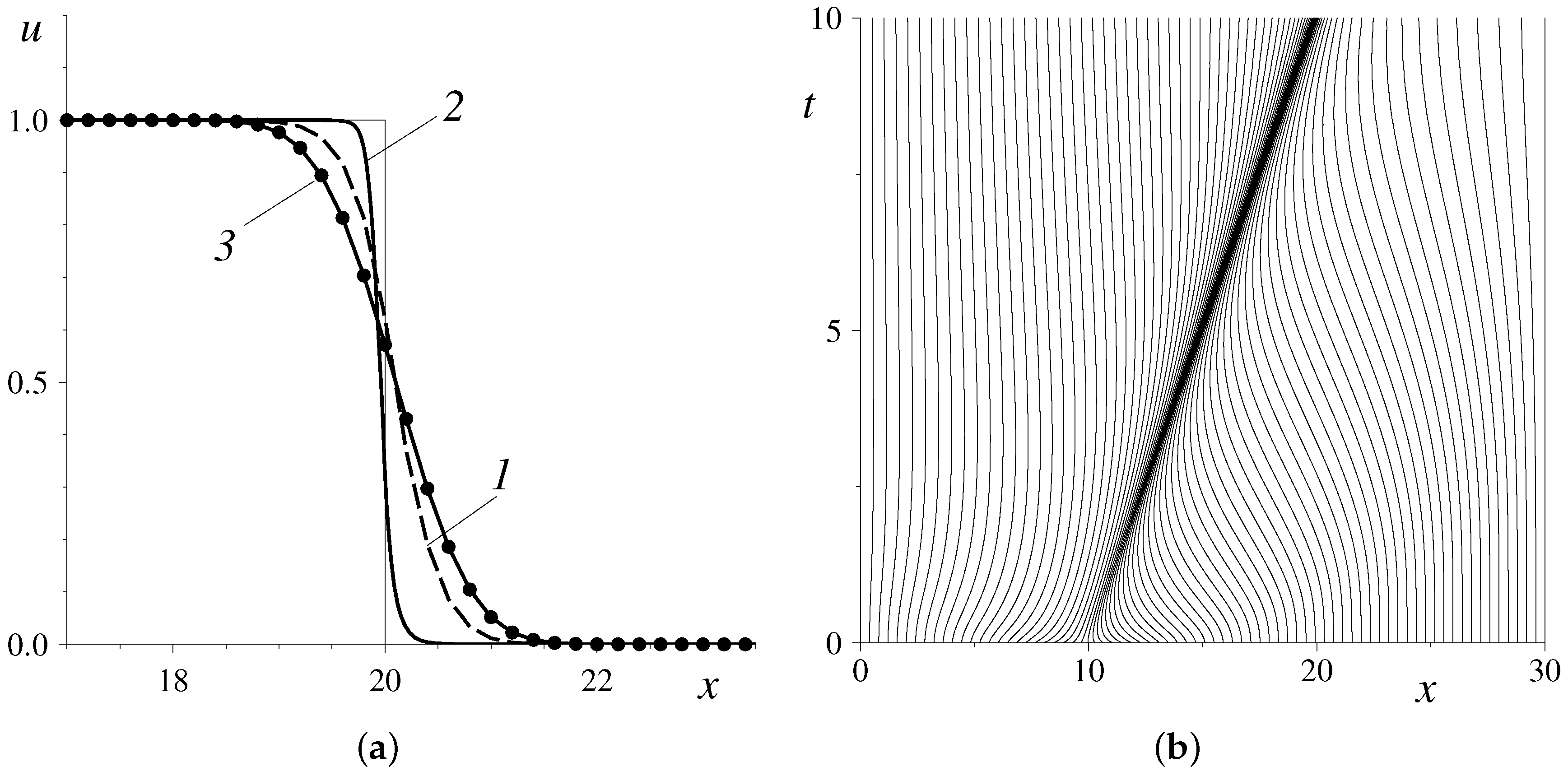
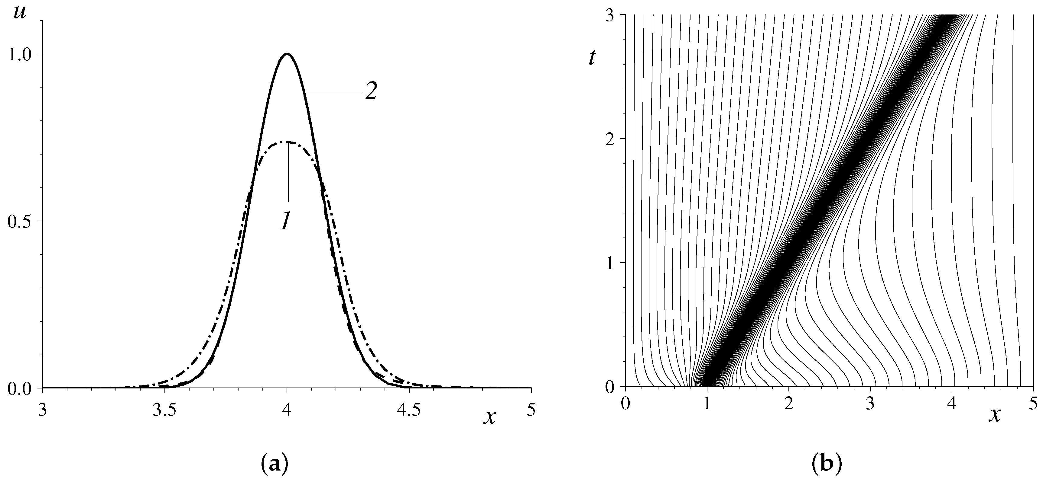
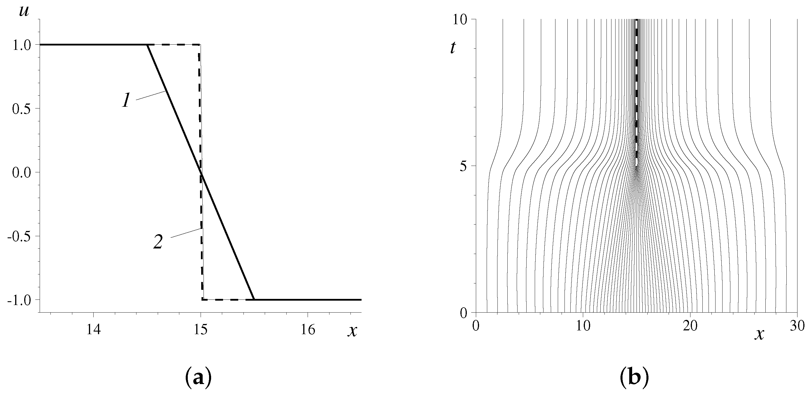
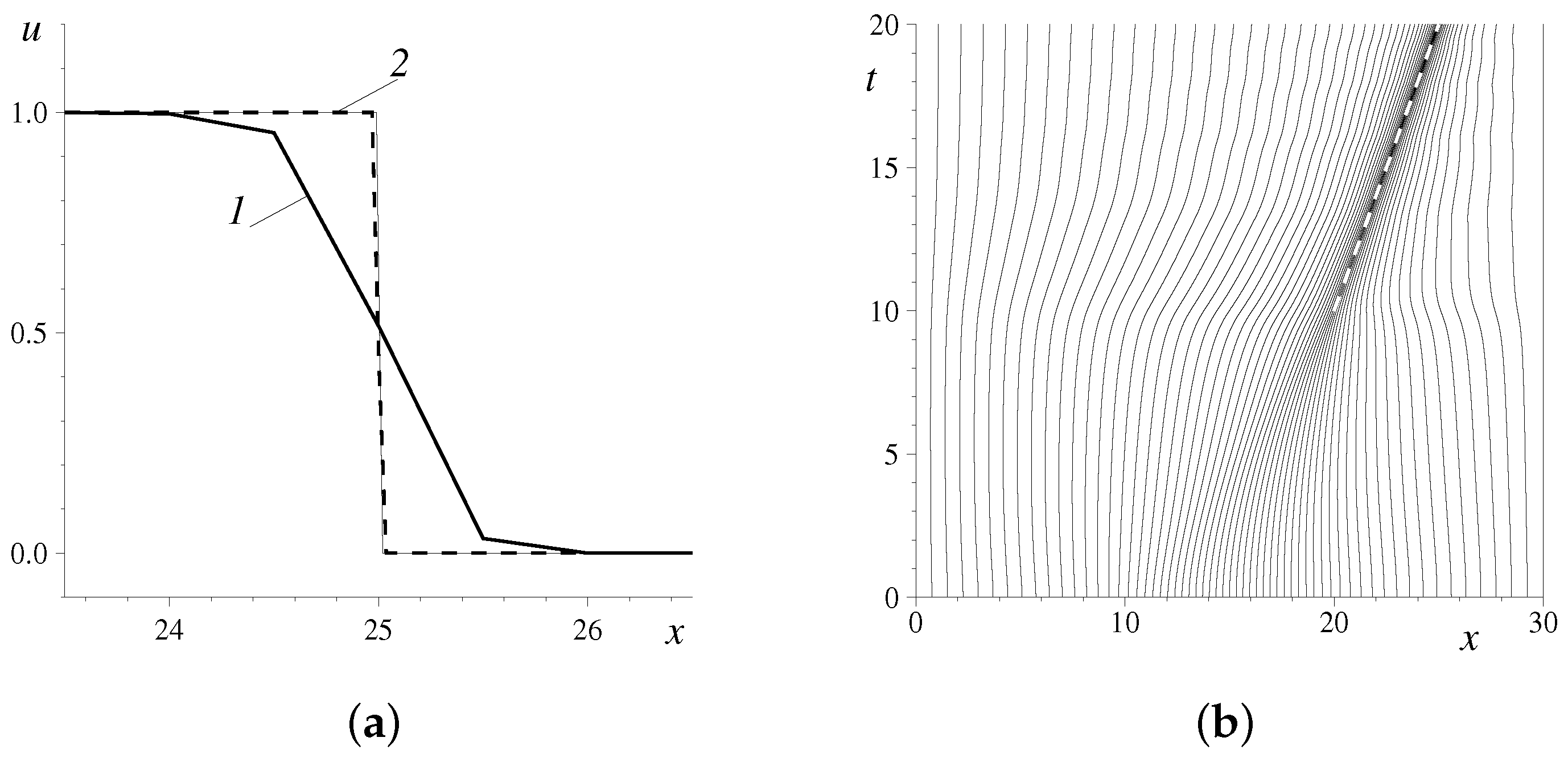
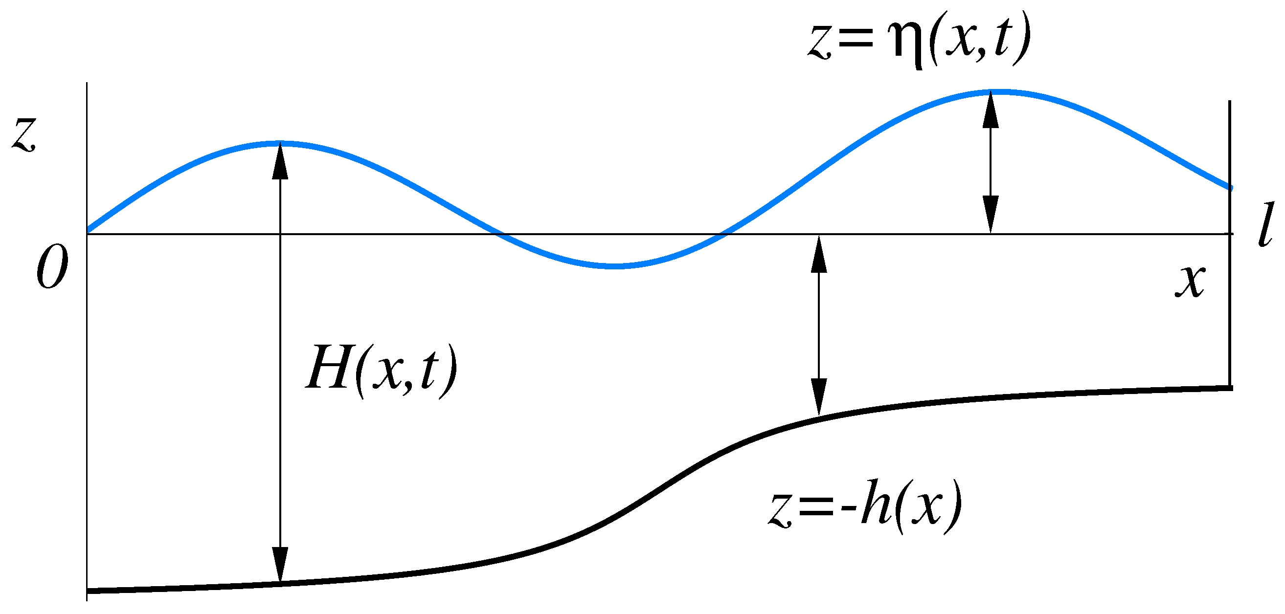
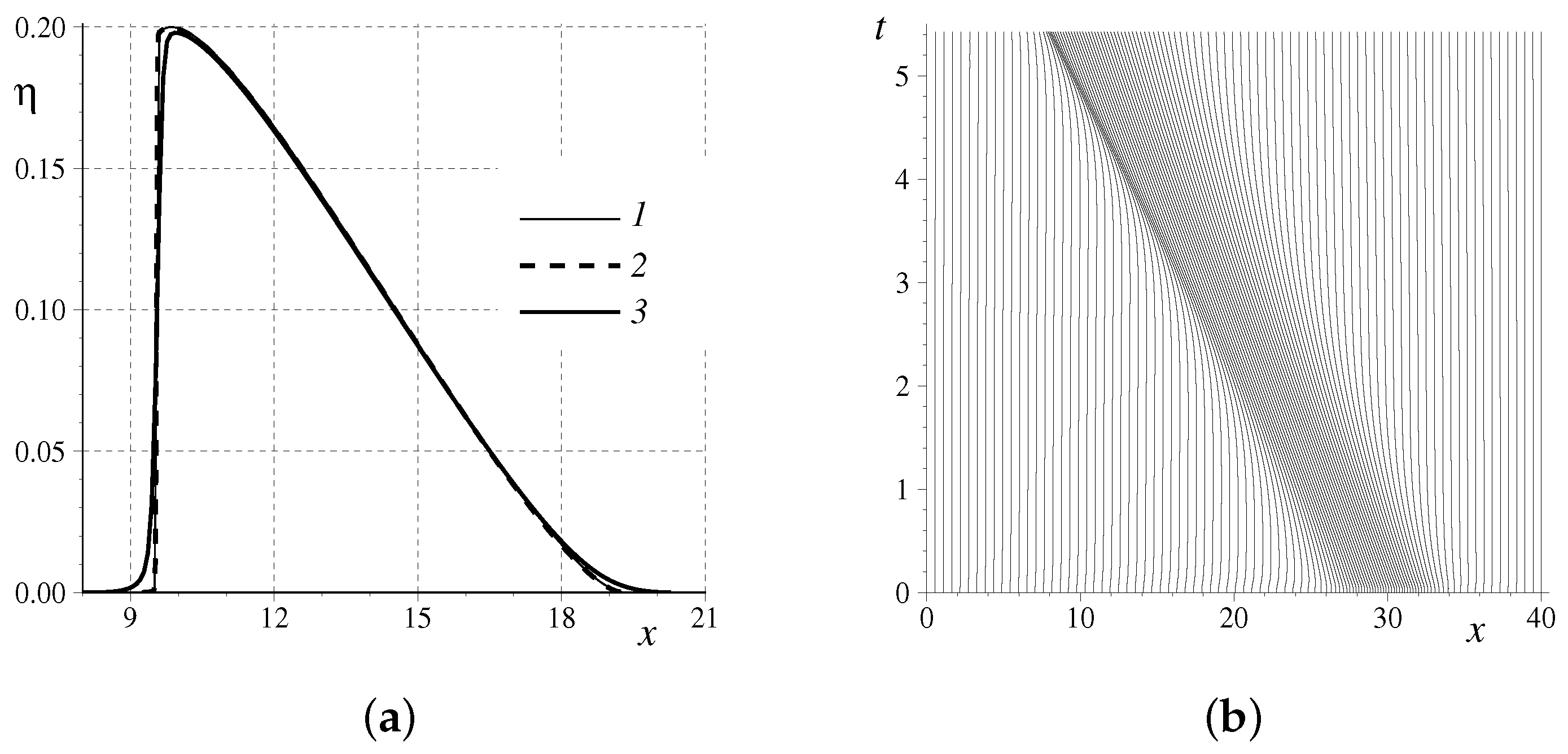
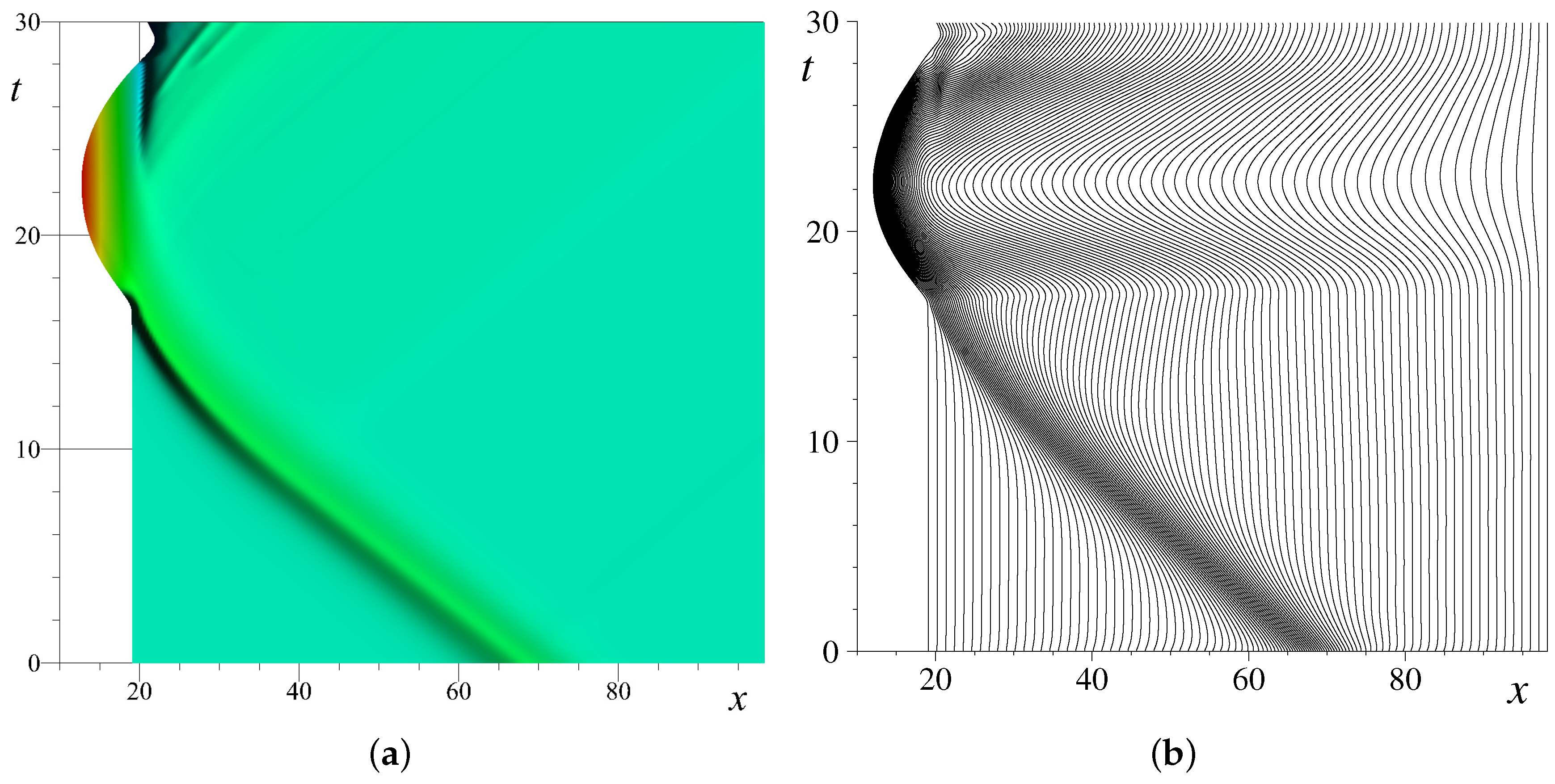
Table 1.
The numerical parameters used to simulate the discontinuous profile propagation under the linear advection of Equation (1).
Table 1.
The numerical parameters used to simulate the discontinuous profile propagation under the linear advection of Equation (1).
| Parameter | Value |
|---|---|
| Computational domain length, ℓ | |
| Number of nodes, N | 150 |
| CFL number, C | |
| Final simulation time, | |
| Propagation speed, a | |
| Initial position of the discontinuity, | |
| Monitor function parameter, | |
| Grid diffusion parameter, | |
| Smoothing parameter, |
Table 2.
The numerical parameters used to simulate the bell-shaped profile propagation under the linear advection of Equation (1).
Table 2.
The numerical parameters used to simulate the bell-shaped profile propagation under the linear advection of Equation (1).
| Parameter | Value |
|---|---|
| Computational domain length, ℓ | |
| Number of nodes, N | 150 |
| CFL number, C | |
| Final simulation time, | |
| Initial position of the bell, | |
| Propagation speed, a | |
| Monitor function parameter, | |
| Grid diffusion parameter, | |
| Smoothing parameter, |
Table 3.
The numerical parameters used to simulate a stationary shock-wave formation under the Burgers–Hopf equation dynamics.
Table 3.
The numerical parameters used to simulate a stationary shock-wave formation under the Burgers–Hopf equation dynamics.
| Parameter | Value |
|---|---|
| Computational domain length, ℓ | |
| Number of nodes, N | 60 |
| Final simulation time, | |
| CFL number, C | |
| Left transition coordinate, | |
| Right transition coordinate, | |
| Left constant state, | |
| Right constant state, | |
| Monitor function parameter, | |
| Grid diffusion parameter, | |
| Smoothing parameter, |
Table 4.
The numerical parameters used in validations of the nonlinear shallow water equations solver.
Table 4.
The numerical parameters used in validations of the nonlinear shallow water equations solver.
| Parameter | Value |
|---|---|
| Computational domain length, ℓ | |
| Number of nodes, N | 100 |
| Final simulation time, | |
| CFL number, C | |
| Gravity acceleration, g | |
| Initial wave amplitude, a | |
| Wave crest initial position, | |
| Initial wavelength, | |
| Undisturbed water depth, | |
| Monitor function parameter, | |
| Monitor function parameter, | |
| Grid diffusion parameter, | |
| Smoothing parameter, |
Table 5.
The numerical solution errors measured at the final simulation time on a fixed grid. The reference solution is given be Equations (25) and (27). All numerical parameters for this simulation are reported in Table 4.
| N | u | CPU Time, s | |||
|---|---|---|---|---|---|
| 100 | |||||
| 200 | |||||
| 400 | |||||
| 800 | |||||
| 1600 | |||||
| 3200 | |||||
| 6400 | |||||
Table 6.
The numerical solution errors measured at the final simulation time on a moving grid. The reference solution is given be Equations (25) and (27). All numerical parameters for this simulation are reported in Table 4.
| N | u | CPU Time, s | |||
|---|---|---|---|---|---|
| 100 | |||||
| 200 | |||||
| 400 | |||||
| 800 | |||||
| 1600 | |||||
| 3200 | |||||
| 6400 | |||||
Table 7.
The numerical parameters used in a solitary wave run-up simulation in nonlinear shallow water equations.
Table 7.
The numerical parameters used in a solitary wave run-up simulation in nonlinear shallow water equations.
| Parameter | Value |
|---|---|
| Computational domain length, ℓ | |
| Number of nodes, N | 1000 |
| Final simulation time, | |
| CFL number, C | |
| Gravity acceleration, g | |
| Initial wave amplitude, | |
| Wave crest initial position, | |
| Beach slope position, | |
| Beach slope, | |
| Undisturbed water depth, | |
| Monitor function parameter, | |
| Grid diffusion parameter, | |
| Smoothing parameter, |
© 2019 by the authors. Licensee MDPI, Basel, Switzerland. This article is an open access article distributed under the terms and conditions of the Creative Commons Attribution (CC BY) license (http://creativecommons.org/licenses/by/4.0/).
Share and Cite
MDPI and ACS Style
Khakimzyanov, G.; Dutykh, D.; Mitsotakis, D.; Shokina, N.Y. Numerical Simulation of Conservation Laws with Moving Grid Nodes: Application to Tsunami Wave Modelling. Geosciences 2019, 9, 197. https://doi.org/10.3390/geosciences9050197
AMA Style
Khakimzyanov G, Dutykh D, Mitsotakis D, Shokina NY. Numerical Simulation of Conservation Laws with Moving Grid Nodes: Application to Tsunami Wave Modelling. Geosciences. 2019; 9(5):197. https://doi.org/10.3390/geosciences9050197
Chicago/Turabian StyleKhakimzyanov, Gayaz, Denys Dutykh, Dimitrios Mitsotakis, and Nina Yu. Shokina. 2019. "Numerical Simulation of Conservation Laws with Moving Grid Nodes: Application to Tsunami Wave Modelling" Geosciences 9, no. 5: 197. https://doi.org/10.3390/geosciences9050197
Note that from the first issue of 2016, this journal uses article numbers instead of page numbers. See further details here.