A Study of Wave Dissipation Rate and Particles Velocity in Muddy Beds

Abstract

The interactions between free surface waves and layers of cohesive sediments including wave height attenuation and mud movement are of great importance in coastal and marine engineering. In this study, the results from a new analytical model were compared with those from literature experimental works and analytical models in terms of wave height dissipation rate and mud velocity. It was found that the new model provided good agreements in the case of coexisting waves and currents, while the literature model of Ng (explained in Section 2 of the text) —assuming the mud layer as a highly viscous layer with high shear rates—matched well with the experimental data for high viscosity (mud viscosity, ν_m = O [0.01 m²/s]). In addition, it was found that the new model is able to successfully simulate particles velocity in the presence of co-current.

1. Introduction

The interaction between waves and sediments is of great importance in the field of coastal engineering and physical oceanography. Many parts of coastal regions are covered by the cohesive sediments, in different forms, e.g., consolidated or fluidized. Wave attenuation and mud transport are two major phenomena induced by the mud mechanical responses to wave loadings. The mud particles velocity and the resultant mud transport greatly affect coastal environment and geomorphology by transporting chemical species. In addition, the mud transport is of great importance in designing the harbors and dredging systems [1]. By transferring the energy from the free surface water waves to the lower depths and consequently to the muddy bottom, the mud layer starts moving (i.e., mud transport) and the wave energy damps due to the wave induced shear effects (i.e., wave height attenuation). Such phenomenon is called wave-mud interaction.

The interaction between waves and muddy beds was widely studied using theoretical, experimental, and numerical approaches. Many analytical attempts have been made since Gade [2] to formulate the interaction of waves and muddy beds. Dalrymple and Liu [3] provided analytical solutions to formulate the wave attenuation rate and particles velocity. They applied four different assumptions, namely the complete model (CM), deep-water layer, thin lower layer (TL) and potential flow (BL). Details about these assumptions are described in Section 2 (

Table 1. List of the models considered in this study.

Model	Reference	Assumptions	Governing Equations	Dispersion Relation	Water Boundary Layer	Improvements
CM	Dalrymple and Liu [3]	Thick lower layer	Full range linearized momentum equations	implicit	Considered	Two-layer solution of Navier-Stokes equations as a first time
TL	Dalrymple and Liu [3]	Thin lower layer	Full range linearized momentum equations	implicit	Considered	Considering the thin lower layer assumptions
MP	Macpherson [4]	Thin/thick lower layer	Full range linearized momentum equations	explicit	Not Considered	Straightforward dispersion relation
Ng	Ng [5]	Thin lower layer	Boundary layer equations	explicit	Considered	Second-order solution of two-layer boundary layer equations
BL	Dalrymple and Liu [3]	Thick lower layer	Boundary layer equations/potential flows	explicit	Considered	Potential flow solutions for a thick layer of mud

and Figure 1). In their pioneering study, they investigated the first order aspects of the wave-mud interaction, such as wave height attenuation rate, particles velocity, and phase shift. However, they did not consider the mud mass transport in their study.

Macpherson [4] presented a viscoelastic model (MP), where the mudflow consisted of rotational and potential parts. Neglecting the water boundary layer, he also investigated the effects of the lower layer elasticity on the wave damping. However, he neither provided the results for his general proposed dispersion relation nor verified his analytical results for the velocity amplitudes.

Ng [5] presented an asymptotic solution to the two-layer Stokes boundary layer water–mud problem (Ng). He derived direct solutions for the particles velocity, dissipation rate, and phase shift at the first order, and water and mud mass transport velocity at the second order. Liu and Chan [6] presented a new model on wave attenuation assuming that the thickness of the mud layer is of the same order of magnitude as the boundary layer thickness. They applied their model to a viscoelastic muddy bed and discussed the wave attenuation rate, water–mud interfacial interaction, velocity profile, effects of viscosity and the impacts of elasticity. Their theoretical results were successfully compared with available experimental data and other existing numerical results. Kranenburg et al. [7] implemented a new dispersion relation obtained from a viscous two-layer model in the wave-forecasting model, SWAN, to simulate wave damping in coastal areas by fluid mud deposits. The dispersion relation was derived for a viscous layer overlying by an inviscid upper layer. Assessing the two-dimensional evolution of wave fields in coastal areas, they showed that their new model could be applied to natural conditions. All of the models as well as a sketch of their assumptions (CM, BL, Ng, TL, and MP) are further described and presented in more details in Section 2.

In addition to the analytical studies, few experimental studies were carried on the wave attenuation rates and mud transport. Sakakiyama and Bijker [8] presented experimental investigations of the soft mud interacting with the overlying water layer. They performed their experiments on viscoelastic mud layer and compared the results with a proposed theoretical solution. They did not measure the particles velocity and so the values of their proposed analytical model could not be investigated. However, they measured the mass transport velocities using a tracer. Since then, few more laboratory experiments were carried to measure the dissipation rates and mass transport (e.g., [2,9,10]). Recently, Hsu et al. [10], and Soltanpour et al. [11] applied electromagnetic current meters in the mud layer and investigated the mud particles velocity and mass transport using commercial kaolinite as the mud bed. They successfully measured the time-dependent instantaneous velocity inside the mud layer, however, Hsu et al. [10] did not provide information on the resultant mud mass transport velocity.

Few numerical studies on wave–mud interaction have been reported in the literature. Zhang and Ng [12] presented a numerical model for a two-layer viscous fluid system to simulate a progressive wave in the upper layer and the oscillatory motion of lower mud layer induced by the water wave to evaluate the ratio of interfacial to surface wave amplitude. Niu and Yu [13] developed a numerical model using a finite difference scheme, in which the motions of the movable mud and water were solved simultaneously. A visco-elastic–plastic model was considered for the mud layer. The free surface and the water–mud interface were both traced by the method of volume of fluid (VOF). They achieved good agreements with the measurements in the case of constant topography. Hejazi et al. [14] applied the full ranges of Navier-Stokes equations with a complete set of kinematic and dynamic boundary conditions at free surface and interface and the two-equation standard k-ε turbulence model with buoyancy terms. The finite volume method based on an ALE description was utilized for the simulation of wave motion in a combined system of water and viscous mud layer. Beyramzadeh and Siadatmousavi [15] successfully extended the SWAN wave model to include attenuation of the wave energy due to interaction with a viscoelastic fluid mud layer. The performances of implemented viscoelastic models were verified against an analytical solution and viscous formulations for simple one-dimensional propagation cases.

An investigation of the existing analytical models with their different assumptions, and comparisons of the particles velocity and wave height dissipation with laboratory experiments in the wave-mud interaction have not been carried so far. The present study compares the literature models (Table 1, Section 2) in terms of dissipation rate, particles velocity and mass transport. The studies of Kranenburg et al. [7], and Liu and Chan [6] were excluded since the former’s assumption is similar to that of Ng [5], however, they neglected the water boundary layer, and the latter provided a viscoelastic model, which is beyond the scope of the present study. A new model with a direct formulation of dispersion relation for the pure wave and wave–current–mud interaction is also proposed. Thereafter, the effects of current on the wave-mud interaction, e.g., wave attenuation and particles velocity, is addressed. The results of the literature models together with the current model are compared with the experimental results of Soltanpour et al. [11]. The performance of the models in different cases are compared and discussed.

2. Analytical Models

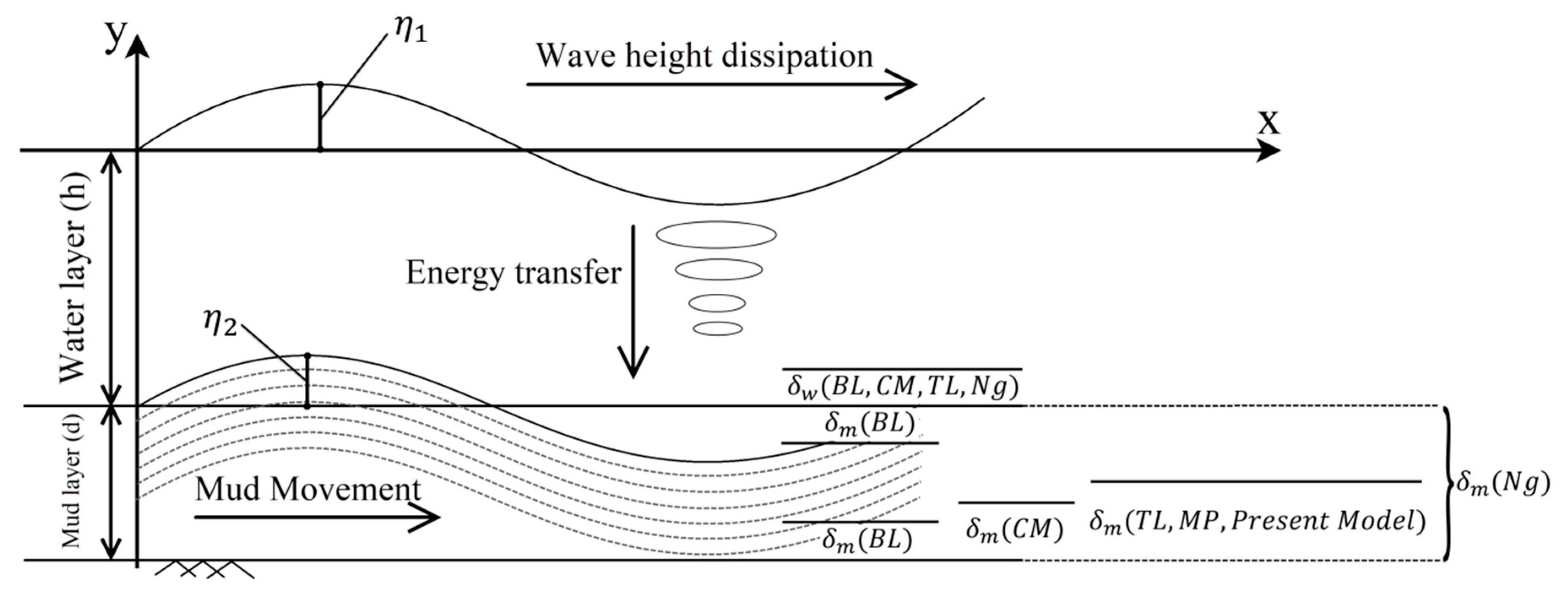
In this section, the Complete model (CM), the thin lower layer model (TL), the Macpherson model (MP), the two-layer Stokes boundary layer model (Ng), and the potential flow model (BL) are presented. Figure 1 provides a sketch of the wave-mud interaction, where δ is the Stokes boundary layer thickness (${\delta }_{w,m}=\sqrt{\frac{2{\nu }_{w,m}}{\sigma }}$, where, ν and σ are the kinematic viscosity and wave angular frequency respectively, and w, m denote water and mud, respectively), η₁ and η₂ are the free surface and interface amplitudes, x and y are the horizontal and vertical coordinates, respectively.

Table 1 summarizes the analytical models of Dalrymple and Liu [3], Macpherson [4], and Ng [5] with their assumptions, equations and solutions.

The mud layer was considered as fully homogeneous and fluidized and subsequently, the Newtonian rheological model was applied in all of the discussed models as well as the present model. A train of regular waves is traveling on a water surface overlying a fluid mud layer. In the models, ρ is the density, $\nu$ the dynamic viscosity, h the water depth, and d is the mud thickness. The free surface (η₁) and interface displacements (η₂) are expressed as Equations (1) and (2), respectively

$${\eta }_1=a{e}^{i\left(kx-\sigma t\right)}$$

(1)

$${\eta }_2=b{e}^{i\left(kx-\sigma t\right)}$$

(2)

where k is the wave number.

2.1. A Review on the Analytical Models

2.1.1. COMPLETE MODEL

Neglecting the second order advection terms, the full range Navier-Stokes equations were solved by applying the appropriate dynamic and kinematic boundary conditions at the water free surface, water-mud interface, and the rigid bottom. Each of the viscous effects in the equations was assumed to be effective close to the corresponding boundaries, i.e., rigid, interface, and free surface boundaries.

The linearized Navier-Stokes equations governing the two-layer system of the water and mud are

$$\frac{\partial {\tilde{u}}_f}{\partial t}=-\frac{1}{{\rho }_f}\frac{\partial {\tilde{p}}_f}{\partial x}+{\nu }_f\left(\frac{{\partial }^2{\tilde{u}}_f}{\partial x^2}+\frac{{\partial }^2{\tilde{u}}_f}{\partial y^2}\right)$$

(3)

$$\frac{\partial {\tilde{v}}_f}{\partial t}=-\frac{1}{{\rho }_f}\frac{\partial {\tilde{p}}_f}{\partial y}+{\nu }_f\left(\frac{{\partial }^2{\tilde{v}}_f}{\partial x^2}+\frac{{\partial }^2{\tilde{v}}_f}{\partial y^2}\right)$$

(4)

where $\tilde{u}$, $\tilde{v}$ are the horizontal and vertical velocities corresponding to the x and y directions respectively, $\tilde{p}$ is the dynamic pressure, and t represents the time.

The continuity equation is also written as

$$\frac{\partial {\tilde{u}}_f}{\partial x}+\frac{\partial {\tilde{v}}_f}{\partial y}=0$$

(5)

The variables were separated into periodic and stationary terms as follows

$${\tilde{u}}_f=u_f\left(y\right)e^{i\left(kx-\sigma t\right)}$$

(6)

$${\tilde{v}}_f=v_f\left(y\right)e^{i\left(kx-\sigma t\right)}$$

(7)

$${\tilde{p}}_f=p_f\left(y\right)e^{i\left(kx-\sigma t\right)}$$

(8)

where, $u$ and $v$ are amplitudes of the horizontal and vertical velocities, respectively, and p is the dynamic pressure amplitude. Substitution of the Equations (6)–(8) into the momentum Equations (3) and (4) and replacing the pressure and horizontal velocity by the vertical velocity using continuity equation (Equation (5)) resulted in the following ordinary differential equation ([3])

$$v_f^{⁗}-\left(k^2+{\lambda }_f^2\right)v_f^{″}+k^2{\lambda }_f^2{v}_f=0$$

(9)

where, ${\lambda }_f^2=k^2-i\sigma /{\nu }_f$.

By using the method of characteristic, the complete solution of the governing differential equation (Equation (9)) was

$$v_w=A_w\sinh k\left(h+y\right)+B_w\cosh k\left(h+y\right)+C_w{e}^{{\lambda }_{w}y}+D_w{e}^{-{\lambda }_w\left(h+y\right)}$$

(10)

$$v_m=A_m\sinh k\left(h+y\right)+B_m\cosh k\left(h+y\right)+C_m{e}^{{\lambda }_m\left(h+y\right)}+D_m{e}^{-{\lambda }_m\left(h+y+d\right)}$$

(11)

where A-D are constant coefficients obtained from the boundary conditions. Substituting Equations (10), (11) into the continuity equation (Equation (5)), the following expressions for the horizontal velocities were obtained

$$u_w=i\left[A_w\cosh k\left(h+y\right)+B_w\sinh k\left(h+y\right)+C_w\frac{{\lambda }_w}{k}{e}^{{\lambda }_{w}y}-D_w\frac{{\lambda }_w}{k}{e}^{-{\lambda }_w\left(h+y\right)}\right]$$

(12)

$$\begin{array}{ll}{u}_m=& i[A_m\cosh k\left(h+y+d\right)+B_m\sinh k\left(h+y+d\right)+C_m\frac{{\lambda }_m}{k}{e}^{{\lambda }_m\left(h+y\right)}\\ & -D_m\frac{{\lambda }_m}{k}{e}^{-{\lambda }_m\left(h+y+d\right)}]\end{array}$$

(13)

The water–mud system of equations contain 10 unknowns (eight coefficients, A_w-D_w, A_m-D_m, together with the wave number, k, and the water–mud interface amplitude, b). Thus, 10 boundary conditions (including kinematic and dynamic boundary conditions, i.e., no slip condition at the bottom, continuity of velocities and stresses at the interface, sharp interface at the free surface, and zero stress and pressure at the free surface) were taken into account as follows (for more details, please refer to Dalrymple and Liu [3])

$${\tilde{v}}_m=0, y=-h-d$$

(14)

$${\tilde{u}}_m=0, y=-h-d$$

(15)

$$\frac{\partial {\eta }_2}{\partial t}={\tilde{v}}_w, y=-h$$

(16)

$${\tilde{v}}_w={\tilde{v}}_m, y=-h$$

(17)

$${\tilde{u}}_w={\tilde{u}}_m, y=-h$$

(18)

$${\tilde{p}}_w-2{\rho }_w{\nu }_w\frac{\partial {\tilde{v}}_w}{\partial y}-{\rho }_{w}g{\eta }_2={\tilde{p}}_m-2{\rho }_m{\nu }_m\frac{\partial {\tilde{v}}_m}{\partial y}-{\rho }_{m}g{\eta }_2, y=-h$$

(19)

$${\rho }_w{\nu }_w\left(\frac{\partial {\tilde{u}}_w}{\partial y}+\frac{\partial {\tilde{v}}_w}{\partial x}\right)={\rho }_m{\nu }_m\left(\frac{\partial {\tilde{u}}_m}{\partial y}+\frac{\partial {\tilde{v}}_m}{\partial x}\right), y=-h$$

(20)

$$\frac{\partial {\eta }_1}{\partial t}={\tilde{v}}_w, y=0$$

(21)

$${\tilde{p}}_w-2{\rho }_w{\nu }_w\frac{\partial {\tilde{v}}_w}{\partial x}-{\rho }_{w}g{\eta }_1=0, y=0$$

(22)

$${\rho }_w{\nu }_w\left(\frac{\partial {\tilde{u}}_w}{\partial y}+\frac{\partial {\tilde{v}}_w}{\partial x}\right)=0, y=0$$

(23)

Substituting Equations (6)–(8) into the boundary conditions (14)–(23), the original form of the boundary conditions reduces to Equations (A1)–(A10). Details are provided in Appendix A.

Thin Lower Layer (TL).

Since the fluid mud is assumed as a thin layer, the only difference between TL and CM models is that in the TL model, the third and fourth terms (viscous effects) at the right hand sides of Equations (10), (11) are effective over the entire depth of fluid mud.

According to the above assumptions, the following solutions were obtained [3]

$$v_w=A_w\sinh k\left(h+y\right)+B_w\cosh k\left(h+y\right)+C_w{e}^{{\lambda }_{w}y}+D_w{e}^{-{\lambda }_w\left(h+y\right)}$$

(24)

$$\begin{array}{ll}{v}_m=& A_m\sinh k\left(h+y+d\right)+B_m\cosh k\left(h+y+d\right)+C_m\sinh {\lambda }_m\left(h+y+d\right)\\ & +D_m\cosh {\lambda }_m\left(h+y+d\right)\end{array}$$

(25)

where the related boundary conditions (Equations (14)–(23)) converted to A11–A20 (Appendix A). The solution procedure was the same as the CM model.

2.1.2. MACPHERSON MODEL

In this model, the lower viscoelastic layer (mud) was divided into a rotational part and a potential part, while the upper layer (clear water) is inviscid. This is similar to the thin lower layer proposed by Dalrymple and Liu [3]. However, the upper layer boundary layer was not neglected in the TL model, which resulted in implicit dispersion relation. Macpherson [4] proposed a straightforward dispersion relation by substituting the boundary conditions. He presented two slow and fast mode solutions of the dispersion relation in the case of deep lower layer ($d\to \infty$). Here, the elasticity is neglected and the mud is considered as a viscous layer.

Considering the mud flow consists of the two parts (rotational and potential), the following relations were obtained ([4,5])

$${\nabla }^2{\varnothing }_w=0,-h<y<0$$

(26)

$${\nabla }^2{\varnothing }_m=0,-(h+d)<y<-h$$

(27)

$${\mathsf{\nu }}_m{\nabla }^2{\psi }_m=\frac{\partial {\psi }_m}{\partial t}$$

(28)

$$u_m=-\frac{\partial {\varnothing }_m}{\partial x}-\frac{\partial {\psi }_m}{\partial y}$$

(29)

where ${\varnothing }_f$ is the velocity potential of the flow in the water and mud layers, and ${\psi }_m$ the stream function in the mud layer.

Applying the appropriate kinematic and dynamic boundary conditions (Equations (30)–(36)), the dispersion relation was obtained (Equation (37))

$$-\frac{\partial {\varnothing }_m}{\partial y}+\frac{\partial {\psi }_m}{\partial x}=0, y=-h-d$$

(30)

$$-\frac{\partial {\varnothing }_m}{\partial x}-\frac{\partial {\psi }_m}{\partial y}=0, y=-h-d$$

(31)

$${\tilde{p}}_m-2{\rho }_m{\nu }_m\frac{\partial {\tilde{v}}_m}{\partial y}={\tilde{p}}_w, y=-h$$

(32)

$${\rho }_{\mathrm{m}}{\nu }_{\mathrm{m}}\left(-2\frac{{\partial }^2{\varnothing }_m}{\partial x\partial y}-\frac{{\partial }^2{\psi }_m}{\partial y^2}-\frac{{\partial }^2{\psi }_m}{\partial x^2}\right)=0, y=-h$$

(33)

$$\frac{\partial {\eta }_2}{\partial t}=-\frac{\partial {\varnothing }_w}{\partial y}, y=-h$$

(34)

$$-\frac{\partial {\varnothing }_m}{\partial y}+\frac{\partial {\psi }_m}{\partial x}=-\frac{\partial {\varnothing }_w}{\partial y}, y=-h$$

(35)

$$\frac{\partial {\eta }_1}{\partial t}=-\frac{\partial {\varnothing }_w}{\partial y}, y=0$$

(36)

$$\frac{{\partial }^2{\varnothing }_w}{\partial t^2}+g\frac{\partial {\psi }_w}{\partial y}=0, y=0$$

(37)

$$\begin{array}{ll}\frac{{\rho }_w\left[{\sigma }^4-g^2{k}^2\right]\tanh kh}{gk\tanh kh-{\sigma }^2}+{\rho }_{m}gk& \\ & +{\rho }_m{\left(2k^2{\nu }_m-i\sigma \right)}^2\left\{\frac{\left(2k^2-i\sigma /{\nu }_m\right)\left[{\lambda }_{m}C{H}_{k}C{H}_l-kS{H}_{k}S{H}_l\right]-2k^2{\lambda }_m}{\left(2k^2-i\sigma /{\nu }_m\right)\left[{\lambda }_{m}S{H}_{k}C{H}_l-kC{H}_{k}S{H}_l\right]}\right\}\\ & -4{\rho }_m{\lambda }_m{k}^3{\nu }_m{}^3\left\{\frac{\left(2k^2-i\sigma /{\nu }_m\right)-2k\left[kC{H}_{k}C{H}_l-{\lambda }_{m}S{H}_{k}S{H}_l\right]}{2k\left[{\lambda }_{m}S{H}_{k}C{H}_l-kC{H}_{k}S{H}_l\right]}\right\}=0\end{array}$$

(38)

where $C{H}_k=\cosh kd$, $S{H}_k=\sinh kd$, $C{H}_{\mathrm{l}}=\cosh {\lambda }_{m}d$, $S{H}_{\mathrm{l}}=\sinh {\lambda }_{m}d$.

The dispersion relation (Equation (38)) resulted in two different solutions for the fast and slow modes.

2.1.3. TWO-LAYER STOKES BOUNDARY LAYER MODEL

Ng [5] developed an asymptotic theory for the flow kinematics of a thin layer of viscous mud under surface water waves. The mud depth, the thickness of Stokes’ boundary layer in the mud layer, and the wave amplitude were assumed to be comparable with one another, and much smaller than the wavelength. Ng [5] did not consider the effects of the core region (inviscid flow) in his model, which is its main difference with the TL model. Using a sharp contrast in length scales, boundary layer equations were used to describe the motion of both the mud and immediately overlying water. Explicit expressions were obtained for the fluid velocity field, interface wave characteristics, and wave-damping rate at the first-order, as well as the steady mean discharge rate, and mud mass-transport velocity at the second-order, under progressive waves. Solving the first order Navier-Stokes equations, Ng [5] obtained the relations for oscillating velocities inside the mud and water boundary layers

$$u_w=\left(1+D_{w,ng}{e}^{-{\lambda }_{wng}\left(h+y\right)}\right)U_{p,w}$$

(39)

$$u_m=\left[\gamma +C_{m,ng}\cosh {\lambda }_{mng}\left(h+y+d\right)+D_{m,ng}\sinh {\lambda }_{mng}\left(h+y+d\right)\right]U_{p,w}$$

(40)

where D_m,ng, C_m,ng, and D_m,ng are the coefficients defined in Ng (2000), $U_{p,w}$ the inviscid velocity at the interface of the water and mud layers, and ${\lambda }_{w,mng}=\left(1-i\right)\sqrt{\sigma /2{\nu }_{w,m}}$, and $\gamma =\frac{{\rho }_w}{{\rho }_m}$.

Ng [5] also presented a direct relation for the dissipation rate. Since the assumption implied that the fluid mud layer was considered as highly viscous, the effects of stratification on the dispersion relation was not considered and the fast mode was the only governing mode. By taking the time average of the second order equations of Navier-Stokes, he obtained the mass transport velocity inside the water and mud as:

$${\overline{u}}_{mL}\left(n_n\right)=k{\sigma }^{-1}{\left|U_{p,w}\right|}^2\left[F_m\left(n_n\right)+CO{F}_m{n}_n+F_{m1}\left(n_n\right)+F_{m2}\left(n_n\right)\right] in 0<n_n<d_n$$

(41)

$${\overline{u}}_{wL}\left(n_n\right)=k{\sigma }^{-1}{\left|U_{p,w}\right|}^2\left[F_w\left(n_n\right)+CO{F}_w+F_{w1}\left(n_n\right)+F_{w2}\left(n_n\right)\right] in d_n<n_n<\infty$$

(42)

where, ${\overline{u}}_{mL}$, ${\overline{u}}_{wL}$ are the mass transport velocities inside the mud and water, respectively, $n_n$ is the dimensionless form of the depth, i.e. $n_n=\left(y+h+d\right)\sqrt{\sigma /2{\nu }_m}$, and $d_n=d\sqrt{\sigma /2{\nu }_m}$ is the dimensionless mud thickness. The other parameters of $CO{F}_m$, $CO{F}_w$, $F_m$, $F_w$, $F_{m1}$, $F_{m2}$, $F_{w1}$ and $F_{w2}$ were defined in details in Ng [5].

2.1.4. POTENTIAL FLOWS

The mud layer was considered thick enough such that the viscous effects dominate only closer to the boundaries, while the whole layer is affected by the potential flow. In addition, the water layer is affected by the viscous terms close to the interface boundary layer and the potential flow influences the whole water layer.

The governing equations of water–mud system consist of two parts, the potential flow and the viscous boundary layers ([4,5])

$${\nabla }^2{\varnothing }_w=0,-h<y<0$$

(43)

$${\nabla }^2{\varnothing }_m=0,-(h+d)<y<-h$$

(44)

$$\frac{\partial U_f}{\partial t}={\nu }_f\frac{{\partial }^2{U}_f}{\partial y^2}$$

(45)

where, $\varnothing$ is the potential, and $U_f=u_f-U_{p,f.}$

Following the boundary conditions provided in Dalrymple and Liu [3], the velocity potential was obtained in terms of the wave number k as

$${\varnothing }_w=\left(-iag/\sigma \right)\left[\left({\sigma }^2/gk\right)\sinh ky+\cosh ky\right]e^{i\left(kx-\sigma t\right)}$$

(46)

$${\varnothing }_m=\left(-iag/\sigma \right)\left(\cosh kh/\sinh kd\right)\cosh k\left(h+y+d\right)\left[\left({\sigma }^2/gk\right)-\tanh kh\right]e^{i\left(kx-\sigma t\right)}$$

(47)

The kinematic boundary conditions at the rigid bottom, interface, and water free surface, and the dynamic boundary condition at the free surface, were all substituted into the dynamic boundary condition at the water–mud interface, and as a result the following was obtained

$$A{T}^2+BT+C=0$$

(48)

where, $T=\frac{{\sigma }^2}{gk}$, and,

$$\begin{gathered} A={\rho }_w\sinh kh+{\rho }_m\cosh kh\coth kd, \\ B=\left({\sigma }^2/gk\right)\left[-{\rho }_w\cosh kh-{\rho }_m\sinh kh\coth kd+\left({\rho }_w-{\rho }_m\right)\cosh kh\right], \\ C=\left[\left({\rho }_m-{\rho }_w\right)\sinh kh\right] \end{gathered}$$

The dispersion relation read as

$$\frac{{\sigma }^2}{gk}=\frac{-B\pm {\left(B^2-4AC\right)}^{1/2}}{2A}$$

(49)

where the “−” and “+” refers to the fast and slow modes respectively.

The rotational flow was obtained close to the rigid bottom ($U_3$), adjacent to the water–mud interface in the mud layer ($U_2$), and adjacent to the water–mud interface in the water layer ($U_1$) as ([3])

$$U_3=C_{m1}{e}^{-\left(1+i\right){\left(\sigma /2{\nu }_m\right)}^{1/2}\left(y+h+d\right)}$$

(50)

$$U_2=C_{m2}{e}^{\left(1+i\right){\left(\sigma /2{\nu }_m\right)}^{1/2}\left(y+h\right)}$$

(51)

$$U_1=C_{m2}{e}^{-\left(1+i\right){\left(\sigma /2{\nu }_m\right)}^{1/2}\left(y+h\right)}$$

(52)

where, $C_{m1}=-\frac{gak}{\sigma }\frac{\cosh kh}{\sinh kd}\left(\frac{{\sigma }^2}{gk}-\tanh kh\right)$, $C_{w1}=-\frac{gak}{\sigma \sinh kh}\frac{\left[\left({\rho }_m/{\rho }_w\right){\left({\nu }_m/{\nu }_w\right)}^{1/2}\right]}{\left[1+\left({\rho }_m/{\rho }_w\right){\left({\nu }_m/{\nu }_w\right)}^{1/2}\right]}\left\{\left({\sigma }^2/gk\right)-\left(1/2\right)\sinh 2kh\left[\coth kh+\coth kd\right]\left[\left({\sigma }^2/gk\right)-\tanh kh\right]\right\}$, $C_{m2}=-\left({\rho }_m/{\rho }_w\right){\left({\nu }_m/{\nu }_w\right)}^{1/2}{C}_{w1}$.

2.2. Proposed Model

The proposed model provides a direct formulation of the dispersion relation and particle velocities in both cases of pure wave and wave–current interaction. The straightforward formulation could be used in modeling a two-layer wave-mud interaction in the existence of a dense highly viscous mud layer. The model is based upon the following assumptions:

• The mud is assumed as a thin viscous layer which is comparable with TL, while the overlying water is considered as an inviscid layer.
• The current is assumed to be uniform and steady.

2.2.1. Wave-Mud Interaction

The following solutions of the momentum equations in water and mud layers (Equations (3)–(5)) are applied

$$v_w=A_w\sinh k\left(h+y\right)+B_w\cosh k\left(h+y\right)$$

(53)

$$\begin{array}{ll}{v}_m=& A_m\sinh k\left(h+y+d\right)+B_m\cosh k\left(h+y+d\right)+C_m\sinh {\lambda }_m\left(h+y+d\right)\\ & +D_m\cosh {\lambda }_m\left(h+y+d\right)\end{array}$$

(54)

which are subjected to the appropriate boundary conditions followed by TL, with neglecting the water boundary layer. Thus, the water–mud system of equations contains eight unknowns (six coefficients together with the wave number, k, and the water–mud interface amplitude, b). Thus, eight boundary conditions (including kinematic and dynamic boundary conditions, presented in detail by Dalrymple and Liu [3]) are written as

$${\tilde{v}}_m=0, y=-h-d$$

(55)

$${\tilde{u}}_m=0, y=-h-d$$

(56)

$${\tilde{p}}_m-2{\rho }_m{\nu }_m\frac{\partial {\tilde{v}}_m}{\partial y}={\tilde{p}}_w, y=-h$$

(57)

$${\rho }_{\mathrm{m}}{\nu }_{\mathrm{m}}\left(\frac{\partial {\tilde{u}}_m}{\partial y}+\frac{\partial {\tilde{v}}_m}{\partial x}\right)=0, y=-h$$

(58)

$$\frac{\partial {\eta }_2}{\partial t}={\tilde{v}}_w, y=-h$$

(59)

$${\tilde{v}}_m={\tilde{v}}_w, y=-h$$

(60)

$$\frac{\partial {\eta }_1}{\partial t}={\tilde{v}}_w, y=0$$

(61)

$${\tilde{p}}_w-2{\rho }_w{\nu }_w\frac{\partial {\tilde{v}}_w}{\partial y}-{\rho }_{w}g{\eta }_1=0, y=0$$

(62)

Substituting the velocities and dynamic pressure (Equations (6)–(8)) we will obtain the following relations

$$B_m+D_m=0$$

(63)

$$A_m+{\lambda }_m{C}_m=0$$

(64)

$$-i\sigma b=B_w$$

(65)

$$B_w=A_m\sinh kd+B_m\cosh kd+C_m\sinh {\lambda }_{m}d+D_m\cosh {\lambda }_{m}d$$

(66)

$$\begin{array}{ll}0=& {\rho }_m{\nu }_m[2k^2{A}_m\sinh kd+2k^2{B}_m\cosh kd+\left(k^2+{\lambda }_m^2\right)C_m\sinh {\lambda }_{m}d\\ & +\left(k^2+{\lambda }_m^2\right)D_m\cosh {\lambda }_{m}d]\end{array}$$

(67)

$$-i\sigma a=A_w\sinh kh+B_w\cosh kh$$

(68)

$$\frac{i{\rho }_w\sigma }{k}\left(A_w\cosh kh+B_w\sinh kh\right)-{\rho }_{w}ga=0$$

(69)

$$\begin{array}{ll}\frac{i{\rho }_w\sigma }{k}{A}_w=& M_m\left[A_m\cosh kd+B_m\sinh kd\right]-2{\rho }_m{\nu }_m{\lambda }_m\left(C_m\cosh {\lambda }_{m}d+D_m\sinh {\lambda }_{m}d\right)\\ & -\left({\rho }_m-{\rho }_w\right)gb\end{array}$$

(70)

Considering Equations (63)–(69), the coefficients, A_w, B_w, A_m, B_m, C_m,and D_m are obtained in terms of the wave number, k (see Appendix B). By substitution of the coefficients into Equation (70), the dispersion relation is found as

$$\begin{array}{l}\frac{{\rho }_m\left(\sigma +2i{k}^2{\nu }_m\right)\left[\left(k^2+{\lambda }_m^2\right)\left(kS{H}_{k}S{H}_l-{\lambda }_{m}C{H}_{k}C{H}_l+2k^2{\lambda }_m\right)\left(gkS{H}_h\right)-{\sigma }^{2}C{H}_h\right]}{k\sigma \left(k-{\lambda }_m\right)\left(k+{\lambda }_m\right)\left(kC{H}_{k}S{H}_l-{\lambda }_{m}S{H}_{k}C{H}_l\right)}\\ -\frac{2ik{\mathsf{\lambda }}_m{\nu }_m{\rho }_m\left(2k^{2}C{H}_{k}C{H}_l-2k{\lambda }_{m}S{H}_{k}S{H}_l-k^2-{\lambda }_m^2\right)\left(gkS{H}_h-{\sigma }^{2}C{H}_h\right)}{\mathsf{\sigma }\left(k^2-{\lambda }_m^2\right)\left(kC{H}_{k}S{H}_l-{\lambda }_{m}S{H}_{k}C{H}_l\right)}\\ +\frac{g\left({\rho }_w-{\rho }_m\right)\left({\sigma }^{2}C{H}_h-gkS{H}_h\right)}{{\sigma }^2}+\frac{{\rho }_{w}S{H}_h\left[{\sigma }^2-gk\coth \left(kh\right)\right]}{k}=0\end{array}$$

(71)

where $C{H}_h=\cosh kh$ and SH_h = sinh kh.

2.2.2. Wave–Current Interaction

Governing Equations

Applying the assumptions mentioned above, the governing equations for the wave–current–mud interaction are [17]

$$\frac{\partial {\tilde{u}}_w}{\partial t}+U_c\frac{\partial {\tilde{u}}_w}{\partial x}=-\frac{1}{{\rho }_w}\frac{\partial {\tilde{p}}_w}{\partial x}$$

(72)

$$\frac{\partial {\tilde{v}}_w}{\partial t}+U_c\frac{\partial {\tilde{v}}_w}{\partial x}=-\frac{1}{{\rho }_w}\frac{\partial {\tilde{p}}_w}{\partial z}$$

(73)

$$\frac{\partial {\tilde{u}}_m}{\partial t}=-\frac{1}{{\rho }_m}\frac{\partial {\tilde{p}}_m}{\partial x}+{\nu }_m\left(\frac{{\partial }^2{\tilde{u}}_m}{\partial x^2}+\frac{{\partial }^2{\tilde{u}}_m}{\partial y^2}\right)$$

(74)

$$\frac{\partial {\tilde{v}}_m}{\partial t}=-\frac{1}{{\rho }_m}\frac{\partial {\tilde{p}}_m}{\partial y}+{\nu }_m\left(\frac{{\partial }^2{\tilde{v}}_m}{\partial x^2}+\frac{{\partial }^2{\tilde{v}}_m}{\partial y^2}\right)$$

(75)

where $U_c$ is the current velocity.

The general solution of Equations (72)–(75) reads as [17]

$$v_w=A_w\sinh k\left(h+y\right)+B_w\cosh k\left(h+y\right)$$

(76)

$$\begin{array}{ll}{v}_m=& A_m\sinh k\left(h+y\right)+B_m\cosh k\left(h+y\right)+C_m\sinh {\lambda }_m\left(h+y\right)\\ & +D_m\cosh {\lambda }_m\left(h+y\right)\end{array}$$

(77)

The boundary conditions [11] which are the same as those of the MP model to whom the current effects were added, are written as

$${\tilde{v}}_m=0, y=-h-d$$

(78)

$${\tilde{u}}_m=0, y=-h-d$$

(79)

$${\tilde{p}}_m-2{\rho }_m{\nu }_m\frac{\partial {\tilde{v}}_m}{\partial y}={\tilde{p}}_w, y=-h$$

(80)

$${\rho }_{\mathrm{m}}{\nu }_{\mathrm{m}}\left(\frac{\partial {\tilde{u}}_m}{\partial y}+\frac{\partial {\tilde{v}}_m}{\partial x}\right)=0, y=-h$$

(81)

$$\frac{\partial {\eta }_2}{\partial t}={\tilde{v}}_m, y=-h$$

(82)

$$\frac{\partial {\eta }_2}{\partial t}+U_c\frac{\partial {\eta }_2}{\partial x}={\tilde{v}}_w, y=-h$$

(83)

$$\frac{\partial {\eta }_1}{\partial t}={\tilde{v}}_w, y=0$$

(84)

$${\tilde{p}}_w-2{\rho }_w{\nu }_w\frac{\partial {\tilde{v}}_w}{\partial y}-{\rho }_{w}g{\eta }_1=0, y=0$$

(85)

Substitution of the velocities and dynamic pressure into Equations (78)–(85), the following equations are obtained

$$B_m+D_m=0$$

(86)

$$A_m+{\lambda }_m{C}_m=0$$

(87)

$$-i\left(\sigma -U_{c}k\right)b=B_w$$

(88)

$$-i\sigma b=A_m\sinh kd+B_m\cosh kd+C_m\sinh {\lambda }_{m}d+D_m\cosh {\lambda }_{m}d$$

(89)

$$\begin{array}{ll}0=& {\rho }_m{\nu }_m[2k^2{A}_m\sinh kd+2k^2{B}_m\cosh kd+\left(k^2+{\lambda }_m^2\right)C_m\sinh {\lambda }_{m}d\\ & +\left(k^2+{\lambda }_m^2\right)D_m\cosh {\lambda }_{m}d]\end{array}$$

(90)

$$-i\left(\sigma -U_{c}k\right)a=A_w\sinh kh+B_w\cosh kh$$

(91)

$$A_w\cosh kh+B_w\sinh kh=\frac{gaki}{\left(U_{c}k-\sigma \right)}$$

(92)

$$\begin{array}{ll}\frac{i{\rho }_w\left(\sigma -U_{c}k\right)}{k}{A}_w& \\ & =M_m\left[A_m\cosh kd+B_m\sinh kd\right]-2{\rho }_m{\nu }_m{\lambda }_m\left(C_m\cosh {\lambda }_{m}d+D_m\sinh {\lambda }_{m}d\right)\\ & -\left({\rho }_m-{\rho }_w\right)gb\end{array}$$

(93)

The coefficients A_w, B_w, A_m, B_m, C_m, and D_m are obtained in terms of wave number, k (Appendix B). By applying the same approach as for the no current case, the following dispersion relation is obtained for wave–current–mud interaction

$$\begin{array}{l}\frac{2ik{\nu }_m{\rho }_m\sigma \left[k\left(k^2+3{\lambda }_m^2\right)S{H}_{k}S{H}_l-{\lambda }_m\left(3k^2+{\lambda }_m^2\right)\left(C{H}_k\right)C{H}_l-1)\right]\left[C{H}_h{\left(\sigma -k{U}_c\right)}^2-gkS{H}_h\right]}{\left(k-{\lambda }_m\right)\left(k+{\lambda }_m\right){\left(\sigma -k{U}_c\right)}^2\left(kC{H}_{k}S{H}_l-{\lambda }_{m}S{H}_{k}C{H}_l\right)}\\ +\frac{{\rho }_m{\sigma }^2\left[\left(k^2+{\lambda }_m^2\right)\left(kS{H}_{k}S{H}_l-{\lambda }_{m}C{H}_{k}C{H}_l\right)+2k^2{\lambda }_m\right]\left[C{H}_h{\left(\sigma -k{U}_c\right)}^2-gkS{H}_h\right]}{k\left(k-{\lambda }_m\right)\left(k+{\lambda }_m\right){\left(\sigma -k{U}_c\right)}^2\left(kC{H}_{k}S{H}_l-{\lambda }_{m}S{H}_{k}C{H}_l\right)}\\ +g\left({\rho }_w-{\rho }_m\right)\left[\frac{gkS{H}_h}{{\left(\sigma -k{U}_c\right)}^2}-C{H}_h\right]+g{\rho }_{w}C{H}_h-\frac{{\rho }_{w}S{H}_h{\left(\sigma -k{U}_c\right)}^2}{k}=0\end{array}$$

(94)

3. Solution Technique

Siadatmousavi et al. [18] applied Muller’s method for the root finding of the dispersion relation. The Muller’s method is a trial method, which requires three initial values for starting the iterations. They generated the first starting value from explicit solution of the dispersion equations of Gade [2]. Kranenburg et al. [7] used the Newton method to calculate the roots and applied the Gade [2] theory and regular dispersion relation (${\sigma }^2=gk\tan \mathrm{h}\left(kh\right)$) for small and large values of kh, respectively. However, the appropriate Secant method is applied in this study for the root finding of the dispersion relations and the initial values were estimated by the solution of regular dispersion relation. The secant method is a root-finding algorithm that uses a sequence of roots of secant lines to better approximate roots of a function. The secant method adopts the same approach as a finite difference approximation of Newton’s method [19]. The secant method has been applied to find the roots of the dispersion relations corresponding to CM, TL, BL, MP, and present model with and without current. However, since the two-layer Stokes boundary layer model (Ng) provides direct formulations for the wave dissipation rate any trial solution gives the wave number and dissipation rates in a straightforward manner.

All of the dispersion relations, except Ng, provide two different solutions corresponding to the fast and slow modes, where the former corresponds to the viscous damping while the latter is related to the stratification. On the other hand, the solution method (Secant method) is highly sensitive to the initial values. Thus, the solutions alternate between the fast and slow modes depending on the initial values. Such trouble highly affects the results especially for the MP, and present model. The present model is slightly sensitive to the initial values; however, by the appropriate selection of the initial values, an appropriate solution is obtained. In the case of the wave–current interactions, the dispersion relation is highly sensitive to the initial values and the solution alternates between the two roots particularly for higher values of current velocities. However, Ng model neglected the slow mode solutions, and therefore, the model is much less sensitive to the initial values.

4. Laboratory Experiments

The results from the laboratory experiments of Soltanpour et al. [11] were compared with the results from the literature analytical models and the model herein proposed. Laboratory experiments were conducted in the wave flume of the Coastal Engineering Laboratory of the Department of Civil and Environmental Engineering at Waseda University, Japan. It is equipped with a flap-type wave maker and two glass sidewalls. False beds were constructed at the wave flume, creating a trench to hold the fluid mud. A mixture of kaolinite and tap water was used as the fluid mud layer with the thickness of 0.11 m. The flume was then slowly filled with tap water, up to the total depth of 0.4 m, in order to avoid disturbing the mud layer [20].

The velocity field in the mud layer should be carefully determined for better understanding of the complex interaction of the fluid mud layer and overlaying water wave. An Electromagnetic Current Meter (ECM, VM-801H) proved to be applicable in both the clear water and a highly concentrated fluid mud (400 kg/m³), was adopted for this research. ECMs were fixed at the preselected locations above the bed (0.02, 0.05, 0.085, 0.12, and 0.15 m above the bed), where the first three sensors were used to capture the particle velocities in the fluid mud layer, and the latter two were installed in the water layer to measure the particle velocities near the water–mud interface and above that level. In order to capture the wave evolution over the muddy bed, four wave gauges were also applied along the wave flume [11]. The accuracy of the devices in the measuring range of 0–25 cm/s was ±2% [11]. Different water content ratios ($W=\frac{W_w-W_d}{W_d}$, where, $W_w$ and $W_d$ represent the weights of wet sample and dry sample of soil, respectively) of fluid mud and wave characteristics were considered in laboratory tests.

Table 2. Laboratory experimental conditions (T is the wave period, H the wave height, and U_c is the current velocity).

No.	T (s)	H (m)	Water Content Ratio, W (%)	Uc (m/s)
1	0.7	0.02	160	0
2	0.7	0.04	160	0
3	0.7	0.04	160	0.05
4	0.7	0.05	160	0
5	0.7	0.05	160	−0.05
6	0.7	0.08	160	0
7	0.8	0.02	160	0
8	0.8	0.02	160	0.07
9	0.8	0.04	130	0
10	0.8	0.04	130	−0.07
11	0.8	0.05	160	0
12	0.8	0.08	160	0
13	0.9	0.015	160	0
14	0.9	0.04	160	0
15	0.9	0.04	160	0.05
16	0.9	0.05	160	0
17	0.9	0.05	160	−0.05
18	0.9	0.08	160	0
1a	1.0	0.04	160	0
19	1.0	0.04	160	0.1
20	1.0	0.05	160	0
21	1.0	0.05	160	−0.1
22	1.0	0.07	160	0
23	1.0	0.08	160	0
24	1.0	0.09	160	0
25	1.0	0.01	160	0
26	1.1	0.02	160	0
27	1.1	0.05	160	0
28	1.1	0.05	160	0.05
29	1.1	0.05	160	0.07
30	1.1	0.05	160	0.1
31	1.1	0.05	160	−0.07
32	1.1	0.05	160	−0.1
2c	1.1	0.07	160	0
33	1.1	0.08	160	0
34	1.2	0.04	160	0
35	1.2	0.05	160	0
1aa	1.2	0.07	140	0
36	1.2	0.08	160	0
37	1.3	0.05	160	0
38	1.3	0.08	140	0
2cc	1.3	0.08	160	0
39	1.7	0.07	160	0
40	1.1	0.05	160	0.07
41	1.1	0.05	160	−0.07
42	1.3	0.05	160	0.1
43	1.3	0.05	160	−0.1

presents the experimental conditions. The range of wave periods and heights can well represent the real field conditions during the calm weather.

5. Results and Discussion

The comparisons between the experimental results and outputs of existing and novel analytical models are provided in this section. Dissipation rates, particle velocity, attenuated wave height, and mass transports are investigated in detail. The current velocity, dissipation rates, imaginary and real parts of wave number, and mud thickness are used as dimensionless variables, i.e., ${U_c}^{*}=U_c/\sqrt{gh}$, $k_{i, n}=k_i\sqrt{gh}/\sigma$, $k_{r, n}=k_r\sqrt{gh}/\sigma$, and d_n respectively. $d_n=\frac{d}{\sqrt{\frac{2{\nu }_m}{\sigma }}}$ is the ratio of mud thickness to its boundary layer thickness. The parameters applied in the comparisons, are provided in

Table 3. Parameters used in the comparative analysis of models [3].

T (s)	h (m)	νw(m2/s)	νm(m2/s)	ρu(kg/m3)	ρm(kg/m3)
1.4	0.0381	0.0000026	0.0026	859.3	1504

, where ρ_u represents the upper layer density in the experiments of Gade (1958), in which kerosene was used in the upper layer, instead of clear water. For the comparisons, the mud viscosities were calculated from the rheological tests of Samsami et al. [1] as ${\nu }_m=$0.07, 0.05, and 0.03 (N/m²) corresponding to the water content ratios of W = 130, 140, and 160%, respectively.

5.1. Dissipation Rate

5.1.1. Model Outputs

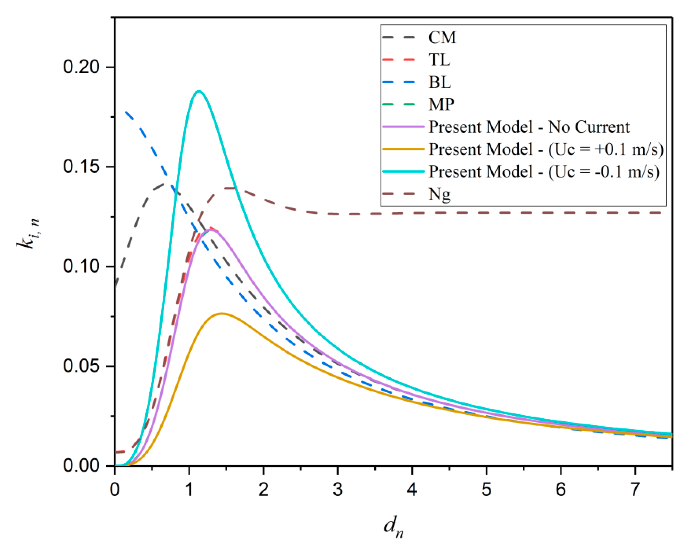
As shown by the literature studies, the dissipation rates versus dimensionless mud thickness, d_n shows a local peak around d_p=1.2, which is the dimensionless thickness with the maximum dissipation rate. Figure 2 presents the dissipation rate, k_i, plotted against the dimensionless mud thickness, d_n, for different models. TL, MP and the proposed models predict same values for the dissipation rate. The CM model provides different values with a trend similar to those of the other models especially for lower values of d_n. Note that the CM assumptions are appropriate for the cases where the fluid mud layer is deep, e.g., d_n is large (i.e., low depth, or high viscosity). Ng model shows the same local peak as that of the other models with an ascending phase followed by a constant phase by an increase in d_n. This is due to the assumption that the mud thickness is similar to its boundary layer thickness, so that the dissipation rate remains constant by further increasing the d_n. However, the BL model is not showing the local peak because this model is applicable to a mud layer of infinite depth. The counter-current provides higher values of the dissipation rate compared to the no current and co-current cases (Figure 2) because in the presence of counter-current, the wave length is decreased, while the wave height is increased.

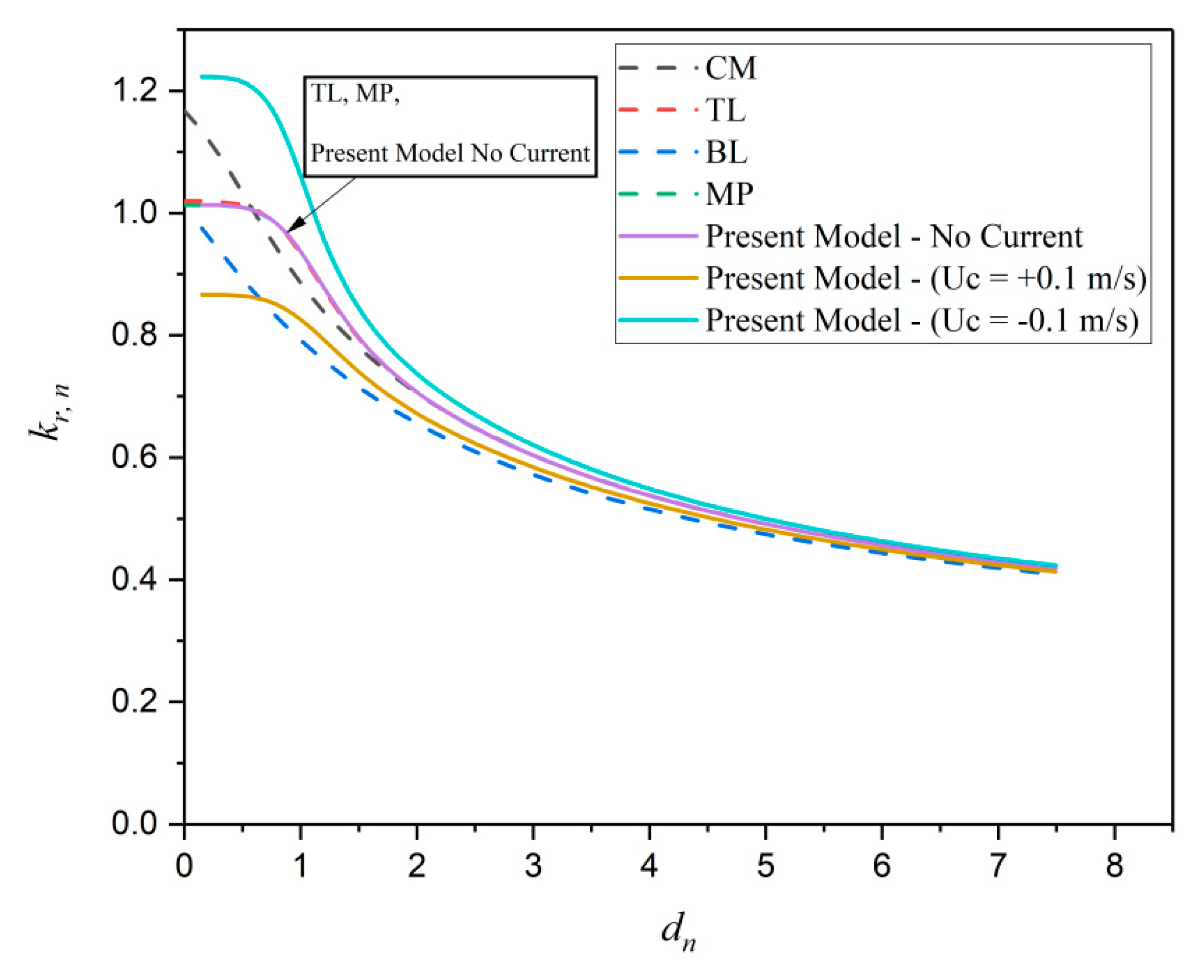
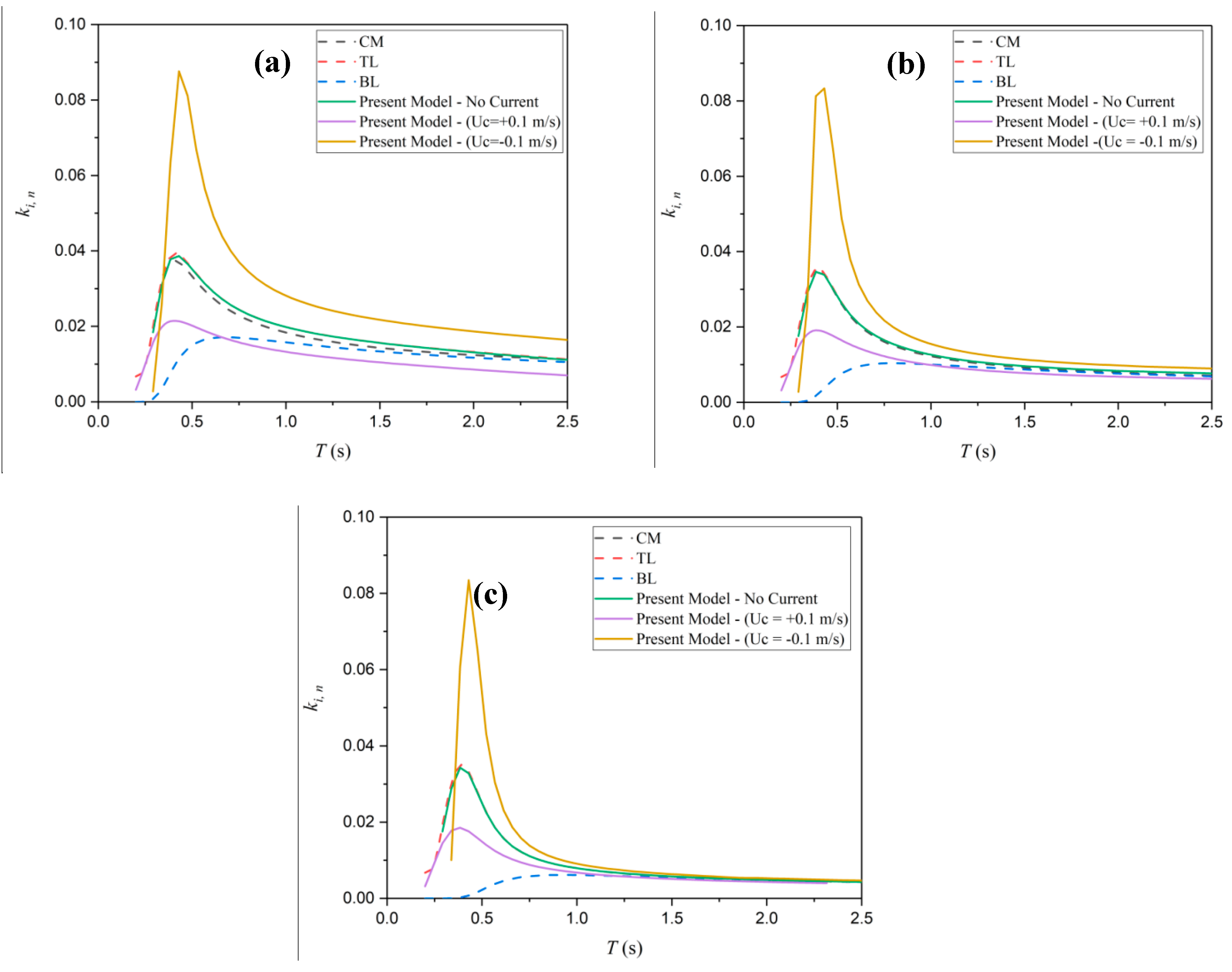
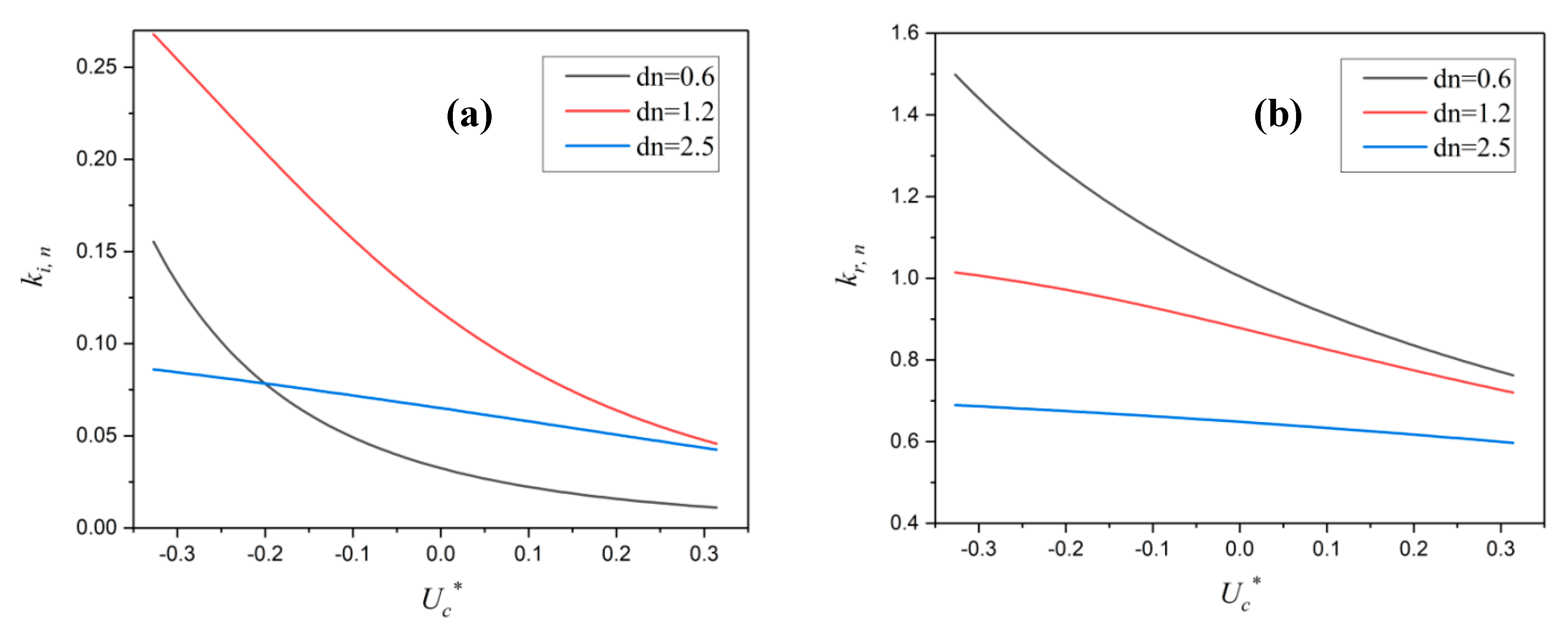
The wave number decreases as the dimensionless mud thickness increases (Figure 3). TL, MP, and the proposed model provide similar values for the wave number. CM and BL models show higher and lower values of the wave number at lower values of d_n, respectively. Figure 4 shows the dissipation rate versus wave period for three different mud thicknesses. While a local peak is provided by CM, TL, and proposed model, BL model does not show that peak. The BL model does not perform differently from the other models for larger values of mud thickness. The proposed model provides a sharp peak with a sharp ascending phase in the presence of counter current because its solutions are sensible to the initial values which makes the results to oscillate to the second mode (slow mode). Figure 5 shows the dissipation rate and wave number respectively which are plotted against the current velocity, ${U_c}^{*}$ for three different dimensionless mud thicknesses. Both wave dissipation rates and the wave number decrease as the velocity turns from negative values (counter-current) into positive values (co-current). The presence of co-current results in higher values of wave number and lower values of wave height.

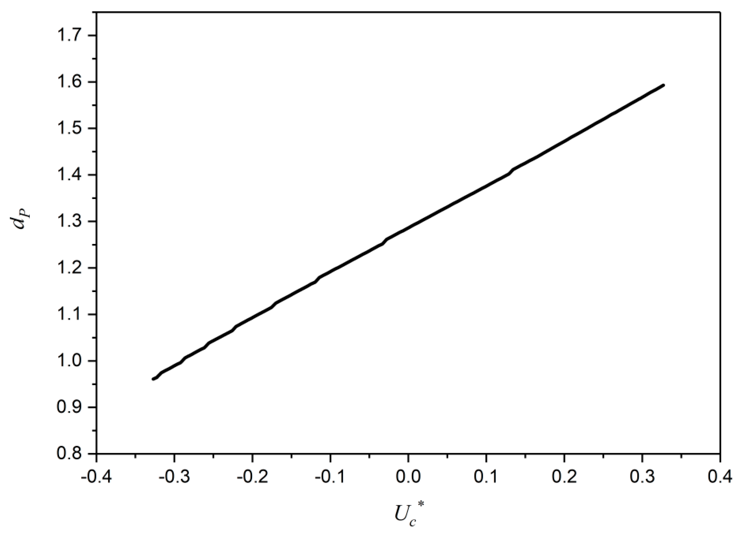
Figure 6 shows the peak values of the dimensionless mud thickness against the current velocity. The peak values of dimensionless mud thickness increases with an increase in the current velocity (i.e., moving from counter to co-current).

5.1.2. Comparison with the Laboratory Data

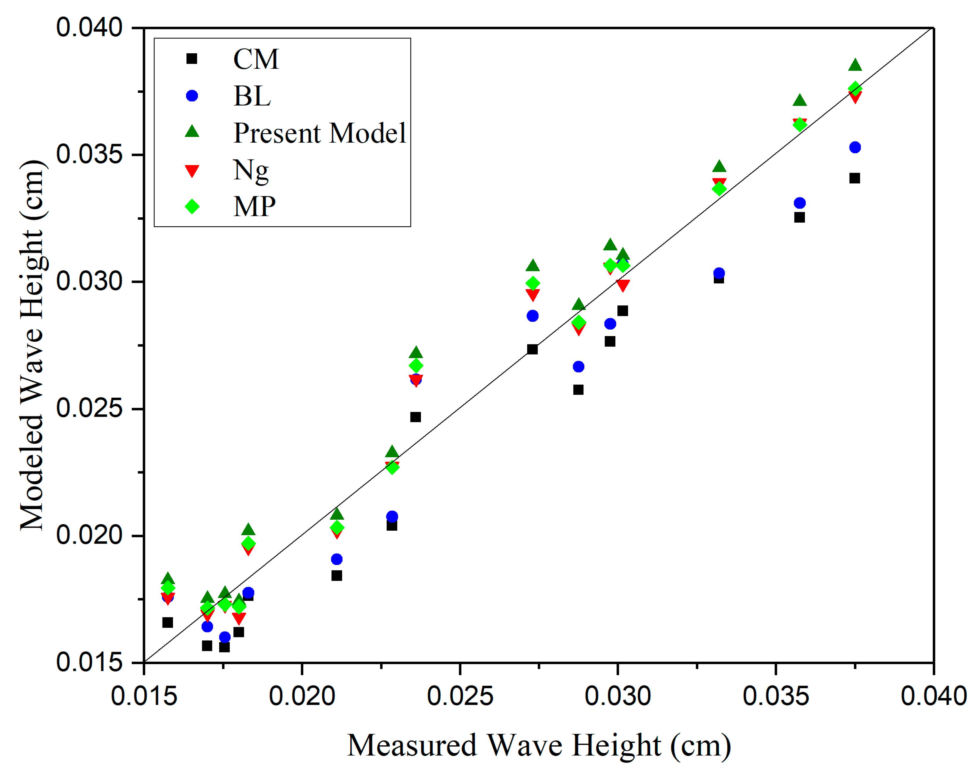
Figure 7 compares the modeled values of wave height with the experimental measurements corresponding to the gauge 2 and 4 in the laboratory experiments [11]. As expected, CM and BL models present poorer predictions compared to the other three models due to their assumptions of thick mud layer (or lower viscosities of mud) which do not match well the experimental set-up. The relative difference, presented in

Table A1. Comparison of laboratory data and model outputs of dissipated wave height for no current case.

Measured Wave Height (m)	CM		BL		Ng		Proposed Model
	Modeled Wave Height (m)	Relative Difference	Modeled Wave Height (m)	Relative Difference	Modeled Wave Height (m)	Relative Difference	Modeled Wave Height (m)	Relative Difference
0.0181	0.0162	−0.0414	0.0172	−0.0414	0.0168	−0.0663	0.0174	−0.0331
0.0301	0.0289	0.0199	0.0307	0.0189	0.0299	−0.0080	0.0310	0.0299
0.0172	0.0157	−0.0349	0.0164	−0.0348	0.0169	−0.004	0.0175	0.0291
0.0273	0.0273	0.0512	0.0287	0.0513	0.0295	0.0820	0.0306	0.1209
0.0211	0.0184	−0.0948	0.0191	−0.0948	0.0211	−0.0436	0.0208	−0.01422
0.0287	0.0257	−0.0697	0.0267	−0.0725	0.0282	−0.0188	0.0291	0.0104
0.0175	0.0156	−0.0857	0.0161	−0.0886	0.0173	-0.016	0.0177	0.0115
0.0357	0.0325	−0.0728	0.0331	−0.0739	0.0360	0.0146	0.0371	0.0364
0.0157	0.0166	0.1146	0.0176	0.1172	0.0176	0.1172	0.0183	0.1592
0.0236	0.0247	0.1089	0.0262	0.1089	0.0262	0.1089	0.0272	0.1525
0.0273	0.0273	0.0498	0.0287	0.0498	0.0295	0.0820	0.0306	0.1209
0.0375	0.0341	−0.0586	0.0353	−0.0587	0.0373	−0.0043	0.0385	0.0267
0.0297	0.0276	−0.0471	0.0283	−0.0471	0.0306	0.0269	0.0314	0.0572
0.0228	0.0204	−0.0921	0.0208	−0.0020	0.0227	-0.0001	0.0233	0.0004
0.0183	0.0176	−0.0290	0.0178	−0.0005	0.0195	0.0012	0.0202	0.0019
0.0332	0.0301	−0.0858	0.0303	−0.0028	0.0339	0.0007	0.0345	0.0013

(Appendix C), quantifies the poorer predictions of the mentioned models in comparison with the other models. The BL model generally underpredicts small and large values of the attenuated wave height. This might be related to the BL assumptions corresponding to the deep mud layers with low viscosity.

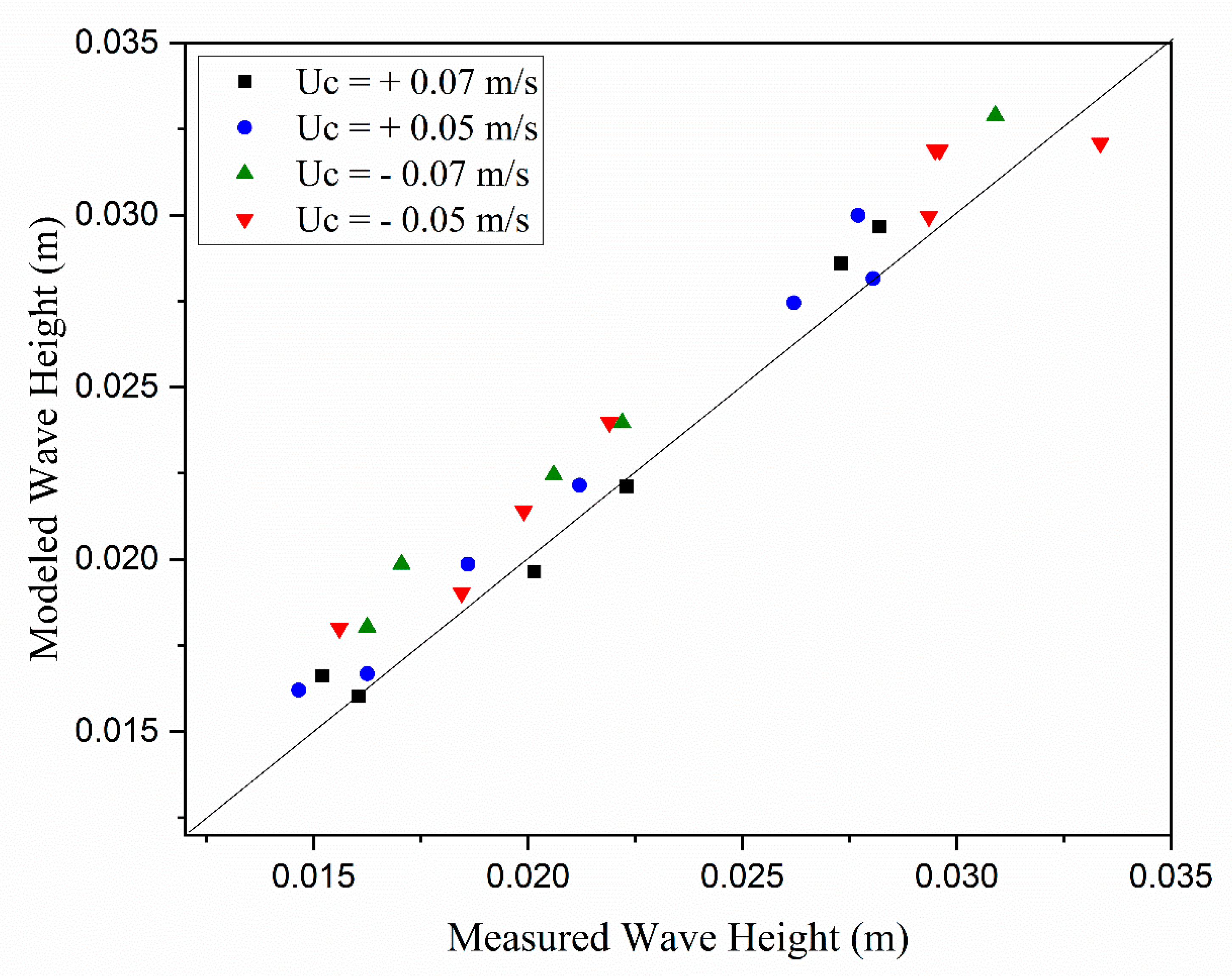
Figure 8 provides a comparison of measured and modeled attenuated wave height for the co- and counter-current cases. The proposed model provides predictions close to the measurements for the co-current cases and the larger current values (e.g., $U_c$ = 0.07 m/s). This is because, the wave height is increased in the counter currents for which the small amplitude linear wave theory, applied in this study, might not be valid any more. Table A1 in the Appendix C lists the values of the measured and modeled dissipated wave heights. The relative difference between the model and the experimental results was calculated with Equation 95.

Table A2. Comparison of laboratory data and proposed model outputs of dissipated wave height for co- and counter current cases. LD means Laboratoray Data; PM means Proposed Model; RD means Relative Difference.

Uc = +0.07 m/s			Uc = −0.07 m/s			Uc = +0.05 m/s			Uc= −0.05 m/s
Wave Height (m)		RD	Wave Height (m)		RD	Wave Height (m)		RD	Wave Height (m)		RD
LD	PM		LD	PM		LD	PM		LD	PM
0.01605	0.0161	0	0.0170	0.0199	0.1647	0.0162	0.0170	0.0247	0.0184	0.0194	0.0326
0.0273	0.0286	0.0476	0.0162	0.0183	0.1111	0.0280	0.0281	0.0036	0.0333	0.0321	–0.0300
0.0152	0.0166	0.0921	0.0206	0.0224	0.0874	0.0146	0.0162	0.1096	0.0156	0.0180	0.1538
0.0201	0.0196	–0.0249	0.0309	0.0329	0.0647	0.0186	0.0199	0.0699	0.0199	0.0214	0.0754
0.0282	0.0297	0.0531	0.0222	0.0242	0.0811	0.0277	0.0302	0.0830	0.0295	0.0324	0.0813
0.0223	0.0221	–0.0089	0.0309	0.0329	0.0647	0.0212	0.0222	0.0424	0.0219	0.0243	0.0959
0.0282	0.0297	0.0532	-	-	-	0.0262	0.0274	0.0458	0.0296	0.0321	0.0777
-	-	-	-	-	-	-	-	-	0.0293	0.0300	0.0205

of Appendix C presents the same results for the co-current and counter-current cases showing that the relative differences are quite small (lower than O (0.001 m)).

$$\mathrm{Relative}\mathrm{difference}=\left(\mathrm{Model}\mathrm{outputs}-\mathrm{Experimental}\mathrm{results}\right)/\mathrm{Experimental}\mathrm{results}.$$

(95)

5.2. Velocity Amplitude

5.2.1. Model Outputs

Figure 9 shows the water velocity amplitudes against the dimensionless mud thickness. The velocity amplitude increases as the dimensionless mud thickness increases. All models, except BL and Ng, show that the velocity amplitude is unchanged for small values of d_n. However, BL and CM models show a descending trend for all values of d_n. This is due to the assumption of BL and CM models (e.g., deeper lower layer) differing from those of the other models, which might not be applicable for small values of d_n, i.e., the high mud viscosity applied in this study. The variation of mud particles velocity against the dimensionless mud thickness is plotted in Figure 10. The results from the Ng model are one order of magnitude smaller than those from the other models for large values of mud thickness because Ng [5] assumed that the mud thickness is of the same order as the mud boundary layer thickness (i.e., d_n = O [1]). Thus, the results are not applicable to the large values of d_n. The BL model shows a drop for intermediate d_n. This might be due to a shift between the boundary layer solution and potential flows for small and large values of d_n, respectively.

5.2.2. Comparison with the Laboratory Data

Figure 11 presents a comparison between the model outputs of the velocity profiles and the measurements. The results from BL model, corresponding to the velocity close to the rigid bottom, $U_3$, and Ng model were comparatively closer to the laboratory data than those from the other models. This could be explained with the highly viscous fluid mud used in the experiments with the thickness being of the same order as the boundary layer thickness. Thus, the boundary layer solution provided predictions closer to the experimental data. The other two solutions relevant to BL made flaws due to the small value of d_n in this case. The other models underpredict the results for the mud particles velocity. All models are in agreement with the measured values for the velocity in the water layer. The proposed model is in agreement with the laboratory data for the velocity profile in the mud layer in the case of co/counter current (Figure 11b,c). However, the model provides a better agreement for the co-current case. This is due to the nonlinear wave effects induced by the higher wave heights in the counter-current case.

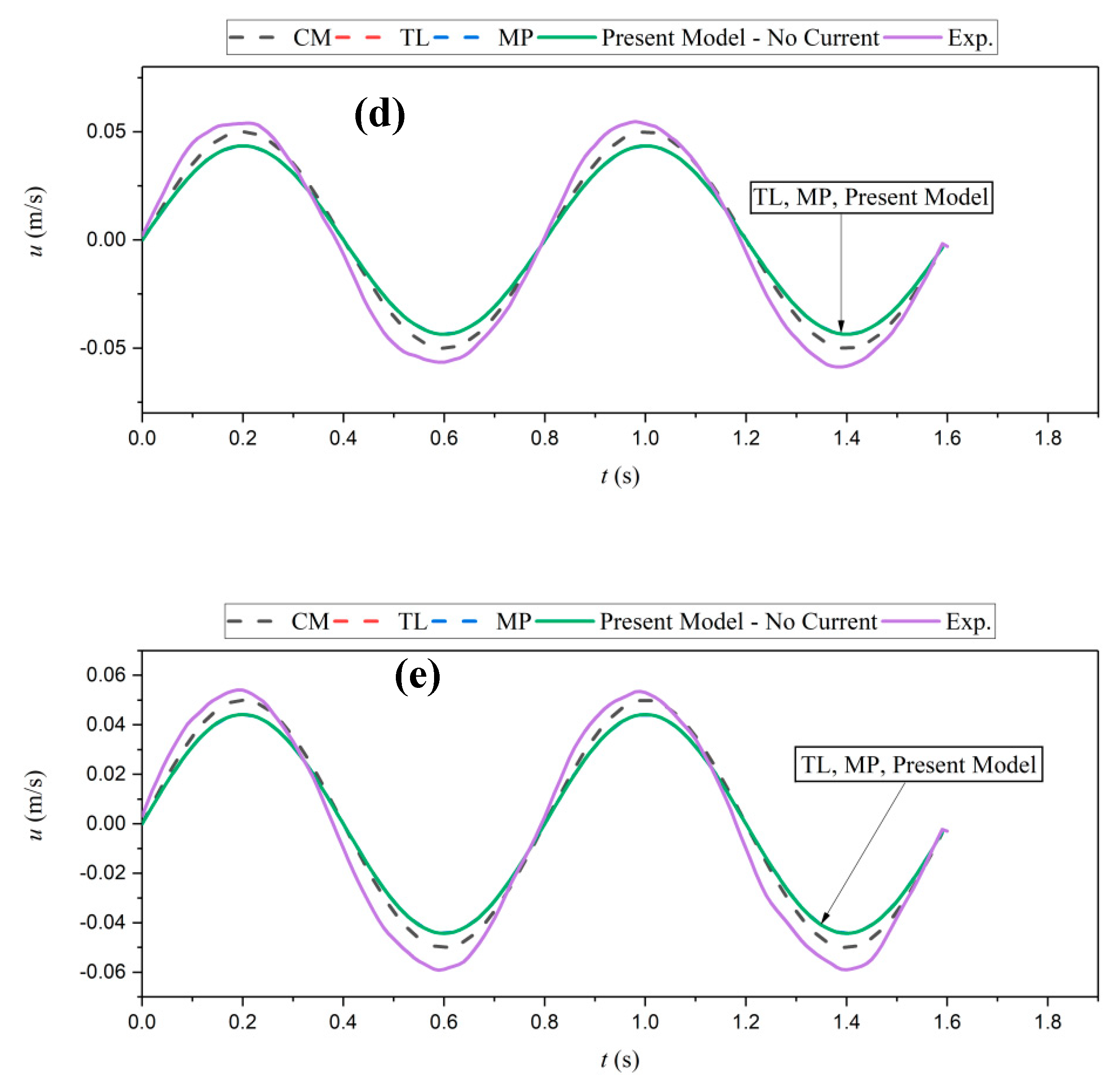
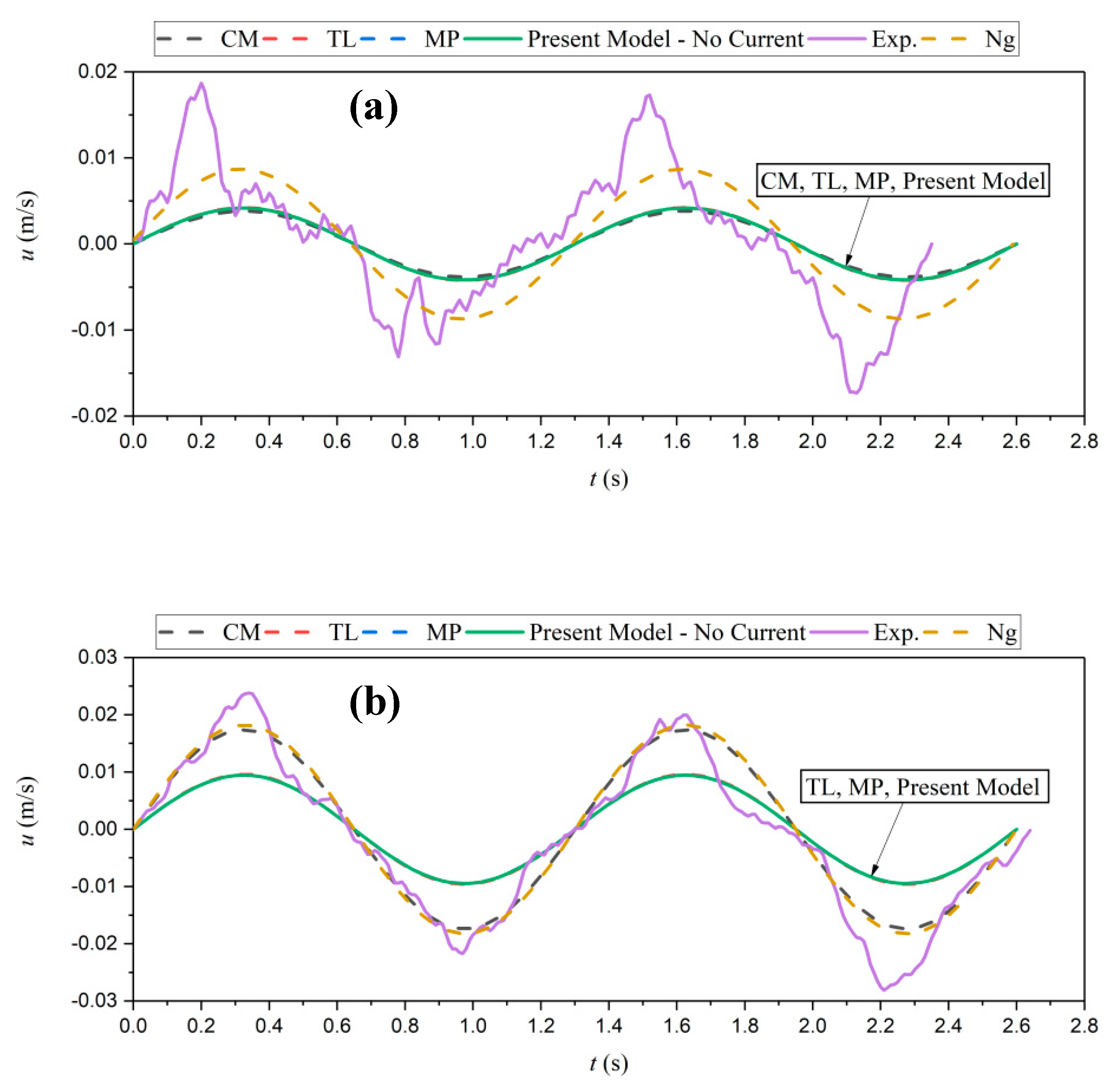
Figure 12 and Figure 13 present the time series of velocity for two representative cases, for five different depths of water and mud layers. Agreement with the measurements is achieved for the velocity in the water layer. However, the predictions are much closer to the experimental data in the case of higher water content ratio, W = 160% (i.e., lower viscosity, Figure 13d,e), especially those from the Ng model. This is because at higher values of viscosities, non-linear properties become more dominant and the Newtonian viscous models are not capable of accurately predicting the velocity. This is also true for the velocity in the mud layer (Figure 13; Figure 14a–c). The Ng model provides better results if compared to the proposed model, TL and MP models in the middle and upper parts of the mud layer (Figure 13b,c). However, in the lower parts of the mud layer, TL, MP, and the present model provide results closer to the measurements compared to the CM and Ng models. Such overprediction of Ng and CM is related to the boundary layer assumptions (applied by Ng) and considering the effect of viscosity close to the rigid bottom and interface (applied by CM). As observed in the figure, the experimental results are much more sensitive to the variation of z compared to the model outputs which are less sensitive to depth variations. Such sensitivity might be relevant to the vertical variations of the mud properties in the experiments. Some fluctuations are also observed in the experimental results, which were related to mud non-linearities and inhomogeneous mud properties.

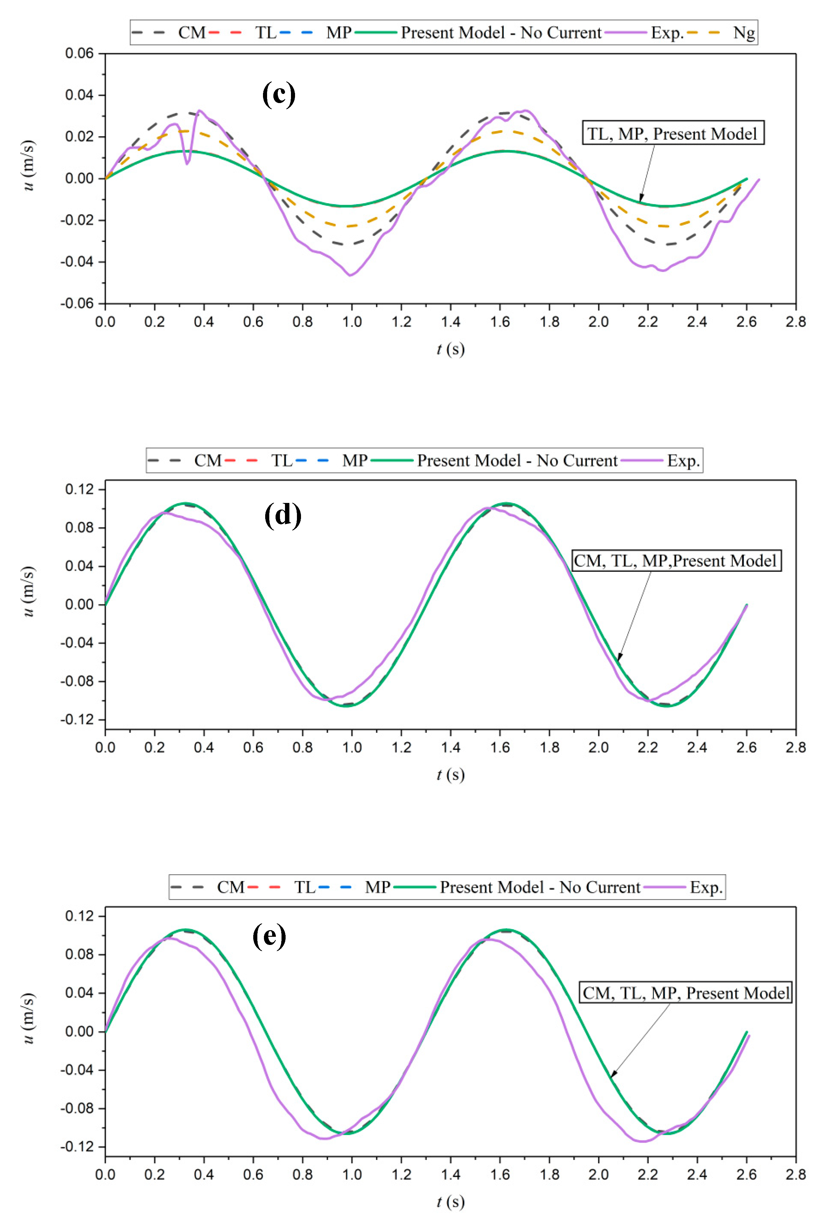
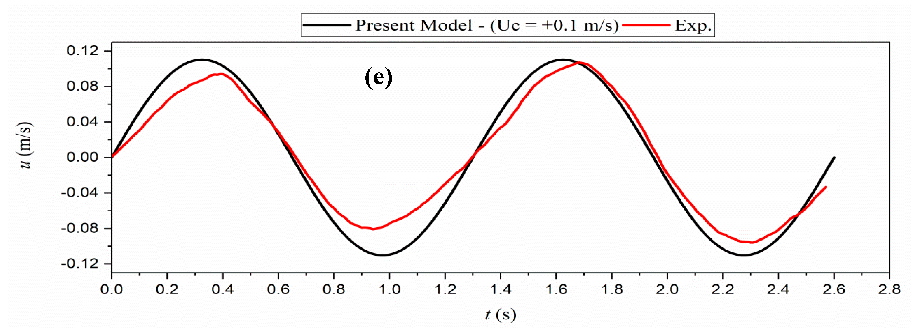
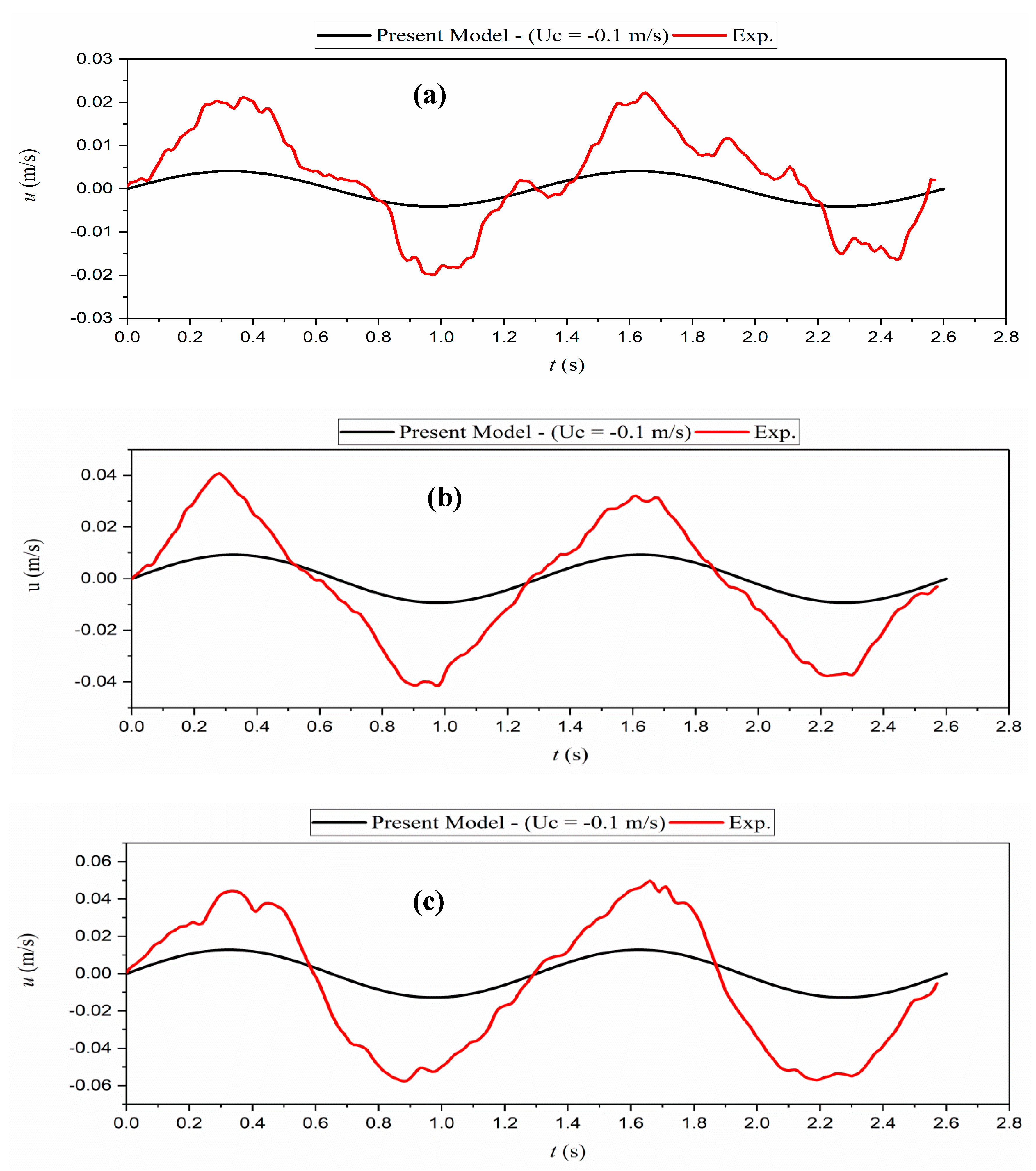
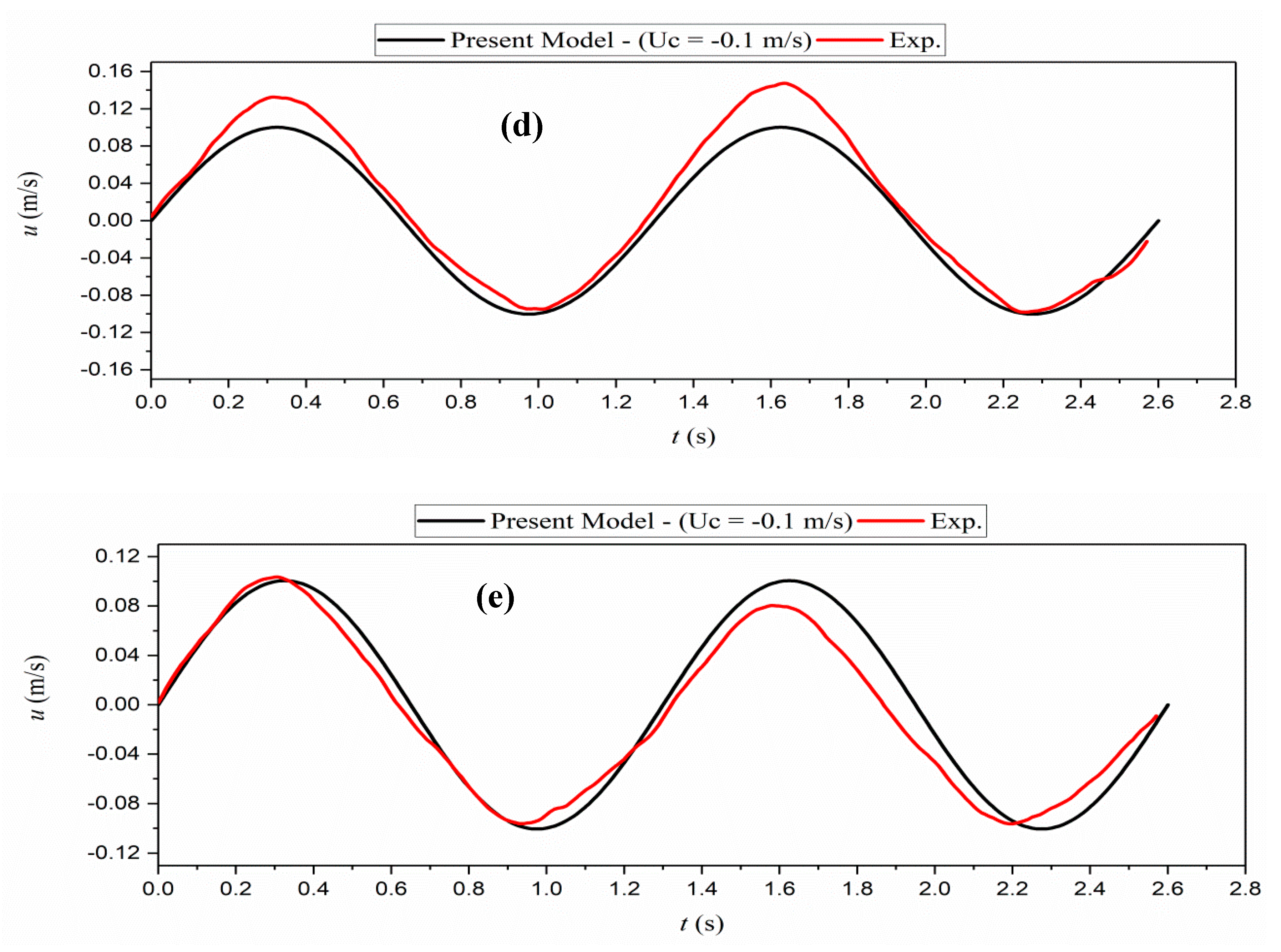
Figure 14 and Figure 15 present the time series of the velocity in the water and mud layers for the co-current ($U_c$= 0.1 m/s), and counter-current ($U_c$ = −0.1 m/s), respectively. The model is in agreement with the experimental data of water velocity in both cases. The proposed model underpredicts the velocity in the mud layer due to the application of the thin lower layer assumptions (TL). The model considers both the boundary layer effects and the wave effects, while the mud is assumed as a thin layer which leads to some underestimation of the velocity. Also, going deeper inside the mud layer (e.g., shifting from Figure 14 and Figure 15c to Figure 14 and Figure 15a), a higher discrepancy between the model outputs and the laboratory data was observed due to inhomogeneities through the mud depth induced by the gravity forces and the rigid bottom boundary layer effects.

5.3. Mass Transport

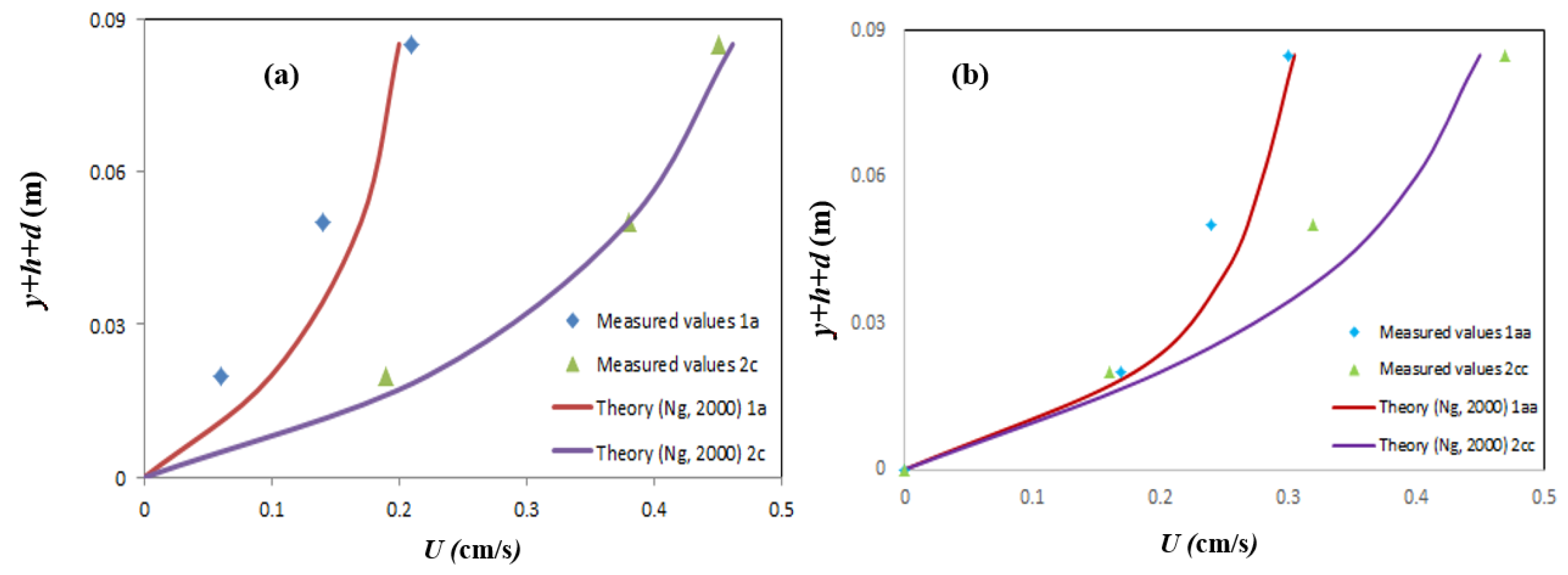
Figure 16 presents comparisons of the measured mass transport velocity and the analytical results of the model of Ng [5]. Figure 16a,b show that as the wave height increased, the mud mass transport velocity increased. The mass transport velocity is an order of magnitude smaller O (0.005 m/s) compared to the particle velocities, which are of O (0.05 m/s).

6. Conclusions

The literature models investigating the interactions between waves and mud were reviewed. The results of the models for the dissipation rate, wave number, and particle velocities were analyzed. The models outputs were also compared with the available laboratory data of experiments of Soltanpour et al. [11]. A new model in the case of wave-mud and wave–current–mud interactions was also proposed and its results were analyzed.

• The Ng model applies boundary layer assumptions for prediction of the dissipation rate and wave number, which results in different trends for higher values of dimensionless mud thickness. While CM and BL provide different results compared to the trend of other models for lower values of dimensionless mud thickness, i.e., the mentioned models provide constant values for wave number in lower values of dimensionless thickness.
• The Ng model and the present model show better agreement with the measurements in terms of the attenuated wave heights.
• The Ng model and the boundary layer solution of BL show better results for the velocity profiles close to the rigid bottom when compared to the laboratory data. The present model provides close predictions to the measurements for velocity amplitude profiles in the co-current case.
• All models successfully simulate the velocity time series; however, the Ng model provides predictions of velocity time series closer to the experimental data, especially in the case of higher water content ratio. Besides, none of the models is in agreement with the measurements for lower values of the water content ratio.

Further investigations considering other rheological models should be undertaken in future studies. It can be concluded that the Ng model provides closer results to the measurements in the prediction of particle velocities in the highly viscous mud layer.

The proposed model presents a straightforward dispersion relation considering the effects of co and counter-current in the case of thin mud layer. Such a straightforward solution of the wave number and the velocity coefficients in terms of the wave number allows the computation of the dissipation rate, particles velocity, and mass transport more rapidly while keeping the accuracy of the prediction in highly viscous mud layers. In terms of the attenuated wave heights, the proposed model was in better agreement with the experiments, in comparison to the results of BL and CM models. Similar to the MP and CM models, reasonable results of the profiles of particles velocities are obtained. Furthermore, the new model is also capable to simulate the wave height and particles velocities in the case of wave–current–mud interaction.

References

- Samsami, F.; Soltanpour, M.; Shibayama, T. Spectral analysis of irregular waves in wave–mud and wave–current–mud interactions. Ocean Dyn. 2015, 65, 1305–1320. [Google Scholar] [CrossRef]
- Gade, H.G. Effects of a nonrigid, impermeable bottom on plane surface waves in shallow water. J. Mar. Res. 1958, 16, 61–81. [Google Scholar]
- Dalrymple, R.A.; Liu, P.L.F. Waves over soft muds: a two-layer fluid model. J. Phys. Oceanogr. 1978, 8, 1121–1131. [Google Scholar] [CrossRef]
- Macpherson, H. The attenuation of water waves over a non-rigid bed. J. Fluid Mech. 1980, 97, 721–742. [Google Scholar] [CrossRef]
- Ng, C.-O. Water waves over a muddy bed: a two-layer Stokes’ boundary layer model. Coast. Eng. 2000, 40, 221–242. [Google Scholar] [CrossRef]
- Liu, P.L.-F.; Chan, I.-C. A note on the effects of a thin visco-elastic mud layer on small amplitude water-wave propagation. Coast. Eng. 2007, 54, 233–247. [Google Scholar] [CrossRef]
- Kranenburg, W.M.; Winterwerp, J.C.; de Boer, G.J.; Cornelisse, J.M.; Zijlema, M. SWAN-Mud: Engineering model for mud-induced wave damping. J. Hydraul. Eng. 2011, 137, 959–975. [Google Scholar] [CrossRef]
- Sakakiyama, T.; Byker, E.W. Mass transport velocity in mud layer due to progressive waves. J. Waterw. Port Coastal Ocean Eng. 1989, 115, 614–633. [Google Scholar] [CrossRef]
- An, N.N.; Shibayama, T. Wave-current interaction with mud bed. In Proceedings of the Coastal Engineering; ASCE: Reston, VA, USA, 1994; Volume 1, pp. 2913–2927. [Google Scholar]
- Hsu, W.Y.; Hwung, H.H.; Hsu, T.J.; Torres-Freyermuth, A.; Yang, R.Y. An experimental and numerical investigation on wave-mud interactions. J. Geophys. Res. Ocean. 2013, 118, 1126–1141. [Google Scholar] [CrossRef] [Green Version]
- Soltanpour, M.; Shamsnia, S.H.; Shibayama, T.; Nakamura, R. A study on mud particle velocities and mass transport in wave-current-mud interaction. Appl. Ocean Res. 2018, 78, 267–280. [Google Scholar] [CrossRef]
- Zhang, D.-H.; Ng, C.-O. A numerical study on wave-mud interaction. China Ocean Eng. 2006, 20, 383–394. [Google Scholar]
- Niu, X.; Yu, X. A numerical model for wave propagation over muddy slope. In Proceedings of the Coastal Engineering; ASCE: Reston, VA, USA, 2011; Volume 1, p. 27. [Google Scholar]
- Hejazi, K.; Soltanpour, M.; Sami, S. Numerical modeling of wave–mud interaction using projection method. Ocean Dyn. 2013, 63, 1093–1111. [Google Scholar] [CrossRef] [Green Version]
- Beyramzade, M.; Siadatmousavi, S.M. Implementation of viscoelastic mud-induced energy attenuation in the third-generation wave model, SWAN. Ocean Dyn. 2018, 68, 47–63. [Google Scholar] [CrossRef]
- Haghshenas, S.A.; Soltanpour, M. An analysis of wave dissipation at the Hendijan mud coast, the Persian Gulf. Ocean Dyn. 2011, 61, 217–232. [Google Scholar] [CrossRef]
- Nakano, S. Wave Damping and Mud Transport; Kyoto University: Kyoto, Japan, 1994. [Google Scholar]
- Siadatmousavi, S.M.; Allahdadi, M.N.; Chen, Q.; Jose, F.; Roberts, H.H. Simulation of wave damping during a cold front over the muddy Atchafalaya shelf. Cont. Shelf Res. 2012, 47, 165–177. [Google Scholar] [CrossRef]
- Papakonstantinou, J. The historical development of the secant method in 1-d. In Proceedings of the Annual Meeting of the Mathematical Association of America, San Jose, CA, USA, 3–5 August 2007. [Google Scholar]
- Soltanpour, M.; Shamsnia, H.; Shibayama, T.; Nakamura, R.; Tatekoji, A. A study on wave-induced particle velocities in fluid mud layer. In Proceedings of the Coastal Engineering; ASCE: Reston, VA, USA, 2017; Volume 1, p. 28. [Google Scholar]
Figure 1.
Sketch of the wave-mud interaction for different models; (Modified from Haghshenas and Soltanpour [16]).
Figure 2.
Dissipation rate versus mud dimensionless thickness.
Figure 3.
Wave number versus dimensionless mud thickness.
Figure 4.
Dissipation rate versus wave period, T for (a) dn=5; (b) dn=8; (c) dn=12.
Figure 5.
(a) Dissipation rate (b) wave number versus current velocity.
Figure 6.
Peak value of the dimensionless mud thickness versus the current velocity.
Figure 7.
Comparison between experimental data and modeled values of attenuated wave height for no current case.
Figure 8.
Comparison between measured and modeled values of attenuated wave height for counter and co-currents.
Figure 9.
Water velocity (y = −0.5h) versus dimensionless mud thickness, T = 1.4 s; h = 0.0381 m; νw = 0.0000026 m2/s; νm = 0.0026 m2/s; ρw = 859.3 kg/m3; ρm = 1504 kg/m3.
Figure 10.
Water velocity (y = −(h+0.5d) versus dimensionless mud thickness, T = 1.4 s; h = 0.0381 m; νw = 0.0000026 m2/s; νm = 0.0026 m2/s; ρw = 859.3 kg/m3; ρm = 1504 kg/m3.
Figure 11.
Comparison of velocity profiles of different analytical models and measurements, T = 1.1 s; H = 0.05 m; W = 160%; (a) no current, (b) Uc = 0.07 m/s, (c) Uc = −0.07 m/s.
Figure 12.
Time series of velocity for T=0.8 s, H=0.04 m, W=130%; (a) 0.02 m; (b) 0.05 m; (c) 0.085 m; (d) 0.12 m; (e) 0.135 m above the rigid bed.
Figure 13.
Time series of velocity for T = 1.3 s, H = 0.05 m, W = 160%; (a) 0.02 m; (b) 0.05 m; (c) 0.085 m; (d) 0.12 m; (e) 0.135 m above the rigid bed.
Figure 14.
Time series of velocity for T=1.3 s, H=0.05 m, Uc=0.1 m/s; W=160%; (a) 0.02 m; (b) 0.05 m; (c) 0.085 m; (d) 0.12 m; (e) 0.135 m above the rigid bed.
Figure 15.
Time series of velocity for T = 1.3 s, H = 0.05 m, Uc = −0.1 m/s; W = 160%; (a) 0.02 m; (b) 0.05 m; (c) 0.085 m; (d) 0.12 m; (e) 0.135 m above the rigid bed.
Figure 16.
Comparisons between the measured mass transport rates and analytical model of Ng (2000), (a) H = 0.04 m, and T = 1.0 s (1a); H = 0.07 m, T = 1.1 s (2c); (b) H = 0.07 m, T = 1.2 s (1aa); H = 0.08 m, T = 1.3 s (2cc).