Article

Impact of Nonzero Intercept Gas Transfer Velocity Parameterizations on Global and Regional Ocean–Atmosphere CO2 Fluxes

by
Mariana Ribas-Ribas
1,*,
Gianna Battaglia
2,
Matthew P. Humphreys
3 and
Oliver Wurl
1
1
Center for Marine Sensors, Institute for Chemistry and Biology of the Marine Environment, Carl von Ossietzky University Oldenburg, 26129 Wilhelmshaven, Germany
2
Climate and Environmental Physics, Physics Institute, and Oeschger Centre for Climate Change Research, University of Bern, 3012 Bern, Switzerland
3
Centre for Ocean and Atmospheric Sciences, School of Environmental Sciences, University of East Anglia, Norwich NR4 7TJ, UK
*
Author to whom correspondence should be addressed.
Geosciences 2019, 9(5), 230; https://doi.org/10.3390/geosciences9050230
Submission received: 15 March 2019 / Revised: 6 May 2019 / Accepted: 13 May 2019 / Published: 20 May 2019
(This article belongs to the Special Issue Ocean-Atmosphere Interaction)

Abstract

:
Carbon dioxide (CO2) fluxes between the ocean and atmosphere (FCO2) are commonly computed from differences between their partial pressures of CO2pCO2) and the gas transfer velocity (k). Commonly used wind-based parameterizations for k imply a zero intercept, although in situ field data below 4 m s−1 are scarce. Considering a global average wind speed over the ocean of 6.6 m s−1, a nonzero intercept might have a significant impact on global FCO2. Here, we present a database of 245 in situ measurements of k obtained with the floating chamber technique (Sniffle), 190 of which have wind speeds lower than 4 m s−1. A quadratic parameterization with wind speed and a nonzero intercept resulted in the best fit for k. We further tested FCO2 calculated with a different parameterization with a complementary pCO2 observation-based product. Furthermore, we ran a simulation in a well-tested ocean model of intermediate complexity to test the implications of different gas transfer velocity parameterizations for the natural carbon cycle. The global ocean observation-based analysis suggests that ignoring a nonzero intercept results in an ocean-sink increase of 0.73 Gt C yr−1. This corresponds to a 28% higher uptake of CO2 compared with the flux calculated from a parameterization with a nonzero intercept. The differences in FCO2 were higher in the case of low wind conditions and large ΔpCO2 between the ocean and atmosphere. Such conditions occur frequently in the Tropics.

1. Introduction

The Earth’s ocean currently absorbs about 26% of all anthropogenic carbon emissions, with an anthropogenic flux of ca. 2.4 Gt C yr−1 [1]. The ocean is a huge reservoir of CO2, and a better understanding of how the ocean absorbs CO2 is critical for predicting climate change. Carbon dioxide fluxes (FCO2) between the ocean and atmosphere are normally calculated from the difference between oceanic and atmospheric partial pressure of CO2 (pCO2) and gas transfer velocity (k):
FCO2 = kα ΔpCO2,
where α is the solubility depending on temperature and salinity [2].
The k is typically calculated from parameterizations depending solely on wind speed, as reviewed by Wanninkhof [3]. However, these parameterizations lack in situ data for the low wind regimes, that is, wind speed <4 m s−1 [4]. Therefore, they assume that for wind speed close to zero, the k is also zero.
The nonzero intercept is important for CO2 budgets inferred from ocean pCO2-based products, because there are large oceanic regions with prevailing low wind conditions (in Archer and Jacobson [5] and in Wurl, et al. [6]) (e.g., the Mediterranean Sea in summer and the tropical Pacific). Low wind regimes with limited surface mixing can lead to stratification of the upper layer and, given favorable conditions and assuming the nutrients are not limiting, to increased ocean productivity that would decrease the pCO2 in the surface ocean and would increase the ΔpCO2. With commonly used k parameterizations, these regions will have a net FCO2 close to zero during periods of low sea states because the parameterization will predict k to be equal or close to zero. Consequently, the ocean’s source will be underestimated in low wind regime regions, such as the Tropical Ocean. It is important to quantify the associated bias as ocean pCO2-based flux products offer one approach to estimating the global uptake of anthropogenic carbon [1,7,8].
Parameterizations with a nonzero intercept have been reported in [9,10,11,12,13,14,15], and the nonzero intercept ranges from 1 to 15 cm h−1. Gas transfer velocity is unlikely to approach zero during low wind conditions as the wind speed is not the only main factor driving gas transfer across the surface; surface currents, buoyancy fluxes, micro breaking waves, and the presence of surface films (i.e., sea surface microlayer) affect gas transfer as well [3].
Zhang and Cai [16] reported potential biases based on an assumed nonzero intercept of 10 cm h−1 reported in published papers [10,17,18,19] and pointed out that if such a nonzero intercept is adapted, the global CO2 uptake for the year 1995 would increase by 0.2 Gt C yr−1. However, they also pointed out that more in situ data are required to compute nonzero intercepts and to combine model and observational studies in order to draw more robust conclusions about relevant cases.
The purpose of this study is to quantify the uncertainty of global and regional carbon fluxes introduced by uncertain gas transfer velocity parameterizations. We first present empirical evidence for a nonzero intercept in gas transfer velocity parameterizations by presenting a database of 245 in situ measurements of FCO2. We then use this database to evaluate the influence of the nonzero intercept on flux calculations. Hence, the evaluation of these parameterizations should not be seen as a way to promote our new parameterization as we and others have already determined that wind speed is not the only force that determines gas transfer velocities [9,20,21,22] and have identified other parameters, such as turbulent kinetic energy and surfactants, that affect the transfer. We believe the analysis offered by this paper is important because wind-based parameterizations are the most commonly used parameterizations, and because wind speed is an easier parameter to measure and/or is available from different sources. For these reasons, we evaluate the impact of the flux with and without an intercept on the gas transfer velocity parameterization and quantify the differences, that is, by assuming the flux is close to zero when wind speeds are close to zero. In a second step, we quantify the impact of nonzero intercept parameterizations on estimates of the oceanic uptake of carbon using a global pCO2-based product. To calculate differences in global and regional FCO2, five different gas transfer velocity parameterizations were used with the global maps of pCO2 spanning 1982–2018; two commonly used parameterizations had a zero intercept, and three parameterizations included a nonzero intercept. In a third step, we tested the implications of a nonzero intercept in the framework of a global three-dimensional ocean carbon cycle model. We discuss the short-term and long-term evolution of the FCO2 and the evolution of the natural carbon inventories in the ocean and atmosphere after introducing a nonzero intercept. We present both the global evolution of these variables and spatial patterns of change. The model is run for 5000 years, such that the system has time to approach new steady state conditions.

2. Materials and Methods

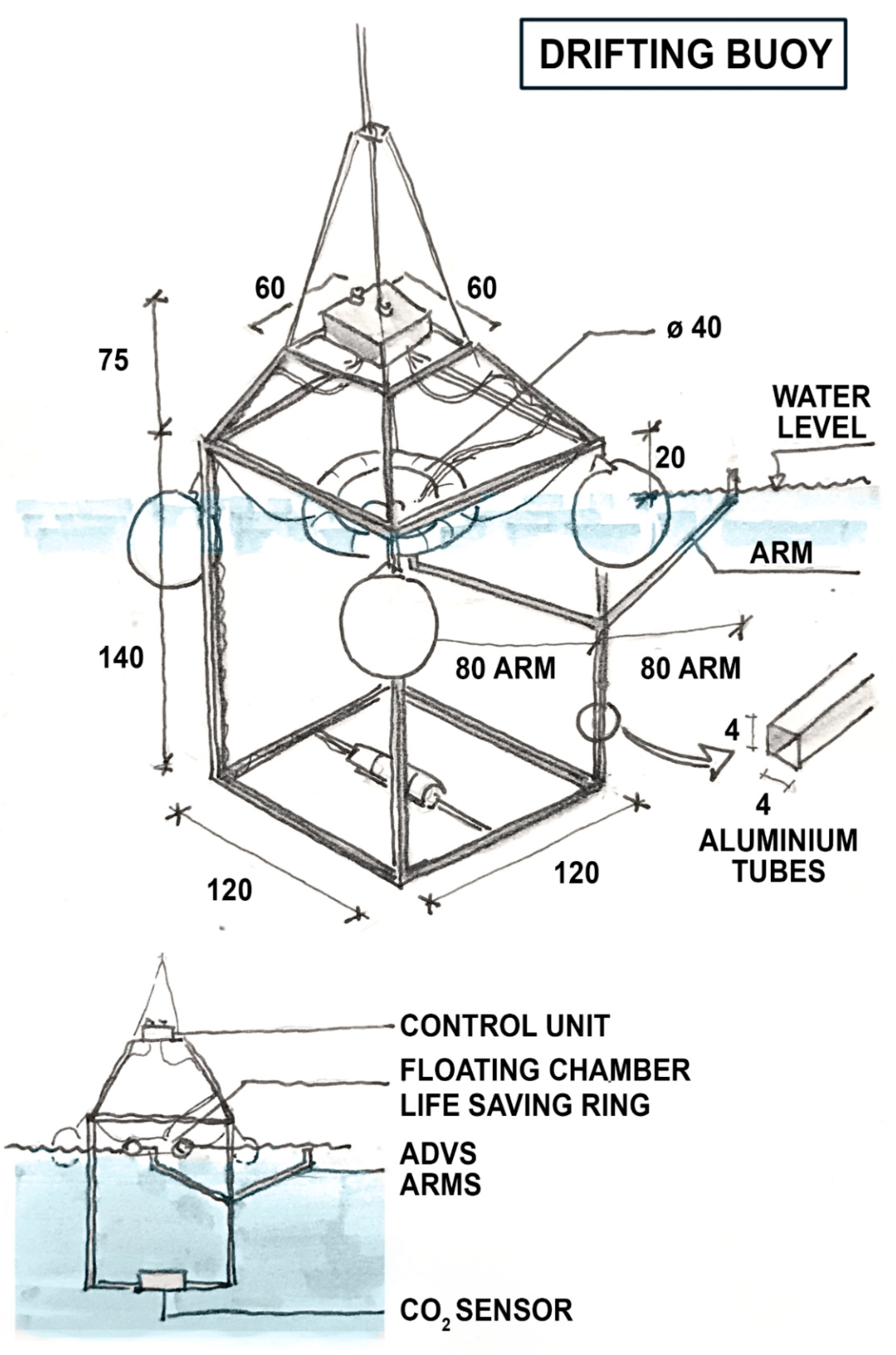
2.1. In Situ Flux Measurements with the Sniffle Floating Chamber

The field measurements were performed during several cruises (Table 1). An autonomous drifting buoy, Sniffle, was deployed to measure the partial pressure of CO2 (pCO2) in the air, at a water depth of 1.2 m, and inside a floating chamber. The Sniffle is described in detail in Ribas-Ribas, et al. [23] and a diagram is presented in Figure 1.
In short, we used the floating chamber technique and measured the turbulence inside and outside the chamber simultaneously to see if turbulence affected the measurements. Furthermore, we monitored temperature, humidity, and pressure inside the floating chamber in order to detect any problems in the measurements. This procedure allowed us to overcome the problems associated with floating chamber techniques identified by previous research. Using this approach, we were able to measure the short temporal and spatial resolution needed to understand the rapid gas transfer velocity processes, in contrast to other techniques, such as eddy covariance or dual tracers. pCO2 was determined using an infrared gas analyzer (OceanPack LI-COR LI-840X; SubCtech GmbH, Germany). The salinity, temperature, and wind speed were obtained from the research catamaran S3 [24] deployed simultaneously with the Sniffle. The CO2 fluxes were calculated as follows:
F CO 2 = dpCO 2 dt   V S   T   R ,
where d p C O 2 d t is the slope of the pCO2 change in the floating chamber, V is the volume of the floating chamber, S represents the surface area of the floating chamber, T represents the water temperature at a depth of 1 m from S3, and R is the gas constant. Measurements were excluded when the regression for the slope of the pCO2 change in the floating chamber was R² < 0.90. The equation of the gas transfer velocity k w is
k w = F CO 2 α   ( pCO 2   water pCO 2   air )
The solubility coefficient α depends on the temperature and salinity of the seawater and was calculated according to Weiss [2]. Finally, k w was standardized to k with the following formula:
k = k w ( 660 Sc ) 0.5 ,
S c is the temperature-dependent Schmidt number Wanninkhof [3]. More details about the gas transfer velocities and CO2 data from some of the cruises can be found in Mustaffa, et al. [9], Banko-Kubis, et al. [20], Ribas-Ribas, et al. [23], Stolle, et al. [25].
As a further quality control analysis for the floating chamber technique, we only used data with wind speeds lower than 7 m s−1 (to avoid breaking-wave interference with the chamber), and we deleted outliers, defined as more than three standard deviations from the mean in each wind bin (2.4% of our data). A least squares quadratic regression with wind speed was used to determine the nonzero intercept parameterization that best represented the flux measurements. This new parameterization was compared with the zero intercept parameterization of Wanninkhof [3]. We used the ancillary data measured during the measurement campaigns detailed in Table 1. Accurate uncertainty estimations are difficult. Therefore, we assumed a maximum uncertainty of 10% for all parameters (worst scenario) (i.e., volume and surface of floating chamber, temperature and salinity, and pCO2) affecting the calculation of k, as done before in [26] and [23]. We then propagated these errors on our calculations according to the method used by Taylor [27], resulting in 10.8% variation for CO2 fluxes [23].

2.2. Global Surface Ocean pCO2-Based Flux Product

We downloaded seawater and atmospheric pCO2 from http://www.bgc-jena.mpg.de/CarboScope/?ID=oc to calculate ΔpCO2. The pCO2 observation-based product was obtained by fitting a simple data-driven diagnostic model of ocean mixed-layer biogeochemistry [28] to surface-ocean CO2 partial pressure data from the Surface Ocean CO2 Atlas (SOCAT) [29]. Auxiliary datasets for sea surface salinity were taken from the World Ocean Atlas 2013 v2 https://www.nodc.noaa.gov/OC5/woa13/ (climatological mean field without temporal variability). We obtained data on wind speed and sea surface temperature with six-hourly temporal resolution from the ERA-Interim data product [30], which is produced by the European Centre for Medium-Range Weather Forecasts (https://www.ecmwf.int/en/forecasts/datasets/archive-datasets/reanalysis-datasets/era-interim). We then interpolated ΔpCO2 and salinity on the ERA-Interim grid. We carried out the FCO2 calculation in MATLAB (MathWorks) from wind speed, sea surface temperature, salinity, and ΔpCO2 at each ERA-Interim grid point using the “CO2flux” function available from https://github.com/mvdh7/co2flux. We then normalized each grid point from Rödenbeck, et al. [31] dataset by ocean surface area. Finally, we integrated FCO2 both globally and across each region of interest. We tested for five different parameterizations, as shown in Table 2.
Numerous parameterizations have been developed and reported, and we selected these five parametrizations for the two reasons: (i) The W is an update of a quadratic parameterization [33], commonly used since 1993 to estimate FCO2. K has a shorter history and has not been used as commonly as other parameterizations, but it is implemented in the Bern3D model used in our study. K is an extensive data-assimilation effort based on 14C isotopes. We then added the nonzero intercept to these two commonly used parametrizations (W+I and K+I) to evaluate the direct difference on adding the intercept. Finally, we evaluate the parametrization obtained from this study. (ii) Computing time is expensive, which limited us to investigating only five parameterizations.

2.3. Bern3D Ocean Model

The Bern3D Ocean Model of Intermediate Complexity is a three-dimensional frictional geostrophic ocean model [34] with an isopycnal diffusion scheme and Gent–McWilliams parameterization for eddy-induced transport [35]. It is coupled to a sea ice component, a single-layer energy moisture balance model of the atmosphere [36], a prognostic marine biogeochemistry module [37,38], and a sediment module [37]. The horizontal resolution is 41 by 40 grid cells, and there are 32 logarithmically scaled vertical layers. All model components share the same horizontal resolution. A monthly wind stress climatology [39] is prescribed at the surface. Model evaluation is presented in [40,41,42].
Ocean-atmosphere gas exchange and carbonate chemistry were modeled based on the Ocean-Carbon Cycle Model Intercomparison Project (OCMIP)-2 protocols [43,44], with updates for the calculation of the Schmidt number [3] and carbonate chemistry [45]. The gas transfer was computed according to Equation (5). In contrast with the OCMIP-2 protocols, the gas transfer velocity k in Bern3D scales increases linearly with wind speed, following [32], and the global mean ocean-atmosphere transfer rate is reduced by 19% compared with OCMIP-2 to match observation-based estimates of natural and bomb-produced radiocarbon [46]. The k (in m s−1 as implemented in the model) is therefore
k = 0.81 ( 1 F i c e ) 7.798 10 6 w i n d ( Sc 660 ) 0.5 ,
where Fice is the modeled sea ice concentration, wind is the prescribed climatology of monthly mean absolute wind speeds, and Sc is the Schmidt number following [3]. The normalization factor ensures the conservation of the globally integrated rate of annual mean gas transfer with respect to the original OCMIP formulation.
In a sensitivity experiment, a nonzero intercept is added to the gas transfer velocity function of CO2, such that
k K + I = k K + 3.06 10 5 [ m   s 1 ] ,
or, to unify with units
k K + I = k K + 11 [ cm   h 1 ] ,
Simulations start from preindustrial boundary conditions (A.D. 1765) with pCO2 prescribed at 278 ppm; model drift is negligible. The nonzero intercept is added to the k at every grid cell starting from the beginning of a run, after which CO2 is allowed to evolve freely. The simulation is run for 5000 years and changes in CO2 feedback on simulated climate.

3. Results

3.1. Flux Measurements with Sniffle

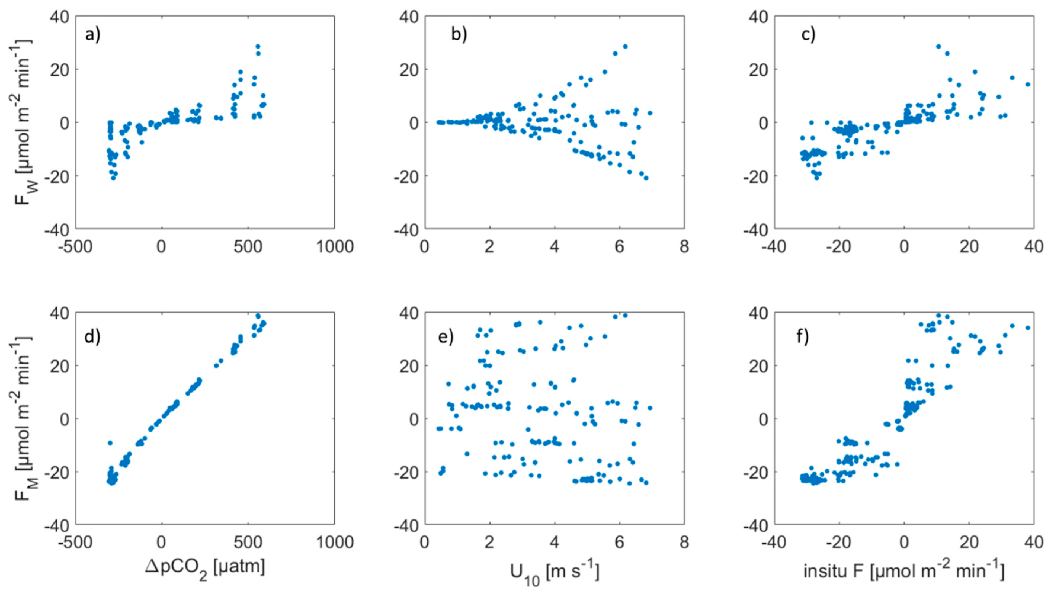
3.1.1. Parameterization

Figure 2 shows a mean value of the gas transfer velocity calculated from Sniffle of each binned wind speed normalized at 10 m and the wind speed distribution during six expeditions (see Table 1). Gas transfer velocities generally increased with wind speed. The data show the usual scatter from field measurements (see, for example, Johnson [4]). The excluded outliers did not arise from measurement technique problems (as we did a first-step quality control analysis to detect lifting of chamber and error in measurements inside the chamber). The outliers were probably real data (but mathematically outliers) due to biogeochemistry or physics factors, such as chemical enhancements, water or air side convection, and turbulence. During the measurement campaigns, we encountered wind speeds in a range from 0.4 to 10.5 m s−1, although we only used k values in which wind speed was lower than 7 m s−1 to avoid data with breaking waves in the chamber. At low wind speeds (U10 ≤ 4 m s−1), the k values varied between 0.5 and 14.6 cm h−1. At higher wind speeds (U10 > 4 but ≤7 m s−1), the k values varied between 0.9 and 32.8 cm h−1. The black line is the model that best fits the field data, and it is k660 = 5.71 (± 1.28) + 0.23 (±0.06) * U102. The blue line is the Wanninkhof [3] parameterization with a zero intercept in the y-axis (zero flux when wind is zero).
Further evaluation of the relationship between field gas transfer velocity and other environmental factors (wind speed, surfactants, turbulence) has been evaluated in greater detail in other studies [9,20].

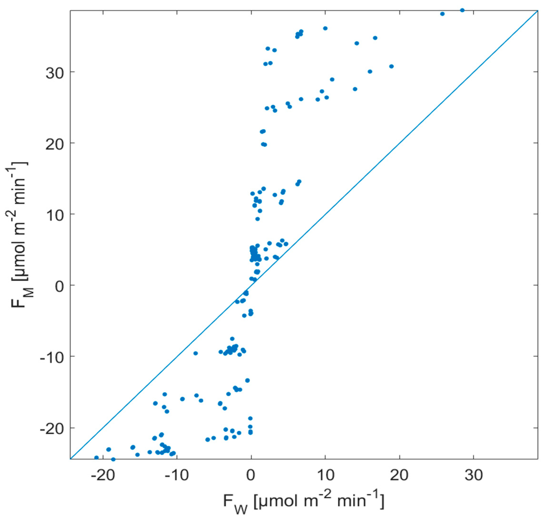
3.1.2. Comparison of Zero Intercept and Nonzero Intercept Parameterizations

We calculated FCO2 using the parameterization proposed by Wanninkhof [3] (FW) and the one from this study (FM) detailed in Table 2 and obtained from the measurement campaigns (Table 1). Figure 3 shows the relationship between the FCO2 calculated from Wanninkhof (FW) and this study (FM). FW values ranged from −21 to 28 µmol m−2 min−1, whereas FM values ranged from −29 to 43 µmol m−2 min−1. For our observations (i.e., U10 < 7 m s−1), positive FCO2 were always higher with the new parameterization, taking the nonzero intercept into account (i.e., FCO2 were above the 1:1 line), which means that source regions became stronger sources. On the other hand, negative FCO2 were always lower with the new parameterization (i.e., FCO2 are below the 1:1 line), which meant that sinks become stronger sinks. The conventional parameterization calculated an FCO2 equal to 0 (ranging from −1.7 to 2.2 µmol m−2 min−1) for low wind conditions (U10 < 2 m s−1) (Figure 4b), and the modified parameterization with the nonzero intercept had a range from −12 to 20 µmol m−2 min−1 for low wind conditions (Figure 4e).
We then present the difference between FW and FM and calculate their ratio, as it indicates how different FM is from FW. When FM/FW is equal to one, the two FCO2 are identical. If the FM/FW ratio is greater than 1, the gas transfer parameterization with a nonzero intercept leads to higher FCO2 than the parameterization without an intercept.
The ratio between FM and FW ranged from 1.4 to 124 (Figure 5). Ratios lower than 2 corresponded to wind speeds higher than 4.6 m s−1. All FCO2 computed with the nonzero intercept parameterization (FM) were higher than those computed with the conventional parameterization (FW). The highest ratios (from 6.6 to 124) corresponded to wind speeds lower than or equal to 2 m s−1. FM/FW ratios higher than 25 corresponded to wind speeds lower than 1.0 m s−1, where FW ranges from −0.1 to 0.2 µmol m−2 min−1 (Figure 4b) even if ΔpCO2 ranges from –300 to 211 µatm (Figure 4a and Figure 5a). FM exhibited a linear relationship with ΔpCO2 (Figure 4d) and a scatter for all wind speed ranges (Figure 4e).
We compared the in situ fluxes measured directly with Sniffle with the fluxes we calculated with different parametrizations. These comparisons are shown in Figure 4c, f and Table 3. Overall, the slope was close to 1 for FM (Table 3), where 1 represents perfect agreement. For FW, the slope was 0.459 (Figure 4c and Table 3). R2 and r were also higher for FM than for FW. FM used a k calculated from in situ fluxes so the two values were not completely independent. However, the differences were higher than the 10.8% uncertainty estimated for our measurements that this bias could cause.
The analysis of the Sniffle data demonstrated that the use of a nonzero intercept parameterization might improve the calculated flux. In the following sections, we tested the implications in two different frameworks: the surface ocean observation-based method and the Bern3D model. Note that the three independent approaches used in this study use very different time spans (from minutes to thousands of years). We compared the different gas transfer velocity parameterizations within one approach, not between approaches, which meant that the time span differences were not problematic.

3.2. Application of Nonzero Intercept Parameterizations within Different Frameworks

3.2.1. Use and Description of Parameterizations

We evaluated surface ocean observations with five different parameterizations and Bern3D observations with two parameterizations (see Table 2 for details). We tested the original parameterization described by Wanninkhof [3] (W) and the parameterization from this study (M) with slightly lower slopes than W based on in situ Sniffle data. We then tested (i) the original parameterization described by Wanninkhof [3] (W), (ii) the parameterization from this study (M), (iii) the parameterization described by Wanninkhof [3] with the addition of a 10.7 cm h−1 intercept (W+I) as reported in Ribas-Ribas, et al. [15] (iv) the original parameterization described by Krakauer, et al. [32] (K), and (v) the parameterization described by Krakauer, et al. [32] with the addition of an 11 cm h−1 intercept (K+I) for the surface ocean observation-based method. Finally, we modified the Bern3D Ocean Model [34] with K and K+I. Zhang and Cai [16] used a nonzero intercept of 10 cm h−1 from various studies. This is in agreement with the nonzero intercept of 10.7 cm h−1 reported by Ribas-Ribas, et al. [15]. This is the reason why we added this to W and K. For the Sniffle data analysis in Section 3.1, for clarity and brevity, we only compared the nonzero intercept parameterization from this study with the conventional parameterization from Wanninkhof. We used the five parameterizations associated with surface ocean observations presented in Table 2.
Figure 6 shows the distribution of gas transfer velocities versus wind speed, together with the wind speed histogram. We categorized the wind speed distribution into two regimes, in which different parameterizations (Table 2) produced similar k values, as follows:
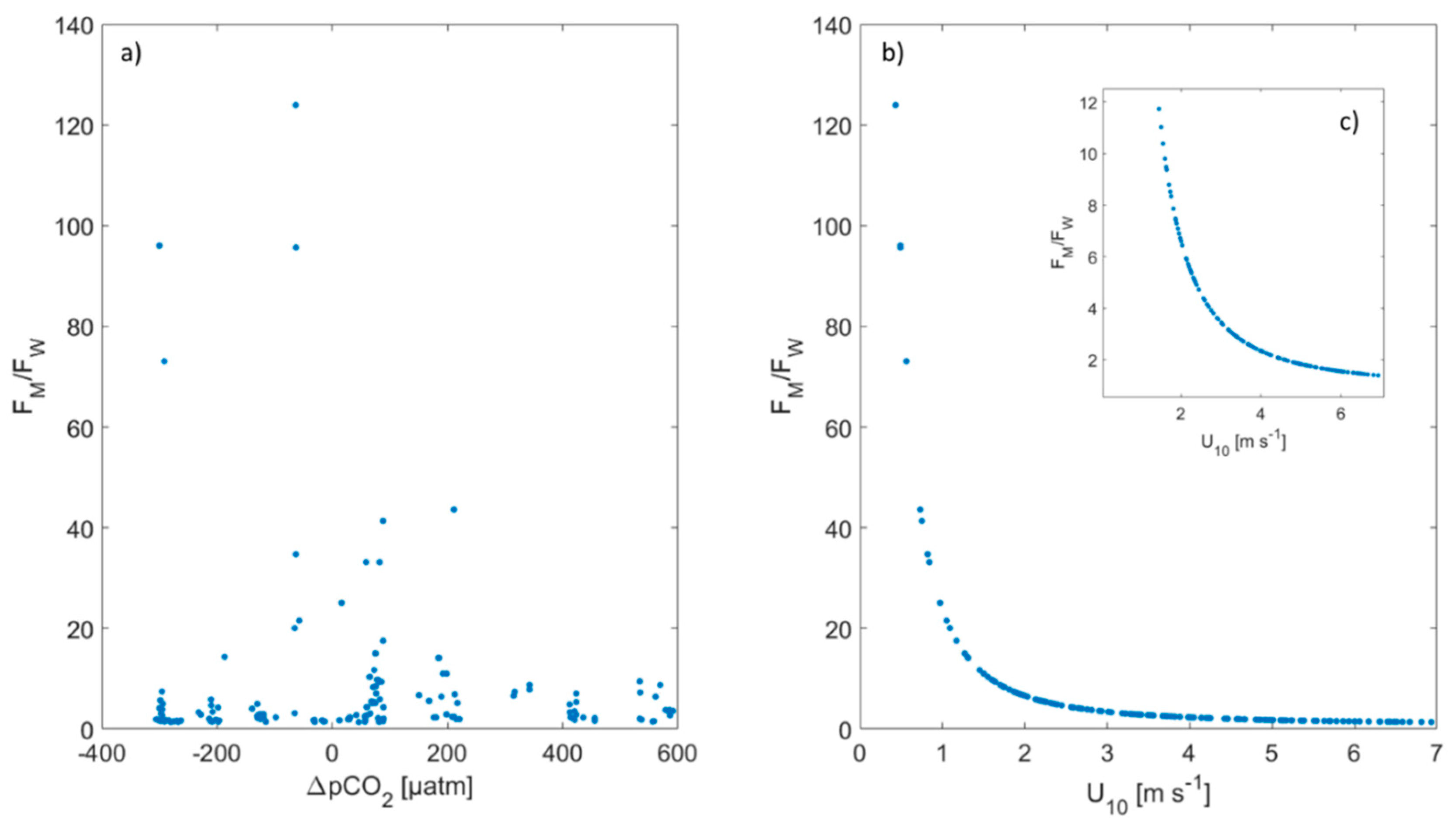
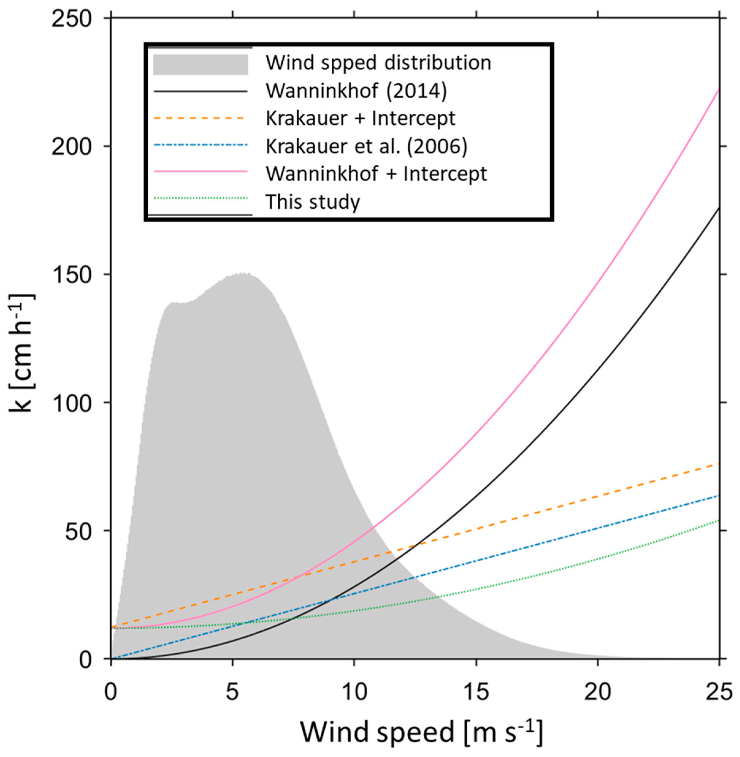
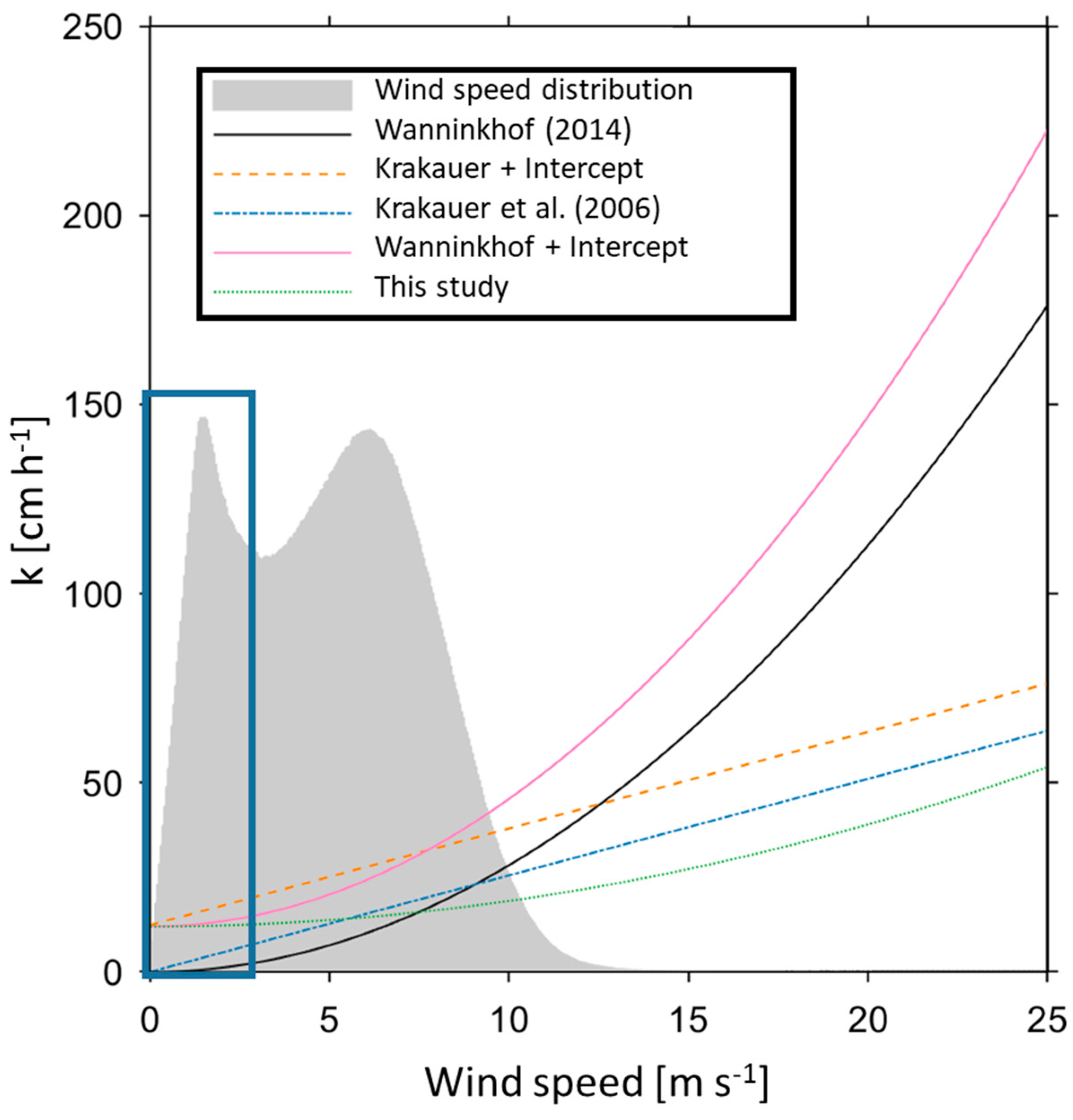
  • From 0–11 m s−1, parametrizations with a nonzero intercept were similar, and parametrizations without an intercept were similar. This was the wind region for which the implementation of a nonzero intercept was relevant for global FCO2.
  • Above 11 m s−1, the groups were quadratic parameterizations with higher slope versus linear or quadratic with lower slope. The nonzero intercept had no impact on FCO2, because bubble-mediated transport may dominate the FCO2. Therefore, this wind regime is not further discussed, and details on gas transfer at the high wind speed regimes can be found in Krall and Jähne [47], McNeil and D’Asaro [48].

3.2.2. Surface Ocean Observation-Based Method

Table 4 shows the annual mean ocean–atmosphere CO2 fluxes on the global scale and for the different regions. Integrated globally, parameterizations with a nonzero intercept yielded larger carbon fluxes between the ocean and atmosphere compared with their zero intercept parameterizations. With a nonzero intercept, the W yielded an FCO2 of −4.28 Gt C yr−1; without the intercept, the exchange flux was −2.56 Gt C yr−1 (Table 4). In general, the W+I parameterization gave higher absolute flux values except in the Tropical areas. W+I had larger k values than the other parameterizations throughout the entire wind speed range (Figure 5) except from 0 to 6 m s−1, where K+I is higher. The K gave results similar to M except for the global ocean, where M was 0.4 Gt C yr−1 lower than K (Table 4 and Figure S1). The Atlantic and Pacific (Table 4) act as a sink of CO2, and the addition of the intercept increased the sink by a factor of 1.8. The Tropical Ocean was different: ΔpCO2 was positive, so it acted as a source of CO2 to the atmosphere for the entire evaluation period (Table 4). The nonzero intercept in M indicated that fluxes were 2.2 times larger than W for regions in the Tropical Ocean (Table 4). We further evaluated the Tropical Ocean as a “case study” in the next section.

3.2.3. Tropical Ocean

Figure 7 shows the different parameterizations used in this study (as in Figure 6) with the wind histogram for the Tropical Ocean. The wind distribution differed from that of the global ocean as it had a binomial pick located at wind speeds of 2–3 m s−1 and a second pick similar to the one observed in the global distribution (Figure 6) around 6–7 m s−1. If we multiply the k parameterizations with the wind speed histogram, we obtain the relative importance of the parameterizations normalized to the actual wind speed distribution. The higher frequency of low wind speeds gave the parameterization with a nonzero intercept a higher importance than for the lower 4 m s−1 wind speed regime (see the pick in the blue square). M was close to the W+I and K+I (based on the sensitivity experiments). CO2 fluxes calculated from M are almost double FW, mostly due to the pick of wind frequency at lower wind speed. The parameterization M performed well, as it gave reasonable numbers in the global estimation and other parts of the ocean. W parameterization gave the lowest FCO2—lower than K and M because of the lower importance of high wind speed. The FCO2 calculated from K+I were the highest in the Tropics (Table 4), as it had larger k values from 0 to 6 m s−1 and low wind speeds occurred most frequently in the Tropics.

3.2.4. Bern3D Ocean Model

We ran a sensitivity simulation in a well-tested ocean model of intermediate complexity to test the implications of different gas transfer velocity parameterizations for the natural carbon cycle in the absence of anthropogenic CO2 emissions. We did not test the uncertainty of the oceanic sink for anthropogenic carbon. The importance of the gas transfer velocity for estimates of the uptake of anthropogenic carbon in ocean models has been assessed in previous studies [49,50,51], which have found that the sensitivity of the uptake to the gas exchange rate is small.

3.2.5. Global Evolution

The globally averaged FCO2 fluctuated around zero for preindustrial conditions, implying an equilibrated carbon cycle (Figure 8a). In the first few years after adding a nonzero intercept to the k, the FCO2 changed from a globally positive anomaly to a globally negative anomaly and back to globally positive anomaly (Figure 8a). After ~16 years, a globally positive FCO2 anomaly established itself, and it takes ~1000 years for this FCO2 anomaly to re-approach values of zero. Given sufficient equilibration time, the ocean approached a new equilibrium at which a zero net exchange of CO2 between ocean and atmosphere reestablishes itself. The carbon inventories in the atmosphere and ocean changed according to the perturbed global FCO2 and feedback phenomena triggered by sediment interactions. After a small decrease in atmospheric pCO2 in the first few years, atmospheric CO2 steadily increased by up to 8 ppmv, ~17 Gt C, after 5,000 years (Figure 8b).
A generally positive FCO2 anomaly over most of the simulation period caused a net transfer of carbon from the ocean to the atmosphere. The global oceanic dissolved inorganic carbon (DIC) inventory slightly increased in the first few years and decreased by ~60 Gt C as the model approached a new equilibrium state (Figure 8c). The oceanic loss of carbon was amplified by sediment interactions, and the ocean lost additional carbon to the sediments (~40 Gt C) driven by the enhanced burial of calcium carbonate. This occurred because with smaller dissolved DIC concentrations, a larger area of sediments was exposed to higher oversaturation with respect to calcium carbonate, such that more calcium carbonate was preserved within sediments. With new carbon inventories in the ocean and atmosphere, a zero net exchange between the ocean and atmosphere reestablished itself. The increase in atmospheric CO2 caused a slight warming (ΔTatm = 0.125 K) with negligible impacts on the oceanic carbon cycle and circulation (not shown). The model did not fully equilibrate after 5000 years, as exchange fluxes with sediments had an equilibration timescale on the order of 50,000 years (see, for example, Roth, et al. [41]).

3.2.6. Regional Patterns

We showed regional patterns of the FCO2 (Figure 9a) depicting the regional preindustrial steady state exchange of FCO2 between the ocean and atmosphere. The model simulated CO2 sunk in the gyre regions of all basins and in the North Atlantic and North Pacific. The Tropical Ocean and the Southern Ocean were source regions for atmospheric CO2. As stated above, globally averaged, the FCO2 was zero for preindustrial conditions.
The regional model response to increased gas transfer velocities was to amplify the general direction of preindustrial CO2 exchange between ocean and atmosphere, that is, source regions became stronger source regions (more positive anomalies), and sink regions became stronger sink regions (more negative anomalies) (Figure 9b). These anomalies were strongest in the first few years after the perturbation (Figure 9b). At the end of the simulation, when the FCO2 approached equilibrium values, there were still pronounced regional anomalies, with source regions generally becoming stronger sources and sink regions becoming stronger sinks (Figure 9c).
These anomalies caused changes in the carbon inventories of the ocean and atmosphere. The ocean globally loses 60 Gt C, with regional increases and decreases depending on the prevailing FCO2 at the surface, subsequent water transport pathways, and amplifications through sediment interactions.
In the mid-latitude and North Atlantic (i.e., generally a CO2 sink region), negative FCO2 anomalies were simulated for the natural carbon cycle. This means that the region acted as a stronger CO2 sink, which led to increased DIC concentrations in the ocean (Figure 9d). As the North Atlantic is a region of deep water formation, increased DIC anomalies spread in the Atlantic basin along the flows of deep water formation.
In the Southern Ocean, a CO2 source region, positive FCO2 anomalies were simulated. This meant that the region acted as a stronger CO2 source, which led to decreased DIC concentrations (Figure 9d). As the Southern Ocean ventilates the deep South Atlantic and most of the deep Pacific, negative DIC anomalies spread along the flows of Southern Ocean deep water (Figure 9d). This caused higher calcium carbonate preservation and additional carbon loss to sediments.
The tropical oceans, which were simulated to become stronger source regions, led to lower DIC concentrations of the surface ocean. These anomalies did not spread in the deep ocean, as these regions are characterized by upwelling.
Regions of intermediate water formation, around 30° S, which became stronger CO2 sinks, caused positive DIC anomalies in the upper ocean of the Atlantic and Pacific Oceans.
Despite small changes in the globally averaged exchange FCO2, regionally large anomalies were simulated. As the model approached a new zero net exchange equilibrium state, more pronounced regional differences in positive and negative FCO2 were simulated.

4. Discussion

We evaluated the impact on the CO2 flux using gas transfer velocity parameterization with wind speed with and without an intercept, as wind speed is the easiest and most available parameter. By doing so, we are not proposing the use of a new wind-based parameterization, as we and others have already shown that wind speed is not the best stand-alone parameter for determining gas transfer velocities [9,20,21,22], and other parameters, such as turbulent kinetic energy and surfactants, will affect the transfer. However, we maintain that this analysis is important, as assuming fluxes are close to zero when wind speed is low introduces substantial uncertainty in regional CO2 fluxes. Some of the disagreement found could be due to different spatial and temporal resolutions of observational data used for the empirical fits which make some of the most common used parametrizations appropriate for regional-to-global estimates of CO2 fluxes, but these have also been used on smaller scales. Therefore, extrapolation from a local study to regional or global scales could be erroneous due to different wind speed variability and local water chemistry.

4.1. Global Ocean-Atmospher Carbon Fluxes Based on Observations of pCO2

We compared our data-based estimates for the global ocean atmosphere exchange fluxes with those obtained by the Global Carbon Project (GCP). The GCP data-based products are based on the work of Rödenbeck, et al. [31] and Landschützer, et al. [52]. For the period 1982–2017, the mean oceanic sink was −1.85 Gt C yr−1 according to Rödenbeck, et al. [31] and −1.42 Gt C yr−1 according to Landschützer, et al. [52]. Both of the data-based products used here [33] were scaled to match the global average piston velocity. These data-based products reported in GCP yielded a CO2 uptake close to the flux calculated with the parameterization proposed by this study (FM) (i.e., −1.83 Gt C yr−1). Another source of data-based products with which we can make direct comparisons is Takahashi, et al. [53]. Takahashi, et al. [53] reported a total global FCO2 of −1.4 ± 0.7 Gt C yr−1, which is lower than the data-based products reported in GCP by Rödenbeck, et al. [31] and FM, probably because the Takahashi, et al. [53] database excluded observations made during the El Niño periods in the equatorial Pacific and those made in coastal zones. Takahashi, et al. [53] used a quadratic parameterization with a scaling factor of 0.26, which is close to W’s scaling factor of 0.251.
Globally, the FW reveals a mean FCO2 of −2.56 Gt-C yr−1 for the period 1982–2018. The FCO2 in this study using M, with a nonzero intercept, was −1.83 Gt-C yr−1. Our results from Sniffle and the SOCAT-based globally gridded dataset show that including a nonzero intercept in wind-based parameterization will make a difference in the computed ocean-atmosphere CO2 fluxes, as factors other than wind will not allow gas transfer velocities to approach zero at very calm sea conditions, such as convective mixing. However, the intercept cannot simply be added to existing parameterizations. By doing so, W+I and K+I reveal a global sink of ~−4 Gt C yr−1, which is double the mean GCP estimate. For example, the M includes the intercept, but the slope is lower, and the lower slope leads to a good match with the mean GCP data-based estimate. On a global scale, the higher slope in the W compensates for the missing intercept. However, that does not hold for the tropical oceanic regions, which exhibit a frequent occurrence of low wind regimes; that is, the application of W to tropical regions introduces an error (which is discussed further below).
On the global scale, FM reduced the oceanic uptake by 28% compared to the FW. Even with the nonzero intercepts, M gave a noticeably lower FCO2 than the K+I and W+I, due to the lower gas transfer velocities in the 5–10 m s−1 range. However, the M computed higher k values at wind speeds <5 m s−1, resulting in a better agreement of the FCO2 with the W and K than with the W+I and K+I (Figure 7 and Table 4). Generally, K+I revealed higher FCO2 than FW. Even so, W computed the highest k values above ~12 m s−1; this parameterization estimated lower k values in the low wind regimes (<4 m s−1) than do the K and M.
We suggest that the behavior of parameterizations in the low wind speed regime is crucial in the computation of regional FCO2 due to the relatively high frequency of the occurrence of wind speeds below 4 m s−1 compared with wind speeds above 10 m s−1 [5]. For the global analysis of the data product, the nonzero intercept parameterization led to a lower CO2 uptake (Table 4).
It is interesting to note that W and K reveal similar results, despite the extensive debate in the literature about whether parameterizations should be based on linear, quadratic, or cubic relationships with wind [22]. In future work, it is recommended to run similar analysis with other parametrizations, such as with parameterizations developed for coastal waters.

4.2. Regional Patterns

FCO2 estimations from the surface ocean observation-based method range in general from −0.02 to −0.04 Gt C yr−1 (Table 4). This range is in close agreement with the mean annual flux of −0.06 Pg C yr−1 in the ice-free zone of the Southern Ocean [53] but an order of magnitude lower than the FCO2 estimate from McNeil, et al. [54]. Different parameterizations give different ranges, which means that the FCO2 estimation will be stronger in sources or sinks depending on the season. Takahashi, et al. [53] also claimed that their flux was small due to the cancellation of the summer uptake of FCO2 with the winter release of CO2 caused by deep-water upwelling.
In the Tropical Ocean, wind speeds were more frequently below 5 m s−1 compared with other global oceanic regions, with the consequence being that ignoring nonzero intercepts led to differences of 32% (Figure 7). Takahashi, et al. [53] reported that the equatorial Pacific is the major oceanic source of atmospheric CO2 (+0.48 Pg C yr−1), which agrees well with FM for tropical oceanic regions (+0.43 Pg C yr−1) (Table 4). From Sniffle and the regional results of the surface ocean observation-based method, we can conclude that the parameterizations without an intercept underestimate the FCO2 in low wind speed regimes. For example, the difference between FW and FM in the tropics is 0.16 Gt C yr−1, in agreement with the value of 0.2 Pg C yr−1 reported by Zhang and Cai [16] with an estimated nonzero intercept of 10 cm h−1. That means a 57% increase of FCO2 in the tropical region (Table 4).

4.3. Inference of Nonzero Intercept Parameterizations Based on Observations

The nonzero intercept, reported here between 5 and 11 cm h−1, may vary among different regions with changing biogeochemical forcing. For example, Frankignoulle, et al. [13] reported a nonzero intercept of 15 cm h−1 in coral reef systems. On the other hand, some observations have indicated a smaller nonzero intercept (~1–3 cm h−1) for nonequatorial regions [11,14,55]. Encountering low wind regimes during research cruises is challenging to plan for, and some techniques lack the sensitivity to record the slow and small change in gas transfer velocities under low wind conditions. In addition, the operations of research vessels are expensive, with the general aim of covering a large observational region within the shortest time frame possible. Therefore, future oceanic studies should be conducted in regions that offer a high probability of encountering low wind speeds and large ΔpCO2 conditions. Furthermore, multidisciplinary research is required to advance the understanding of the mechanisms of processes driving gas exchange in low wind regimes. Crusius and Wanninkhof [56] found that transfer velocity and low wind speeds do not have a unique relationship, and they suggested that other processes, such as convective cooling [57], chemical enhancement [58], variations in fetch, the presence or absence of organic surface films [59], or rain [60], also affect the k. In particular, the buoyancy fluxes in low wind regimes can be important, as pointed out by MacIntyre, et al. [61]. For example, McGillis, et al. [10] suggested that their 8 cm h1 nonzero intercept was due to the buoyancy fluxes associated with a strong diurnal warming cycle. Buoyancy fluxes will affect surface turbulence, and they can be parameterized based on heat and momentum fluxes [62].
Zhang and Cai [16] estimated the ocean-atmosphere CO2 flux by adding a constant of 10 cm h−1 from previously published papers [10,17,18,19]. In agreement with our study, they reported that under low wind speed conditions, frequently found at low latitudes, wind speed may not even be the most dominant parameter for k. Zhang and Cai [16] also pointed out that not only the high ΔpCO2 (due to upwelling) in the low latitudes but also the large oceanic coverage at low latitudes will significantly underestimate the CO2 flux in the equatorial areas.
The observations with FM/FW ratios higher than 25 correspond to coastal stations (offshore Australia, Jade Bay, the Baltic Sea, and Norwegian fjords) (Figure 5). It is not reasonable to assume that the flux is close to zero when large ΔpCO2 and low wind speeds are observed (Figure 4 and Figure 5) due to the presence other factors driving gas exchange, as discussed above. The mismatch between oceanic and coastal observation, based on our FM/FW ratios, could be one of the reasons why there has been extensive debate in the literature about whether coastal regions act as a source or sink of CO2 [63]. Coastal systems are highly dynamic, and different conditions, such as upwelling, tidal influence, fresh water discharge, and fetch, are likely to be driving forces of gas transfer velocities. In addition, authors have claimed that specific parameterizations for gas transfer velocities should be used for coastal/estuarine regions [64]. For example, Borges, et al. [65] found that water currents contribute significantly to the k in the Scheldt estuary and that the k has a good linear relationship with wind speed and an intercept of 4 cm h−1. Borges, et al. [12] also found a significant linear relationship between k and wind speed for the Randers Fjord and the Scheldt and Thames estuaries. The y-intercept varied from 1.2 to 9.7 cm h−1, and these differences are related to varying contributions of tidal currents to water turbulence at the interface and fetch limitation.
The way the nonzero intercept is calculated or reported has varied between authors. Some authors have used the individual wind speed data [9] and others have binned the wind speed into different regimes [62,66,67]. Another difference is how the y-intercept is calculated. Most commonly, it is done by fitting the gas transfer velocities to the whole range of wind speed [3,9,12,60]. However, this fitting approach could be influenced by data in the higher wind regimes and, therefore, lead to an overestimation of the intercept. In order to reduce this artifact, Butterworth and Miller [11] determined the y-intercept by linear extrapolation of the two lowest wind speed bins.

4.4. Implications in Ocean Models

Although an accurate representation of the gas transfer velocity is crucial to estimating the current uptake of carbon from pCO2-based observations [7,8,53], it has been shown to be of secondary importance for estimating the anthropogenic uptake of CO2 in ocean models; the oceanic uptake of anthropogenic CO2 in ocean models is driven primarily by increasing atmospheric CO2 and is limited mainly by its transport from the surface to deep water [49,50,51]. 14CO2 and 13CO2, on the other hand, which have longer equilibration timescales with the surface ocean compared to CO2 [68], are affected by different gas transfer velocities in models, and uncertainties in the gas transfer velocity are therefore critical for the analysis of carbon isotopes. Three-dimensional global ocean models have therefore been applied in combination with a range of suitable data-based metrics to infer the gas exchange velocity parameterization. Krakauer, et al. [32], for instance, used oceanic and atmospheric observations of 14C and 13C to constrain the gas exchange parameterization, utilizing the distinct signatures left by the ocean-atmosphere exchange of 14CO2 and 13CO2 in their model. Bern3D has adopted the relationship proposed by Krakauer, et al. [32] and further updated the relationship proposed by Müller, et al. [46] to best reproduce a suite of data-based metrics.
The simulations presented in this study assess how the natural carbon cycle in an ocean model adjusts to a perturbation of the gas transfer velocity. In response to a faster transfer velocity, source regions tend to become stronger sources and sink regions tend to become stronger sink regions. Transiently, this leads to a net transfer of carbon from the ocean to the atmosphere, but the system eventually reaches a new equilibrium at which the global sources and sinks balance each other again. Towards the end of the simulations, an equilibrated system at the global scale is reached. Regionally, however, stronger gradients are simulated between the source and sink regions.

5. Conclusions

It is clear that a nonzero intercept is crucial to computing CO2 fluxes in low wind regimes based on observations of pCO2, especially in the Tropics. Nevertheless, more systematic and multidisciplinary studies of in situ gas transfer velocities, together with investigations of buoyancy fluxes, surface films, and rain in different regions and conditions, are required to understand the mechanisms and variability of gas transfer across the ocean’s surface. Autonomous platforms and satellite missions have the potential to fill temporal and spatial gaps in future observations. Uncertainties in the gas transfer velocity are of secondary importance for estimating the anthropogenic uptake of carbon in ocean models.

Supplementary Materials

The following are available online at https://www.mdpi.com/2076-3263/9/5/230/s1: Figure S1: Fluxes calculated from the pCO2-based product for the period 1982–2018. (a) Global and from (b) to (f) where higher changes are expected: (b) Southern Ocean, (c) North Atlantic, (d) Tropical, (e) South Atlantic, and (f) South Pacific. Different colors represent different parameterizations, as in Figure 5: black indicates FW, blue indicates FK, orange indicates FK+I, rose indicates FW+I, and green indicates FM. The color legend is the same as in Figure 6 of the main test.

Author Contributions

Conceptualization, M.R.-R.; methodology, M.R.-R., G.B., and M.P.H.; writing—original draft preparation, M.R.-R.; writing—review & editing, M.R.-R., G.B., M.P.H., and O.W.; funding acquisition, O.W.

Funding

This research was funded by the European Research Council (ERC) grant number [GA336408].

Acknowledgments

We thank the Schmidt Ocean Institute (SOI), the captains and the crews of R/Vs Senckenberg, Otzum, Zephyr, Meteor, Falkor, Heincke, and Elisabeth Mann Borgese. Many thanks to all scientific crew members on board for their support during both cruises, especially to Hanne Marie Banko-Kubis and Nur Ili Hamizah Mustaffa. The Surface Ocean CO2 Atlas (SOCAT) is an international effort, endorsed by the International Ocean Carbon Coordination Project (IOCCP), the Surface Ocean Lower Atmosphere Study (SOLAS), and the Integrated Marine Biosphere Research (IMBeR) program, to deliver a uniformly quality-controlled surface ocean CO2 database. The many researchers and funding agencies responsible for the collection of data and quality control are thanked for their contributions to SOCAT.

Conflicts of Interest

The authors declare no conflict of interest. The funders had no role in the design of the study, in the collection, analyses, or interpretation of data, in the writing of the manuscript, or in the decision to publish the results.

References

  1. Le Quéré, C.; Andrew, R.M.; Friedlingstein, P.; Sitch, S.; Hauck, J.; Pongratz, J.; Pickers, P.A.; Korsbakken, J.I.; Peters, G.P.; Canadell, J.G.; et al. Global carbon budget 2018. Earth Syst. Sci. Data 2018, 10, 2141–2194. [Google Scholar]
  2. Weiss, R.F. Carbon dioxide in water and seawater: The solubility of a non–ideal gas. Mar. Chem. 1974, 2, 203–215. [Google Scholar] [CrossRef]
  3. Wanninkhof, R. Relationship between wind speed and gas exchange over the ocean revisited. Limnol. Oceanogr. Methods 2014, 12, 351–362. [Google Scholar] [CrossRef] [Green Version]
  4. Johnson, M.T. A numerical scheme to calculate temperature and salinity dependent air–water transfer velocities for any gas. Ocean Sci. 2010, 6, 913–932. [Google Scholar] [CrossRef]
  5. Archer, C.L.; Jacobson, M.Z. Evaluation of global wind power. J. Geophys. Res. Atmos. 2005, 110, D12110. [Google Scholar] [CrossRef]
  6. Wurl, O.; Stolle, C.; Van Thuoc, C.; The Thu, P.; Mari, X. Biofilm-like properties of the sea surface and predicted effects on air-sea CO2 exchange. Prog. Oceanogr. 2016, 144, 15–24. [Google Scholar] [CrossRef]
  7. Rödenbeck, C.; Bakker, D.C.E.; Gruber, N.; Iida, Y.; Jacobson, A.R.; Jones, S.; Landschützer, P.; Metzl, N.; Nakaoka, S.; Olsen, A.; et al. Data-based estimates of the ocean carbon sink variability – first results of the surface ocean pCO2 mapping intercomparison (socom). Biogeosciences 2015, 12, 7251–7278. [Google Scholar]
  8. Landschützer, P.; Gruber, N.; Bakker, D.; Schuster, U. Recent variability of the global ocean carbon sink. Global Biogeochem. Cy. 2014, 28, 927–949. [Google Scholar] [CrossRef] [Green Version]
  9. Mustaffa, N.I.H.; Ribas-Ribas, M.; Banko-Kubis, H.M.; Wurl, O. In situ CO2 transfer velocity reduction by natural surfactants in the sea surface microlayer. in preparation.
  10. McGillis, W.R.; Edson, J.B.; Zappa, C.J.; Ware, J.D.; McKenna, S.P.; Terray, E.A.; Hare, J.E.; Fairall, C.W.; Drennan, W.; Donelan, M. Air-sea CO2 exchange in the equatorial pacific. J. Geophys. Res. Oceans 2004, 109, C08S02. [Google Scholar] [CrossRef]
  11. Butterworth, B.J.; Miller, S.D. Air-sea exchange of carbon dioxide in the southern ocean and antarctic marginal ice zone. Geophys. Res. Lett. 2016, 43, 7223–7230. [Google Scholar] [CrossRef]
  12. Borges, A.V.; Delille, B.; Schiettecatte, L.-S.; Gazeau, F.; Abril, G.; Frankignoulle, M. Gas transfer velocities of CO2 in three european estuaries (randers fjord, scheldt, and thames). Limnol. Oceanogr. 2004, 49, 1630–1641. [Google Scholar] [CrossRef]
  13. Frankignoulle, M.; Gattuso, J.-P.; Biondo, R.; Bourge, I.; Copin-Montégut, G.; Pichon, M. Carbon fluxes in coral reefs. Ii. Eulerian study of inorganic carbon dynamics and measurement of air-sea CO2 exchanges. Mar. Ecol. Prog. Ser. 1996, 145, 123–132. [Google Scholar] [CrossRef]
  14. Kremer, J.N.; Reischauer, A.; D’Avanzo, C. Estuary-specific variation in the air-water gas exchange coefficient for oxygen. Estuaries Coasts 2003, 26, 829–836. [Google Scholar] [CrossRef]
  15. Ribas-Ribas, M.; Helleis, F.; Rahlff, J.; Wurl, O. Air-sea CO2-exchange in a large annular wind-wave tank and the effects of surfactants. Front. Mar. Sci. 2018, 5, 457. [Google Scholar] [CrossRef]
  16. Zhang, X.; Cai, W.J. On some biases of estimating the global distribution of air-sea CO2 flux by bulk parameterizations. Geophys. Res. Lett. 2007, 34. [Google Scholar] [CrossRef]
  17. Soloviev, A.; Schluessel, P. A model of air-sea gas exchange incorporating the physics of the turbulent boundary layer and the properties of the sea surface. In Gas Transfer at Water Surfaces; Donelan, M., Ed.; AGU: Washington, DC, USA, 2002; Volume 127, pp. 141–146. [Google Scholar]
  18. Monahan, E.C.; Spillane, M.C. The role of oceanic whitecaps in air-sea gas exchange. In Gas Transfer at Water Surfaces; Brutsaert, W., Jirka, G.H., Eds.; Springer: New York, NY, USA, 1984; pp. 495–503. [Google Scholar]
  19. Asher, W.E.; Jessup, A.T.; Atmane, M.A. Oceanic application of the active controlled flux technique for measuring air-sea transfer velocities of heat and gases. J. Geophys. Res. Oceans 2004, 109. [Google Scholar] [CrossRef] [Green Version]
  20. Banko-Kubis, H.M.; Wurl, O.; Mustaffa, N.I.H.; Ribas-Ribas, M. Gas transfer velocities in norwegian fjords and the adjacent north atlantic waters. Oceanologia 2019, 61. [Google Scholar] [CrossRef]
  21. Zappa, C.J.; McGillis, W.R.; Raymond, P.A.; Edson, J.B.; Hintsa, E.J.; Zemmelink, H.J.; Dacey, J.W.; Ho, D.T. Environmental turbulent mixing controls on air–water gas exchange in marine and aquatic systems. Geophys. Res. Lett. 2007, 34, L10601. [Google Scholar] [CrossRef]
  22. Wanninkhof, R.; Asher, W.E.; Ho, D.T.; Sweeney, C.; McGillis, W.R. Advances in quantifying air–sea gas exchange and environmental forcing. Annu. Rev. Marine Sci. 2009, 1, 213–244. [Google Scholar] [CrossRef]
  23. Ribas-Ribas, M.; Kilcher, L.F.; Wurl, O. Sniffle: A step forward to measure in situ CO2 fluxes with the floating chamber technique. Elem. Sci. Anth. 2018, 6, 14. [Google Scholar] [CrossRef]
  24. Ribas-Ribas, M.; Mustaffa, N.I.H.; Rahlff, J.; Stolle, C.; Wurl, O. Sea surface scanner (s3): A catamaran for high–resolution measurements of biogeochemical properties of the sea surface microlayer. J. Atmos. Ocean Tech. 2017, 34, 1433–1448. [Google Scholar] [CrossRef]
  25. Stolle, C.; Ribas-Ribas, M.; Badewien, T.H.; Carpenter, L.J.; Chance, R.; Damgaard, L.R.; Quesada, A.M.D.; Engel, A.; Frka, S.; Galgani, L.; et al. The milan campaign: Studying diel light effects on the air-sea interface. B Am. Meteorol. Soc. under revision.
  26. Mesarchaki, E.; Kräuter, C.; Krall, K.; Bopp, M.; Helleis, F.; Williams, J.; Jähne, B. Measuring air–sea gas-exchange velocities in a large-scale annular wind–wave tank. Ocean Sci. 2015, 11, 121–138. [Google Scholar] [CrossRef] [Green Version]
  27. Taylor, J. Introduction to Error Analysis, the Study of Uncertainties in Physical Measurements; University Science Book: Sausalito, CA, USA, 1997. [Google Scholar]
  28. Rödenbeck, C.; Keeling, R.F.; Bakker, D.C.E.; Metzl, N.; Olsen, A.; Sabine, C.; Heimann, M. Global surface-ocean pCO2 and sea–air CO2 flux variability from an observation-driven ocean mixed-layer scheme. Ocean Sci. 2013, 9, 193–216. [Google Scholar] [CrossRef]
  29. Bakker, D.C.E.; Pfeil, B.; Landa, C.S.; Metzl, N.; O’Brien, K.M.; Olsen, A.; Smith, K.; Cosca, C.; Harasawa, S.; Jones, S.D.; et al. A multi-decade record of high-quality fCO2 data in version 3 of the surface ocean CO2 atlas (socat). Earth Syst. Sci. Data 2016, 8, 383–413. [Google Scholar] [CrossRef]
  30. Dee, D.; Uppala, S.; Simmons, A.; Berrisford, P.; Poli, P.; Kobayashi, S.; Andrae, U.; Balmaseda, M.; Balsamo, G.; Bauer, P. The era-interim reanalysis: Configuration and performance of the data assimilation system. QJ Roy. Meteor. Soc. 2011, 137, 553–597. [Google Scholar] [CrossRef]
  31. Rödenbeck, C.; Bakker, D.C.E.; Metzl, N.; Olsen, A.; Sabine, C.; Cassar, N.; Reum, F.; Keeling, R.F.; Heimann, M. Interannual sea–air CO2 flux variability from an observation-driven ocean mixed-layer scheme. Biogeosciences 2014, 11, 4599–4613. [Google Scholar] [CrossRef]
  32. Krakauer, N.Y.; Randerson, J.T.; Primeau, F.W.; Gruber, N.; Menemenlis, D. Carbon isotope evidence for the latitudinal distribution and wind speed dependence of the air–sea gas transfer velocity. Tellus 2006, 58B, 390–417. [Google Scholar] [CrossRef]
  33. Wanninkhof, R. Relationship between wind speed and gas exchange over the ocean. J. Geophys. Res. 1992, 97, 7373–7382. [Google Scholar] [CrossRef]
  34. Müller, S.; Joos, F.; Edwards, N.; Stocker, T. Water mass distribution and ventilation time scales in a cost-efficient, three-dimensional ocean model. J. Clim. 2006, 19, 5479–5499. [Google Scholar] [CrossRef]
  35. Griffies, S.M. The gent–mcwilliams skew flux. J. Phys. Oceanogr. 1998, 28, 831–841. [Google Scholar] [CrossRef]
  36. Ritz, S.P.; Stocker, T.F.; Joos, F. A coupled dynamical ocean–energy balance atmosphere model for paleoclimate studies. J. Clim. 2011, 24, 349–375. [Google Scholar] [CrossRef]
  37. Tschumi, T.; Joos, F.; Gehlen, M.; Heinze, C. Deep ocean ventilation, carbon isotopes, marine sedimentation and the deglacial CO2 rise. Clim. Past 2011, 6, 1895–1958. [Google Scholar] [CrossRef]
  38. Parekh, P.; Joos, F.; Müller, S.A. A modeling assessment of the interplay between aeolian iron fluxes and iron-binding ligands in controlling carbon dioxide fluctuations during antarctic warm events. Paleoceanography 2008, 23. [Google Scholar] [CrossRef]
  39. Kalnay, E.; Kanamitsu, M.; Kistler, R.; Collins, W.; Deaven, D.; Gandin, L.; Iredell, M.; Saha, S.; White, G.; Woollen, J. The ncep/ncar 40-year reanalysis project. B Am. Meteorol. Soc. 1996, 77, 437–471. [Google Scholar] [CrossRef]
  40. Roth, R. Modeling forcings and responses in the global carbon cycle-climate system: Past, present and future. Verlag nicht ermittelbar, 2013. Available online: http://work.bergophil.ch/roth13phd.pdf (accessed on 15 May 2019).
  41. Roth, R.; Ritz, S.P.; Joos, F. Burial-nutrient feedbacks amplify the sensitivity of atmospheric carbon dioxide to changes in organic matter remineralisation. Earth Syst. Dyn. 2014, 5, 321–343. [Google Scholar] [CrossRef] [Green Version]
  42. Battaglia, G.; Steinacher, M.; Joos, F. A probabilistic assessment of calcium carbonate export and dissolution in the modern ocean. Biogeosciences 2016, 13, 2823–2848. [Google Scholar] [CrossRef] [Green Version]
  43. Najjar, R.; Orr, J. Biotic—howto, Internal Ocmip Report; LSCE/CEA Saclay: Gifsur-Yvette, France, 1999. [Google Scholar]
  44. Orr, J.; Najjar, R.; Sabine, C.; Joos, F. Abiotic-howto, Internal Ocmip Report; LSCE/CEA Saclay: Gifsur-Yvette, France, 1999. [Google Scholar]
  45. Orr, J.; Epitalon, J.-M. Improved routines to model the ocean carbonate system: Mocsy 2.0. Geosci. Model Dev. 2015, 8, 485–499. [Google Scholar] [CrossRef]
  46. Müller, S.; Joos, F.; Plattner, G.K.; Edwards, N.; Stocker, T. Modeled natural and excess radiocarbon: Sensitivities to the gas exchange formulation and ocean transport strength. Global Biogeochem. Cy. 2008, 22. [Google Scholar] [CrossRef] [Green Version]
  47. Krall, K.E.; Jähne, B. First laboratory study of air–sea gas exchange at hurricane wind speeds. Ocean Sci. 2014, 10, 257–265. [Google Scholar] [CrossRef] [Green Version]
  48. McNeil, C.; D’Asaro, E. Parameterization of air–sea gas fluxes at extreme wind speeds. J. Marine Syst. 2007, 66, 110–121. [Google Scholar] [CrossRef]
  49. Sarmiento, J.L.; Orr, J.C.; Siegenthaler, U. A perturbation simulation of CO2 uptake in an ocean general circulation model. J. Geophys. Res. Oceans 1992, 97, 3621–3645. [Google Scholar] [CrossRef]
  50. Graven, H.D.; Gruber, N.; Key, R.; Khatiwala, S.; Giraud, X. Changing controls on oceanic radiocarbon: New insights on shallow-to-deep ocean exchange and anthropogenic CO2 uptake. J. Geophys. Res. Oceans 2012, 117, C10005. [Google Scholar] [CrossRef]
  51. Ciais, P.; Sabine, C.; Bala, G.; Bopp, L.; Brovkin, V.; Canadell, J.G.; Chhabra, A.; DeFries, R.; Galloway, J.; Heimann, M.; et al. Carbon and other biogeochemical cycles. In Climate Change 2013: The Physical Science Basis. Contribution of Working Group i to the Fifth Assessment Report of the Intergovernmental Panel on Climate Change; Stocker, T., Qin, D., Plattner, G.-K., Tignor, M., Allen, S.K., Boschung, J., Nauels, A., Xia, Y., Bex, V., Midgley, P.M., Eds.; Cambridge University Press: Cambridge, UK; New York, NY, USA, 2013. [Google Scholar]
  52. Landschützer, P.; Gruber, N.; Haumann, F.A.; Rödenbeck, C.; Bakker, D.C.; Van Heuven, S.; Hoppema, M.; Metzl, N.; Sweeney, C.; Takahashi, T. The reinvigoration of the southern ocean carbon sink. Science 2015, 349, 1221–1224. [Google Scholar] [CrossRef]
  53. Takahashi, T.; Sutherland, S.C.; Wanninkhof, R.; Sweeney, C.; Feely, R.A.; Chipman, D.W.; Hales, B.; Friederich, G.; Chavez, F.; Sabine, C. Climatological mean and decadal change in surface ocean pCO2, and net sea–air CO2 flux over the global oceans. Deep Sea Res. Part. II: Top. Stud. Oceanogr. 2009, 56, 554–577. [Google Scholar] [CrossRef]
  54. McNeil, B.I.; Metzl, N.; Key, R.M.; Matear, R.J.; Corbiere, A. An empirical estimate of the southern ocean air-sea CO2 flux. Global Biogeochem. Cy. 2007, 21. [Google Scholar] [CrossRef]
  55. Donelan, M.; Wanninkhof, R. Gas transfer at water surfaces—concepts and issues. In Gas Transfer at Water Surfaces; Donelan, M., Drennan, W.M., Saltzman, E.S., Eds.; American Geophysical Union: Washington, DC, USA, 2001; pp. 1–10. [Google Scholar]
  56. Crusius, J.; Wanninkhof, R. Gas transfer velocities measured at low wind speed over a lake. Limnol. Oceanogr. 2003, 48, 1010–1017. [Google Scholar] [CrossRef] [Green Version]
  57. Crill, P.M.; Bartlett, K.B.; Wilson, J.O.; Sebacher, D.I.; Harriss, R.C.; Melack, J.M.; MacIntyre, S.; Lesack, L.; Smith-Morrill, L. Tropospheric methane from an amazonian floodplain lake. J. Geophys. Res. Atmos. 1988, 93, 1564–1570. [Google Scholar] [CrossRef]
  58. Wanninkhof, R.; Knox, M. Chemical enhancement of CO2 exchange in natural waters. Limnol. Oceanogr. 1996, 41, 689–697. [Google Scholar] [CrossRef]
  59. Frew, N.M.; Bock, E.J.; Schimpf, U.; Hara, T.; Haußecker, H.; Edson, J.B.; McGillis, W.R.; Nelson, R.K.; McKenna, S.P.; Uz, B.M. Air–sea gas transfer: Its dependence on wind stress, small–scale roughness, and surface films. J. Geophys. Res. Oceans 2004, 109, C08S17. [Google Scholar] [CrossRef]
  60. Ho, D.T.; Asher, W.E.; Bliven, L.F.; Schlosser, P.; Gordan, E.L. On mechanisms of rain-induced air-water gas exchange. J. Geophys. Res. Oceans 2000, 105, 24045–24057. [Google Scholar] [CrossRef] [Green Version]
  61. MacIntyre, S.; Eugster, W.; Kling, G.W. The critical importance of buoyancy flux for gas flux across the air-water interface. Geophysical Monograph-American Geophysical Union 2002, 127, 135–140. [Google Scholar]
  62. Fairall, C.; Hare, J.; Edson, J.; McGillis, W. Parameterization and micrometeorological measurement of air–sea gas transfer. Boundary Layer Meteorol. 2000, 96, 63–106. [Google Scholar] [CrossRef]
  63. Chen, C.-T.A.; Borges, A.V. Reconciling opposing views on carbon cycling in the coastal ocean: Continental shelves as sinks and near-shore ecosystems as sources of atmospheric CO2. Deep Sea Res. Part. II: Top. Stud. Oceanogr. 2009, 56, 578–590. [Google Scholar] [CrossRef]
  64. Raymond, P.A.; Cole, J.J. Gas exchange in rivers and estuaries: Choosing a gas transfer velocity. Estuaries 2001, 24, 312–317. [Google Scholar] [CrossRef]
  65. Borges, A.V.; Vanderborght, J.-P.; Schiettecatte, L.-S.; Gazeau, F.; Ferrón-Smith, S.; Delille, B.; Frankignoulle, M. Variability of the gas transfer velocity of CO2 in a macrotidal estuary (the scheldt). Estuaries 2004, 27, 593–603. [Google Scholar] [CrossRef]
  66. Cole, J.J.; Caraco, N.F. Atmospheric exchange of carbon dioxide in a low-wind oligotrophic lake measured by the addition of sf6. Limnol. Oceanogr. 1998, 43, 647–656. [Google Scholar] [CrossRef]
  67. McGillis, W.R.; Edson, J.B.; Hare, J.E.; Fairall, C.W. Direct covariance air-sea CO2 fluxes. J. Geophys. Res. Oceans 2001, 106, 16729–16745. [Google Scholar] [CrossRef]
  68. Broecker, W.S.; Peng, T.H. Tracers in the Sea; Lamont-Doherty Geological Observatory: Palisades, NY, USA, 1982. [Google Scholar]
Figure 1. Diagram of the Sniffle, an autonomous drifting buoy with floating chamber to measure ocean-atmosphere CO2 fluxes. Its main components are the control unit, the floating chamber, two acoustic Doppler velocimeters and the CO2 sensor. The dimensions are in cm.
Geosciences 09 00230 g001
Figure 2. Distribution of in situ k660 (plotted mean of each wind bin and error bars are the standard error of the mean) versus binned wind speed (U10). The black line shows quadratic regression in our study, k660 = 5.71 (±1.28) + 0.23 (±0.06) * U102. (R2 = 0.172, p < 0.001, n = 245). (a). Distribution of the wind speed during field measurements (b).
Geosciences 09 00230 g002
Figure 3. Comparison between a zero intercept parameterization following Wanninkhof [3] (FW) and the nonzero intercept parameterization proposed in this study (FM). The nonzero intercept parameterization resulted from a least squares regression fit to gas transfer velocity versus wind speed. Fluxes for both parameterizations were calculated with the ancillary data from the measurement campaigns presented in Table 1. The line of perfect agreement (1:1 line) is also shown.
Geosciences 09 00230 g003
Figure 4. CO2 flux calculated from the commonly used parameterization (FW) (ac) and from the parameterization with a nonzero intercept (FM) (df) versus the ocean pCO2 minus the atmospheric pCO2pCO2) (a,d), versus wind speed normalized at 10 m (b,e), and versus the flux measured in situ from Sniffle during different cruises (c,f).
Geosciences 09 00230 g004
Figure 5. Ratio between flux calculated from the normally used parameterization (FW) and from the parameterization with a nonzero intercept (FM) versus ocean pCO2 minus the atmospheric pCO2pCO2) (a) and the wind speed normalized at 10 m (b). The insert in (b) is the zoom for lower ratio to see the asymptote.
Geosciences 09 00230 g005
Figure 6. Relationship between gas transfer velocity parameterizations and wind speed and the histogram of global wind distribution for the year 2000 as an example.
Geosciences 09 00230 g006
Figure 7. Same as Figure 6 but containing the wind histogram from the Tropics from the year 2000.
Geosciences 09 00230 g007
Figure 8. Bern3D simulations of how carbon fluxes and carbon pools evolve after introducing a nonzero intercept gas transfer velocity of CO2. (a) Global ocean to atmosphere flux of CO2. (b) Atmospheric pCO2. (c) Global dissolved inorganic carbon inventory for a control run (blue) with the use of [32] and the sensitivity experiment (orange) with the addition of the nonzero intercept.
Geosciences 09 00230 g008aGeosciences 09 00230 g008b
Figure 9. Maps and section of variables of interest as simulated by the Bern3D ocean model. (a) Ocean-atmosphere flux of CO2 for preindustrial steady state conditions. (b) Changes in the ocean-atmosphere flux of CO2 in the first year after introducing a nonzero intercept for the gas transfer velocity of CO2. (c) Changes in the ocean-atmosphere flux of CO2 for new steady state conditions (year 5000). (d) Changes in dissolved inorganic carbon concentrations in a section through the Atlantic (25° W), across the Southern Ocean (58° S), and into the Pacific (175° W) for new steady state conditions. Changes are expressed relative to a control run that used a zero intercept parameterization [37].
Geosciences 09 00230 g009
Table 1. Cruise names, research vessels, dates, areas of observation, number of quality-controlled gas transfer observations, and studies that have discussed the cruises in more detail.
Cruise IDResearch VesselsStart DateEnd DateYearArea# obsRef.
M117Meteor1 August12 August2015Baltic Sea19
FK161010Falkor12 October6 November2016Timor Sea60[9]
HE491Heincke10 July25 July2017Norwegian fjords & coastal North Atlantic47[9,20]
EMB184Elisabeth Mann Borgese1 June10 June2018Baltic Sea56
31 March2 August2016Jade Bay *34[23]
3 April4 September2017Jade Bay *29[25]
* Single daily samplings from different small boats, not a cruise.
Table 2. List of gas transfer velocities parameterization (with equation, units, and references) used in Sniffle, the surface ocean observation–based method (SOCAT), and Bern3D evaluations.
Parameterization NameReference Equation   *   ( S c 660 ) 0.5 [ cm   s 1 ] Used in:
Wanninkhof (W)[3]kW = 0.251 U102Sniffle & SOCAT
This study kM = 5.7 + 0.23 U102Sniffle & SOCAT
Wanninkhof + Intercept (W+I)[15]kW+I = 10.7 + 0.30 U102SOCAT
Krakauer (K)[32]kK = 2.275 * U10SOCAT & Bern3D
Krakauer + Intercept (K+I) kK+I = 11 + 2.275 * U10SOCAT & Bern3D
Table 3. Results of the comparison between direct measurements and calculated fluxes. r is Pearson’s correlation coefficient, RMSE is root mean square error, and R-squared is the coefficient of determination. The equation that better fits the relationship with in situ fluxes with slope P1 and intercept P2 is shown with 95% confidence bounds in parentheses.
Comparison StatisticsFX = P1 * F Insitu + P2
rRMSER-SquaredP1P2
FM0.91226.91420.8320.881 (0.831, 0.931)2.928 (2.165, 3.691)
FW0.826210.20640.6820.398 (0.364, 0.432)0.657 (0.133, 1.180)
Table 4. Annual mean ocean–atmosphere CO2 fluxes (Gt C yr−1) from the different regions (latitude and longitude given) and different parameterizations from the SOCAT-based globally gridded dataset analysis from 1982 to 2018. The final column presents the differences between the flux calculated from Wanninkhof’s (FW) and this study’s (FM) parameterizations.
AreasFWFKFMFW+IFK+IFW-FM
Global −2.56−2.27−1.83−4.28−3.52−0.73
Southern60° S – 80° S−0.02−0.02−0.02−0.03−0.040.00
180° W – 180° E
North Atlantic65° N – 30° N−0.18−0.17−0.15−0.32−0.28−0.03
55° W – 15° W
Tropical14° N – 14° S0.280.410.430.700.78−0.16 *
180° W – 180° E
South Atlantic20° S – 40° S−0.15−0.15−0.13−0.27−0.25−0.01
40° W – 10° E
South Pacific20° S – 40° S−0.34−0.36−0.31−0.64−0.59−0.03
155° W – 80° E
* Positive flux.

