A Comparison of WorldView-2 and Landsat 8 Images for the Classification of Forests Affected by Bark Beetle Outbreaks Using a Support Vector Machine and a Neural Network: A Case Study in the Sumava Mountains

Abstract

The objective of this paper is to assess WorldView-2 (WV2) and Landsat OLI (L8) images in the detection of bark beetle outbreaks in the Sumava National Park. WV2 and L8 images were used for the classification of forests infected by bark beetle outbreaks using a Support Vector Machine (SVM) and a Neural Network (NN). After evaluating all the available results, the SVM can be considered the best method used in this study. This classifier achieved the highest overall accuracy and Kappa index for both classified images. In the cases of WV2 and L8, total overall accuracies of 86% and 71% and Kappa indices of 0.84 and 0.66 were achieved with SVM, respectively. The NN algorithm using WV2 also produced very promising results, with over 80% overall accuracy and a Kappa index of 0.79. The methods used in this study may be inspirational for testing other types of satellite data (e.g., Sentinel-2) or other classification algorithms such as the Random Forest Classifier.

1. Introduction

The use of remote sensing methods for the monitoring of forests represents a very widespread and traditional discipline. Remote sensing (RS) is used for a number of reasons, including the acquisition of compatible data on large territorial units and the possibility of using multispectral information to determine the health status of vegetation and its development [1,2]. RS also allows for the mapping of forested and deforested areas, biomass estimation, forest stand classification, fire damage detection or damaged and dry forest identification [3,4]. Monitoring forest stands by remote sensing enables one to record data even from hard-to-reach places unsuitable for field research. Measurements can also be repeated periodically, ensuring not only the timeliness of the data but also the ability to evaluate changes that have occurred in the area [5]. Currently, a wide range of different types of satellite data is available, which differ in spatial, temporal and spectral resolution (e.g., Landsat, Sentinel, MODIS). This offers numerous opportunities for testing the individual types of satellite data for monitoring forest vegetation [6].

Evaluations of the state of and the changes in forest vegetation using RS have been presented by many studies in various regions of Europe, e.g., Slovakia, such as [7], or in the High Tatras National Park and its surroundings (e.g., [8]). Complex evaluations of the changes in forest areas and their consequences in the Carpathian region have been presented by, e.g., [9,10,11]. Landsat data were used in the above-mentioned studies. Landsat images are freely accessible and useful in the analysis of large-scale forest ecosystems. On the other hand, high spatial resolution data, e.g., WorldView-2 (WV2), make it possible to detect more details in the forest landscape such as forest density and forest roads. Immitzer and Atzberger [12] used WV2 and the Random Forest algorithm for forest classification in the Austrian province of Burgenland. Carle et al. [13] evaluated the benefit of WV-2 spectral bands for mapping vegetation in a small river delta in coastal Louisiana, USA.

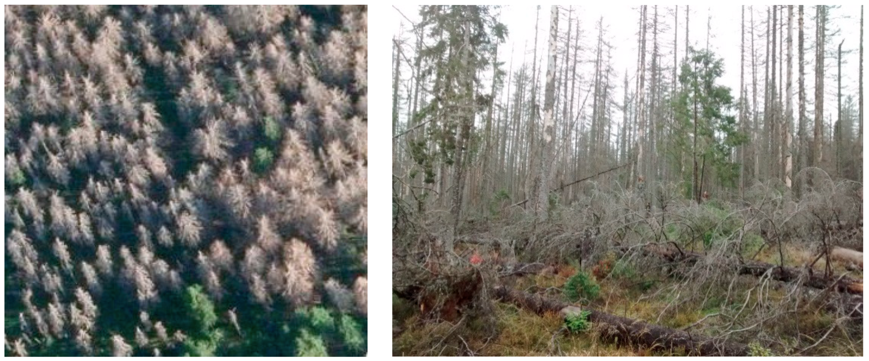
The dramatic die-off of spruce stands (Norway spruce, Picea abies (L.) Karst.) resulting from bark beetle Ips typhograpus outbreaks is a phenomenon experienced in many mountainous regions of Europe [14]. Both airborne [15] and satellite images (e.g., [16]) are used to evaluate forest stands after an insect attack. 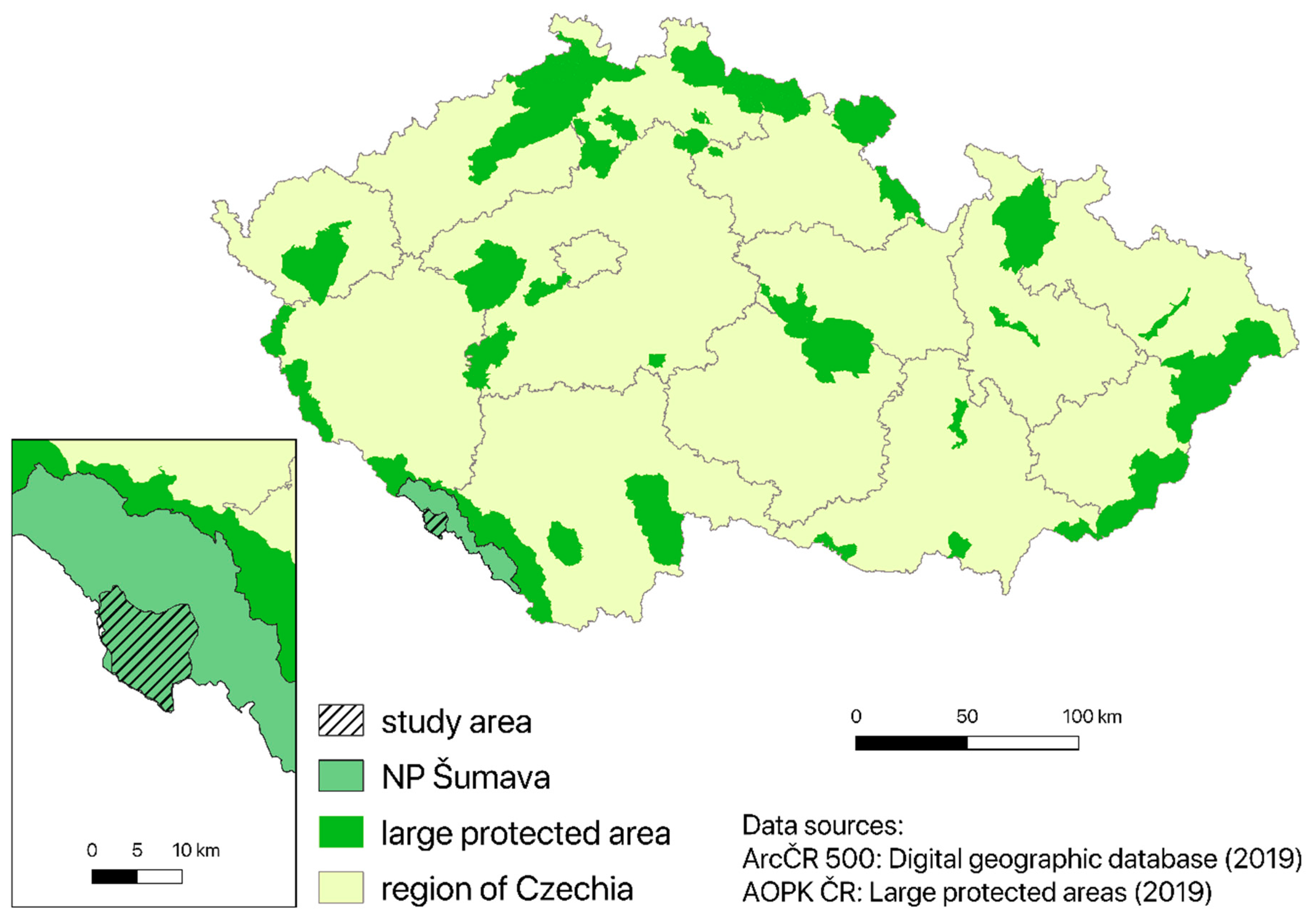An example of the use of WV2 is a work on the early detection of a bark beetle invasion in central Austria [12]. The researchers conducted a Random Forest classification determining the areas of forests that were healthy, under attack or dead. The Sumava National Park in Czechia has been struggling with long-term problems with disturbances, whether they be wind calamities or subsequent bark beetle invasions in Czechia. This national park, thanks to its overlap into the German Bavarian Forest, is very often examined by Czech authors [17,18,19,20] as well as foreign authors (e.g., [21]).

Choosing the appropriate classification method and defining a suitable definition of categories is an important aspect in assessing the condition and extent of the damaged forest. Many studies primarily focus on the pixel method used by Meddens et al. [15] or White et al. [22], who used it to detect a bark beetle red-attack. DeRose et al. [23] evaluated the affected forest with vegetation indexes from Landsat images, and the subsequent pixel classification achieved a total accuracy of 80–82%. Hicke and Logan [24] focused on the classification of 3 categories using the maximum probability classifier: healthy trees, damaged trees and grasslands. The study successfully separated the red attack trees from the healthy trees and the grasslands, thanks to the RGI (Red Green Index) index and the use of reflectivity in the green zone. The overall classification accuracy was 86%. In recent years, the area of state-of-the-art classifiers, such as Support Vector Machines (SVMs), Neural Networks (NNs) or Object-Based Classification (OBIA), has been intensively developed in connection with the development and availability of data with better spatial and spectral resolutions. Latifi et al. [25] used OBIA to classify Landsat images for an 11-year period in the Bavarian National Park to map the related forest mortality classes. The SVM method was successfully used by Hart and Veblen [26], who classified a bark beetle forest from satellite and aerial photographs.

The objective of our study was to evaluate the usefulness of very high spatial resolution images (1.84-m WV2) and high spatial resolution images (30-m Landsat 8) to identify bark beetle outbreaks from satellite data using advanced per-pixel methods based on machine learning methods. The main aims are based on the current topics discussed in the literature, which focus on testing the individual types of data and classification methods [27,28,29]. This study fills a gap that earlier studies have not handled: using WV2 in such a forest affected by bark beetle outbreaks. The long-term impact of the forest attack by the spruce bark beetle in the Sumava National Park offers an ideal opportunity to test different classification approaches and to assess the forest stand damage using remote sensing data of various spatial and spectral resolutions. The reason for comparing Landsat 8 (L8) and WV2 data was the unique timing of the acquisition of both types of data. Both images were acquired within one month in the autumn of 2015. The classification methods used are SVM and NN, which have been tested for input parameters, training areas, and other important parameters (e.g., number of iterations and background layers). The monitored categories are determined on the basis of field research, the suitability of the data inputs, a search for relevant studies and also the requirements of potential end users, such as hydrologists, foresters or management employees of the Sumava National Park. The next goal is to calculate the total area of the classified categories and to evaluate a spatial distribution of the categories in the case study. To recapitulate, the study deals with these goals:

• to evaluate and compare the applicability of the commercial, very high spatial resolution images (1.84-m WV2) with the freely downloaded, high spatial resolution images (30-m L8) for the identification of forest damage (affected by the bark beetle outbreaks);
• to compare the results of the classification of forest vegetation using the advanced classification algorithms of SVM and NN based on machine learning methods;
• to define the most relevant parameters of SVM and NN (e.g., number of iterations, background layers, kernel function, penalty parameter) for the highest accuracy to be achieved in the classification of land cover;
• to propose a classification system with definitions of categories to distinguish between the individual stages of decay and forest regeneration after a spruce bark beetle attack;
• to interpret the results of the classification and define the positives and weaknesses of the used data and classification methods.

2. Area of Interest

The area of interest in this study is the central part of the Sumava National Park, focusing on sites with a significant amount of decay of mountain spruce trees due to the overgrowth of the spruce bark beetle. The Sumava National Park, situated in the south to south-west of Czechia, is the largest national park in Czechia, established in 1991, and has a total area of 680 km². The surveyed area in the Sumava National Park copies the boundary of the provided WV2 image and covers 105 km² (see Figure 1).

The elevation in the area of interest reaches, on average, 1100–1200 m above sea level. The main landscape cover in the Sumava National Park is mountain spruce forests, peat bogs and mountain meadows. Most of the landscape has been influenced to a greater or lesser extent by the economic management of forests in the past, in particular by logging or livestock grazing. Although these activities lasted for a long time, we can still find scattered forest remains in the Sumava National Park [20]. The natural representation of spruce in the Sumava NP used to be around 51% but, during the last 250 years, the activity of spruce has gradually increased to about 80%. Spruce, thus, prevails in conditions where fir and beech trees prevailed in natural forests. In addition to spruce trees, there are many other specific plant and animal species in the Sumava NP; therefore, a special environmental protection regime has been established.

The core area of Sumava has been influenced by spruce bark beetle attacks for a long time. After 1990, the range of assaults began to rise mainly due to the recurring calamities and a series of dry and warm years that significantly reduced the forest’s resilience. The extremely dry and warm weather of 2003 was favorable for the development of the bark beetle and led to a re-weakening of spruce stands [3]. There was a large number of fallen trees that succumbed to the windstorm Kyril in January 2007. The fallen trees then became a suitable place for bark beetle attacks, and their populations increased radically [3]. The current state of the forest stands is strongly influenced by these calamities.

3. Materials and Methods

3.1. The Satellite Data Used

The first data source in our study is the multispectral images of WorldView-2, taken on 17 September 2015, under a cloudless sky. The acquisition of the WV2 data was finally successful in autumn 2015, since the first request for the acquisition of the WV2 data for Sumava was submitted in March 2013 to the official distributor of WV2 data. The resulting composite image was embedded in the UTM coordinate system (band 33) of the WGS-84 ellipsoid in the Ortho-Ready Standard (OR2A) version. WV2 offers a very high spatial resolution with 8 spectral bands. These 8 spectral bands are coastal, blue, green, yellow, red, red edge, 2 near infrared (NIR) bands. The spatial resolution is 46 cm for a panchromatic image and 1.84 m for a multispectral image (

Table 1. Spectral bands of WorldView-2.

Band	Name of Band	Range from (μm)	Range to (μm)
1	COASTAL	0.40	0.45
2	BLUE	0.45	0.51
3	GREEN	0.51	0.58
4	YELLOW	0.59	0.63
5	RED	0.63	0.69
6	RED EDGE	0.71	0.75
7	NIR 1	0.77	0.90
8	NIR 2	0.86	1.04

).

The second type of data used was Landsat 8 (L1TP) with a panchromatic spatial resolution of 15 m for multispectral images of 30 m. Landsat images, due to their availability since 1972 and their free distribution, are among the most widely used remote sensing data images for RS. For this reason, the Landsat data were used in order to compare them with the commercial data of WV2. The L8 image used was taken on 12 October 2015, i.e., less than one month after WV-2 acquisition. Landsat 8 OLI has 7 spectral bands, including 4 visible bands (coastal, blue, green and red), 1 NIR and 2 short-wave infrared bands (SWIR 1 and SWIR 2), see

Table 2. Spectral bands of Landsat 8.

Band	Name of Band	Range from (μm)	Range to (μm)
1	COASTAL	0.43	0.45
2	BLUE	0.45	0.51
3	GREEN	0.52	0.6
4	RED	0.63	0.68
5	NIR	0.85	0.89
6	SWIR 1	1.56	1.66
7	SWIR 2	2.1	2.3

.

3.2. Classification System

The area under investigation is of a very heterogeneous nature with a large number of different forest forms, whether bark beetle-affected or healthy. Prior to classifying the images, it was necessary to specify a classification system (legend) and define each class in detail. The designated definition of categories was based primarily on the literary sources [17,20] dealing with a similar theme, field research and the requirements of foresters and workers of the Sumava National Park. Above all, by using the Landsat multispectral data or WV2 with high spatial resolution, the effort was made to establish detailed definitions of categories depicting the individual species and health of the forest trees. A total of 9 categories were determined, of which 3 categories are non-forest, and 6 categories classify the forest vegetation. A detailed description of the categories is presented in Appendix A.

3.3. Data Preprocessing

3.3.1. Orthorectification

The provided WV2 data were supplied by the provider at the Ortho-Ready Standard (OR2A) level. The data were radiometrically and geometrically corrected. However, at the OR2A level, no correction for the topographic relief is performed. For this reason, the image had to be ortho-rectified before use. A method of rational polynomial functions was used. The principle of this method is the approximation of the orbital satellite model using multidimensional polynomial functions. The input parameter values are supplied together with the satellite data in the form of special metadata as Rational Polynomial Coefficients (RPCs). This method can be performed with or without a very small number of control points. Since the obtained data already contained an added coefficient file (* rpb), this method of ortho-rectification was performed in the ENVI software, where ortho-rectification can be performed by rational function coefficients directly for the WorldView sensor (RPC Orthorectification workflow). A digital terrain model is needed to perform the function. For the purpose of this study, the digital terrain model (DMR 5G) from the Czech Office for Surveying, Mapping and Cadastre was selected. The model is based on the data acquired by altimetry airborne laser scanning with an accuracy (mean height error) of 0.3 m [30].

3.3.2. The In-Situ Data

A field survey was carried out in the case study at a similar time to when both datasets were acquired. The field data collection took place from 8 to 9 October 2015, i.e., 21 days after the WV2 image was received. The control points for each type of forest cover/class were determined and tracked by a GPS (Global Position System). The points were collected using the Trimble Geoexplorer 6000 Geo XT GPS with an accuracy of ±0.5 m. For the purposes of accuracy assessment, 80 points were collected representing different types of forest. The land cover of the points, collected in the field, was defined based on the classification system (see Appendix A) and subsequently checked using a publicly available orthophoto acquired in 2015 (WMS orthophoto services). Only the points that clearly characterized the category were included.

3.3.3. Classification Methods

Per-pixel classification approaches were used for this study. As the name suggests, the basic image element entering the classification is the pixel, to which each decision rule applies. In this study, advanced classification algorithms of neural networks and support vectors were used [31]. Both algorithms are also controlled by non-parametric classifications, which means that there is no presumption of a normal data distribution. This fact is the biggest advantage of the given classifications [32]. One of the basic principles of SVM is the conversion of the input space into multidimensional space, where the classes can be separated from each other linearly. The SVM algorithm seeks to find the optimal hyperplane that separates the data into a predefined number of classes according to the training set [33]. In essence, the SVM is a binary classifier, but there are procedures by which a method can be adapted to query multiple classes. We call these two approaches one versus one and one versus all [31,34].

The use of the Support Vector Machine classifier includes not only a suitable selection of the training set but also a selection of suitable parameters entering the classification. In the ENVI software, it is possible to select the type of kernel function (linear, radial basis function-RBF, sigmoid and polynomial), and it is also possible to set the γ value of the parameter (for the linear and RBF functions), the penalty parameter and the threshold value. The parameters chosen for the process in this work (see

Table 3. Applied support vector machine (SVM) parameters for Landsat 8 (L8) and WorldView-2 (WV2) images.

Combination	Kernel Function	Gamma Parameter	Penalty Parameter	Threshold	Polynomy
1	RBF	10	50	0	-
2	RBF	Default 1	90	0	-
3	RBF	Default 1	100	0	-
4	polynomial	Default 1	90	0	6
5	polynomial	Default 1	100	0	6

¹ Default value—snapshot Landsat 8, γ = 0.143, snapshot WorldView-2, γ = 0.125.

) are mainly based on our own testing as well as combinations used in previous studies, e.g., [35].

Neural networks represent algorithms that try to mimic processes occurring in the nervous system, where a network of specialized neural cells, neurons, processes the signal and converts it into information [32]. The neural network classification method forms a layer of neurons according to the input spectral bands that enter it. The output layer then consists of neurons, each of which is one of the classified classes. The neural network classification uses the back-propagation algorithm for training. The ENVI program [36], where the classification was conducted, allows one to select the following parameters that can influence the outcome and neural networking process: Training Threshold Contribution (TTC), Training Rate (TR), and Training Momentum (TM).

The parameters in question greatly influence the behavior of the entire process, so sufficient attention has been paid to their selection. The parameters chosen for the processing of data in this work (see

Table 4. Applied neural network (NN) parameters to L8 and WV2 images.

Combination	Training Threshold Contribution (TTC)	Training Rate (TR)	Training Momentum ™	Iterations	Number of Background Layers
1	0.2	0.2	0.4	1000	1
2	0.3	0.2	0.5	1000	1
3	0.1	0.2	0.5	1000	1
4	0.2	0.2	0.4	5000	1
5	0.3	0.2	0.5	5000	1

) are mainly based on our own testing as well as inspired by a study carried out in 2012 using SPOT data [37]. Testing the values of iterations and the TTC parameter was the most significant point for the definition of the combinations used in this study.

All the spectral bands of WV2 and L8 OLI, except coastal and panchromatic, entered the classification. So, a wide multispectral potential was used for both datasets: visible bands, NIR bands, the red edge of WV2 and the SWIR of L8. The coastal band is useful for imaging shallow water and tracking fine atmospheric/aerosol particles like dust and smoke [2] so is not a relevant band for the purpose of this study. The training set for the classification was collected using the orthophoto. The selection of points was then also verified using vegetation indices and combinations of spectral bands of satellite images (mainly using WV2). Representative points were found for each class of the classification. The number of training points for each class ranged from 11 (for the classes of C2, E and F) to 27 for the class of dead forest (see

Table 5. Training and control points.

Class	A1	A2	A3	A4	B	C1	C2	E	F	Total
Number of Training Points	25	24	20	27	16	23	11	11	11	168
Number of Control Points	20	16	12	17	10	15	6	7	6	109

Note: The points of water bodies (Category E) were excluded from the accuracy assessment of the Landsat classification because the water bodies were not classified by Landsat (low spatial resolution of Landsat).

and Appendix J).

Due to the very heterogeneous character of the landscape, the resulting classification using WV2 images manifested the so-called salt and pepper effect with a high number of isolated pixels. For this reason, a filtering was applicated on WV2 classification because of its suppression of the salt and pepper effect. After testing the individual filter methods, the median filter with a 5 × 5 grid was used.

3.3.4. Accuracy Assessment and Result Presentation

Classification accuracy was assessed based on error matrices (overall accuracy, producer accuracy, user accuracy and the Kappa index). The accuracy of the classifications was evaluated using the points collected in the field, which can be used in the SW ENVI 4.7 for Ground Truth ROIs. Field measurements were focused on the forest categories (healthy forest, affected forest, regenerating forest, dead forest and clear-cut forest). The categories of wetlands, permanent grasslands, water bodies and artificial surfaces were generated over the orthophoto and WV2 data using a visual interpretation. So, 80 points were collected by in-situ collection and 29 points by visual interpretation of the orthophoto and WV2 data. For the number of points for all the classes, see Table 5 and Appendix B, Appendix C and Appendix J.

Finally, the total area of the individual classes and the ratio of the class area to the total area of the case study were calculated, and a spatial distribution of the classification classes was evaluated using a comparison of the classification maps.

4. Results

In this chapter, the results of the WV2 and L8 multispectral image classifications are described and compared. The classification was performed using the SWM and NN algorithms to define the parameters for the most accurate results.

4.1. Evaluating the Accuracy of Classifications

The overall classification accuracy and the calculated Kappa index for each parameter combination are given in

Table 6. Overall accuracy and Kappa index classification of SVMs.

SVM	Parameters				WorldView-2		Landsat 8
Combination	Kernel Function	Gamma Parameter	Penalty Parameter	Polyonomy	Overall Accuracy (%)	Kappa Index	Overall Accuracy (%)	Kappa Index
1	RBF	10	50	-	76.15	0.73	68.63	0.64
2	RBF	Default 1	90	-	84.40	0.82	69.61	0.65
3	RBF	Default 1	100	-	84.40	0.82	70.59	0.66
4	polynomial	Default 1	90	6	84.40	0.82	70.59	0.66
5	polynomial	Default 1	100	6	86.24	0.84	70.59	0.66

¹ Default Value—Landsat 8, γ = 0.143, WorldView-2, γ = 0.125.

and

Table 7. Overall accuracy and Kappa index classification of NNs.

NN	Parameters				WorldView-2		Landsat 8
Combination	Training Threshold Contribution	Training Rate	Training Momentum	Iteration	Overall Accuracy (%)	Kappa Index	Overall Accuracy (%)	Kappa Index
1	0.2	0.2	0.4	1000	80.73	0.78	67.65	0.63
2	0.3	0.2	0.5	1000	81.65	0.79	68.63	0.64
3	0.1	0.2	0.5	1000	81.65	0.79	69.61	0.65
4	0.2	0.2	0.4	5000	81.65	0.79	64.71	0.59
5	0.3	0.2	0.5	5000	78.90	0.76	65.69	0.60

.

The overall SVM classification accuracy varies between 76.15% and 86.24% for WV2 and between 68.63% and 70.59% for L8 according to the selected parameter combination. As we can see, the best results were achieved using Combination 5, where a polynomial function was applied. The worst results are shown in Combination 1, where the gamma parameter and the parameter penalty have been significantly adjusted for the RBF function. If we compare the accuracy of the satellite data used, the accuracy is higher in the WV2 image than in the L8 image.

If we compare the results of the SVM algorithm with the NN algorithm (Table 6 and Table 7), we can see that the overall accuracy values of NN are generally 2.5% lower on average. For both images, the highest overall accuracy and Kappa index were achieved when Combination 3 was selected. Very similar overall accuracy values were achieved by both the images of WV2 and Combinations 2 and 4, respectively. As can be seen, despite the increase in the number of iterations, there was no improvement in the results and, thus, no higher accuracy. Conversely, in Combination 5, WV2 has the overall lowest accuracy.

It is clear from the results of the classification that categories A1–4 are the worst separable classes (see Appendix B and Appendix C). The A2 class of forest was, in many cases, confused with the category of dead forest A4. This fact is, of course, associated with a very wide (fuzzy) boundary between the two classes, mainly in terms of class definition (spectral characteristics, see Appendix I). The best user accuracy results for the A3 category were achieved by the SVM method applied to the WV2 image. For the category of regenerating forest A3, classes A1, A4 and C1 or C2 were most commonly confused. SVM and NN classifications based on WV2 distinguished class B with nearly 100% accuracy. On the other hand, a lower accuracy was achieved using the L8 image.

4.2. Comparison of the Area and Spatial Distribution of the Classification Classes

The relative representation of classes is given by the ratio of the class area to the total area of the classified area. The percentages of the representation of the individual land cover classes of the resulting WV2 image classifications are shown in Figure 2. As we can see in this figure, the biggest differences between the classification results can be found in categories A2, A3, A4 and C1. Both the A1 and A2 categories are similar in both classifications SVM and NN. Class A3 is about 6% lower in the SVM than the NN. However, at the expense of this category, the area of forestry clearings and openings C1 is increased. For the SVM and NN algorithms, we see that category E is highly overestimated. This fact can be explained by the numerous shadows in the image that were included in the water surface.

When comparing the resulting areas for L8 and WV2 data (see Figure 2 and Appendix D, Appendix E, Appendix F, Appendix G and Appendix H), it is evident that the largest area on the classified data is occupied by the category A3, and the smallest area by C2 and F. There is a high variation in the size of class B. The area of category B is almost doubled on the classified L8 images compared to the WV2 ones. This phenomenon is probably due to the specificity of this category, which does not reach large areas, and could be defined by the data with a high spatial resolution. The Landsat data with a lower spatial resolution could not accurately detect this category. As a result, the relative area of category A1, A2, or A4, which is mostly in the vicinity of class B, is dropped and part of its area is assigned to this class. The strong drought phenomenon also played a role, with category B (normally occurring soil moisture) in the images having almost identical spectral characteristics to category A1 and A3.

5. Discussion

The main aim of the study was to evaluate the possibilities for the classification of forest stands affected by disturbances in the Sumava National Park. For this purpose, WV2 and L8 satellite images taken at a very similar time in 2015 were selected and compared. The next goal was to evaluate and compare the results of SVM and NN classifications based on the input satellite data.

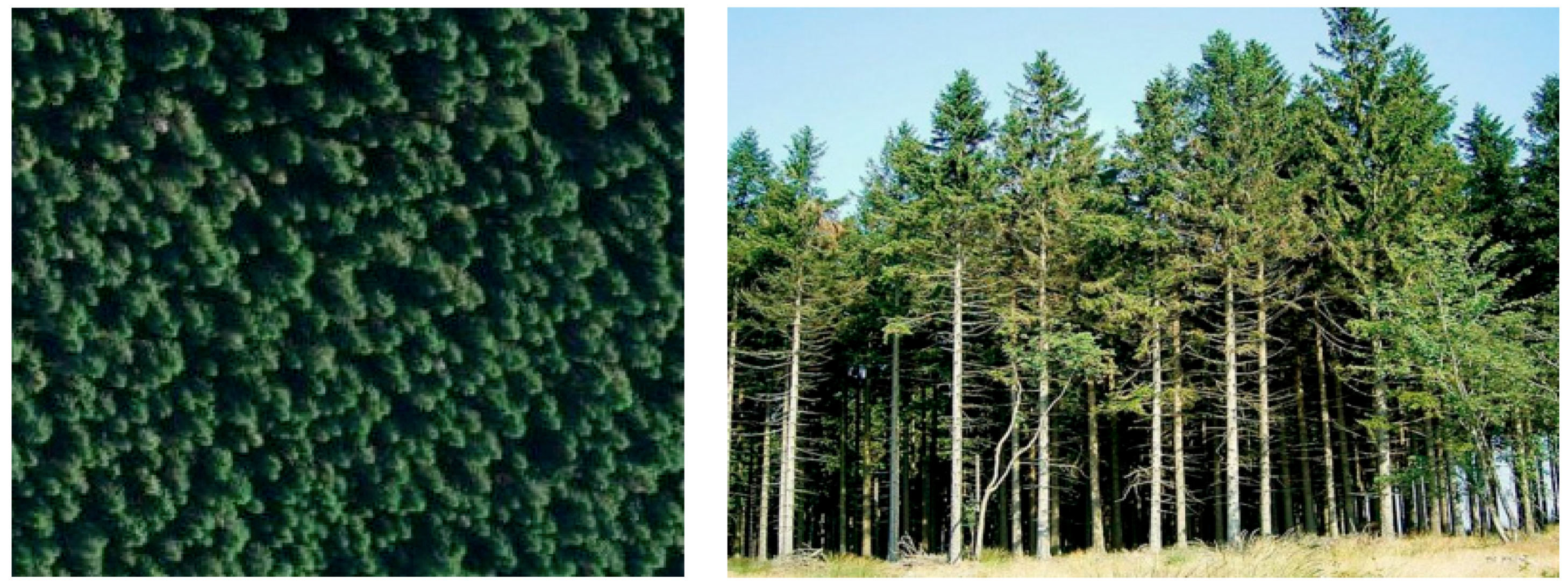
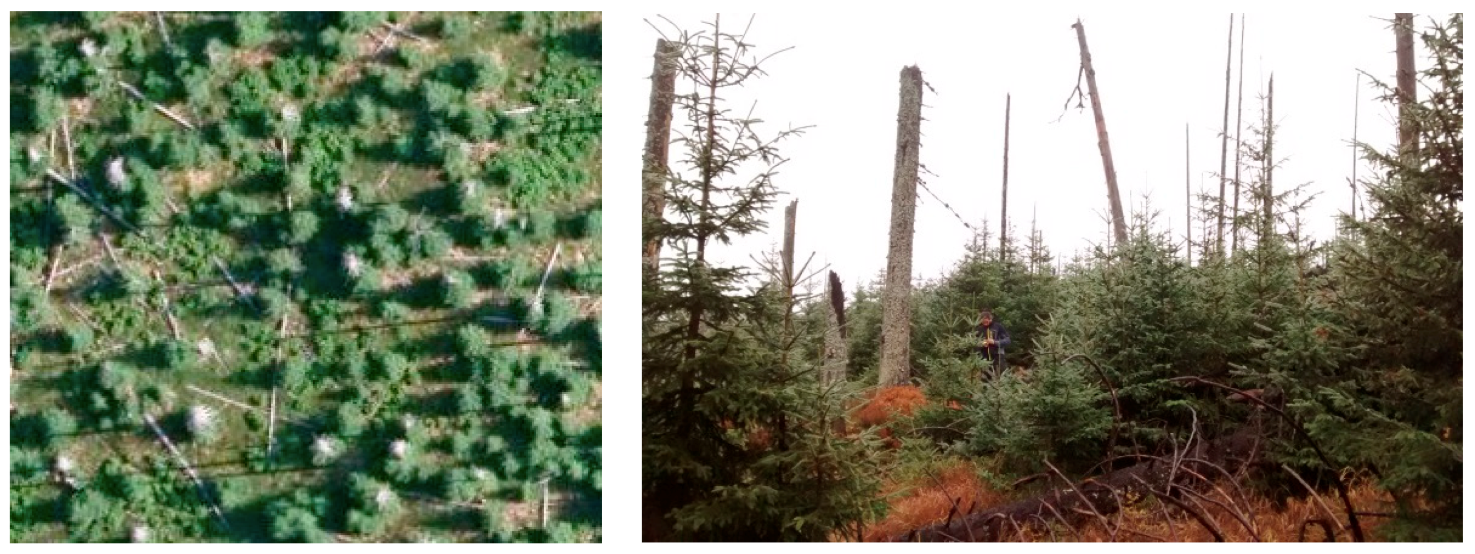
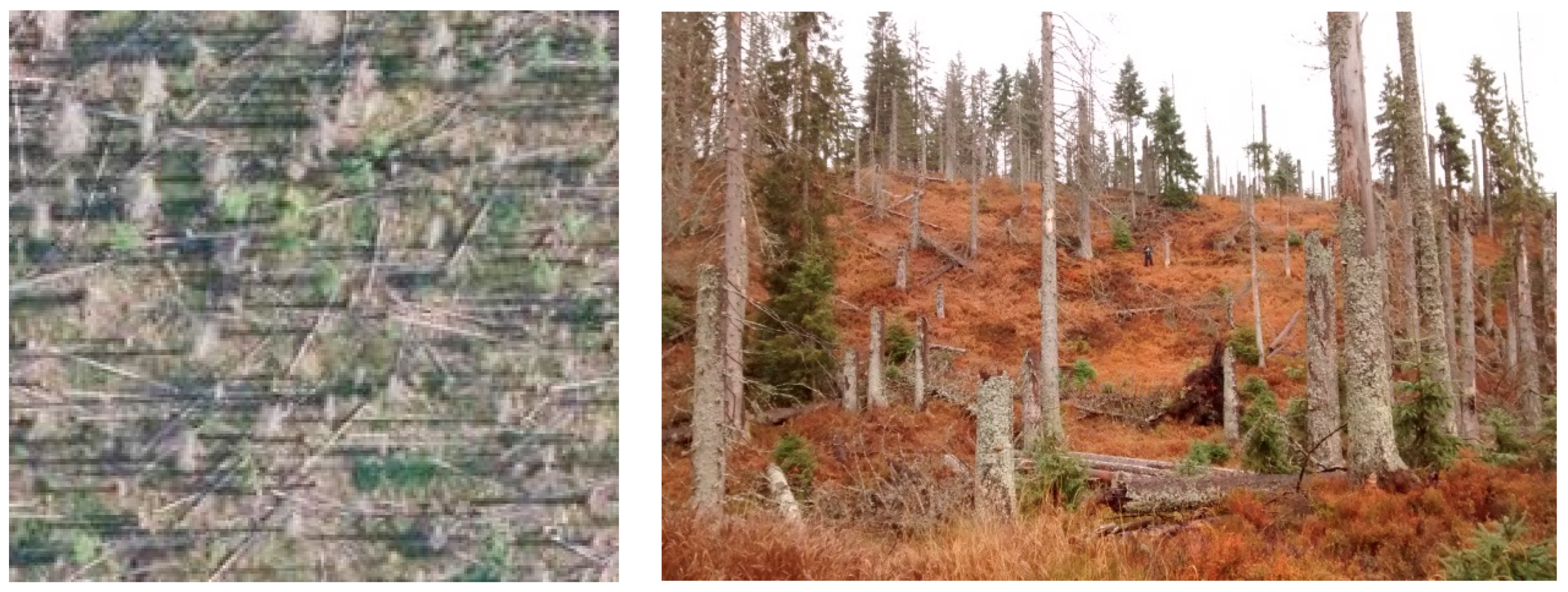
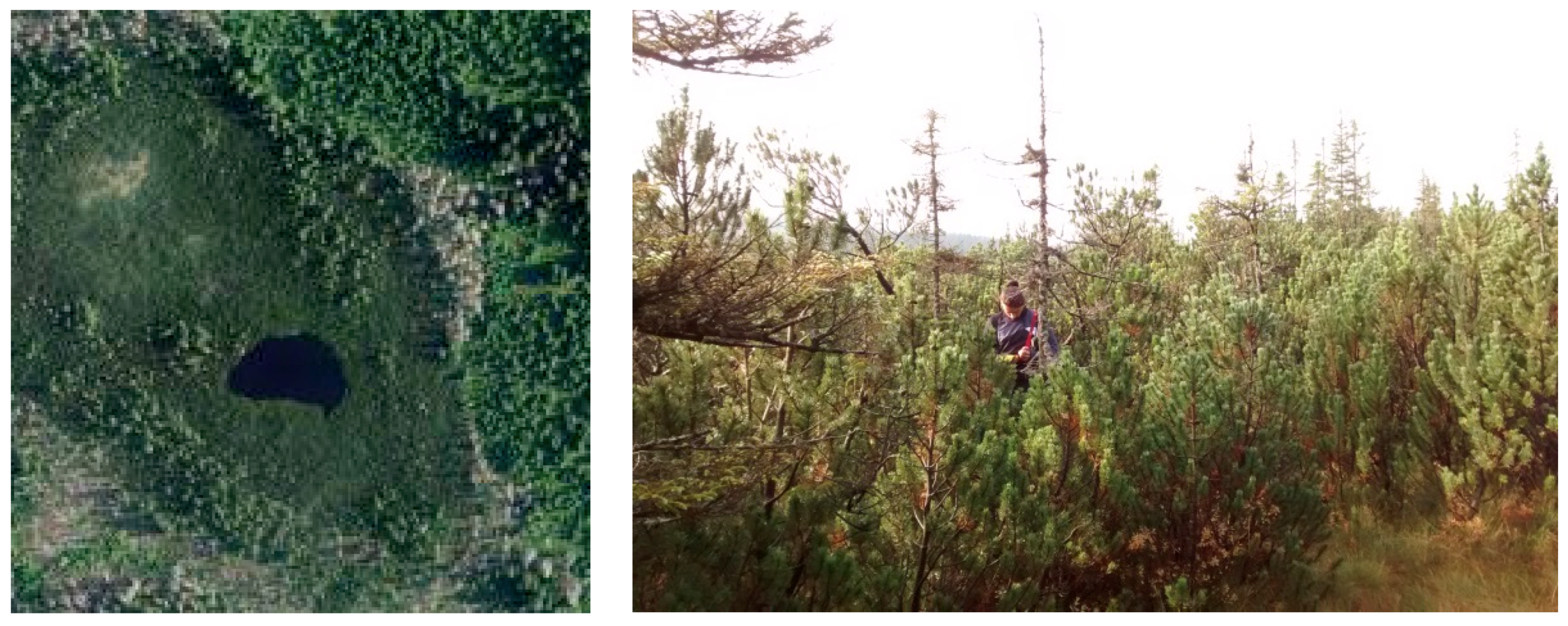
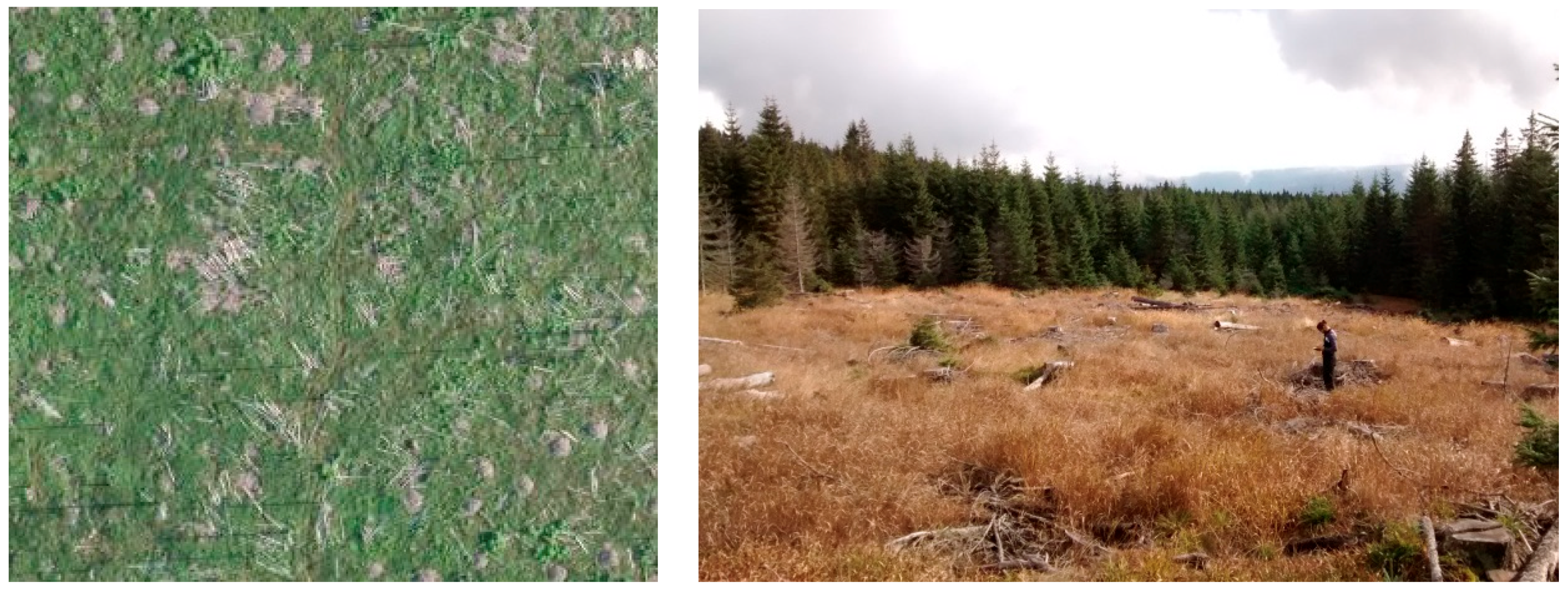
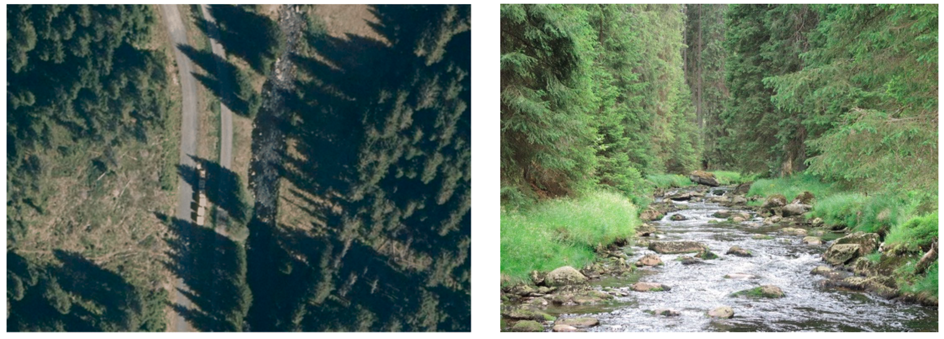
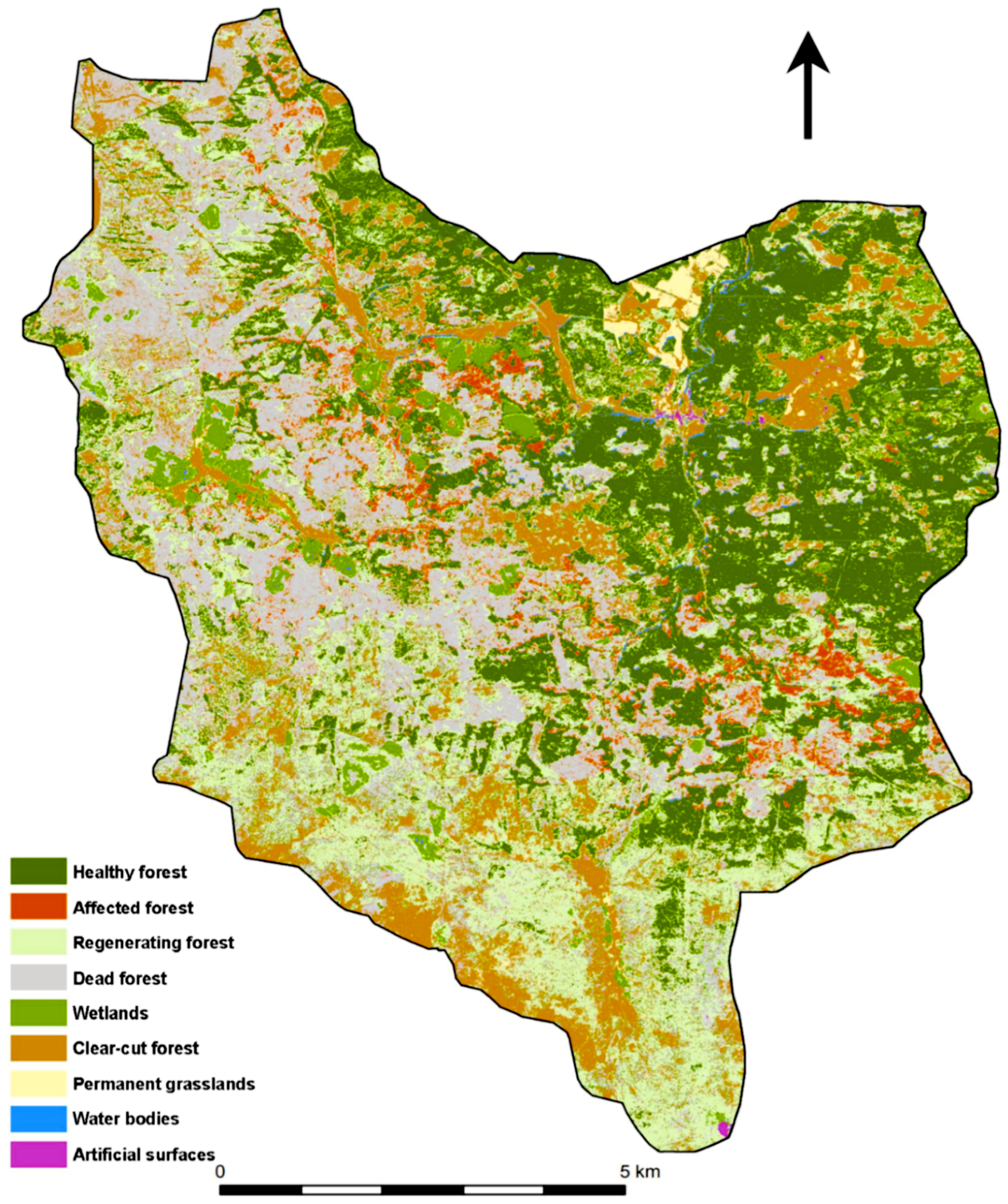
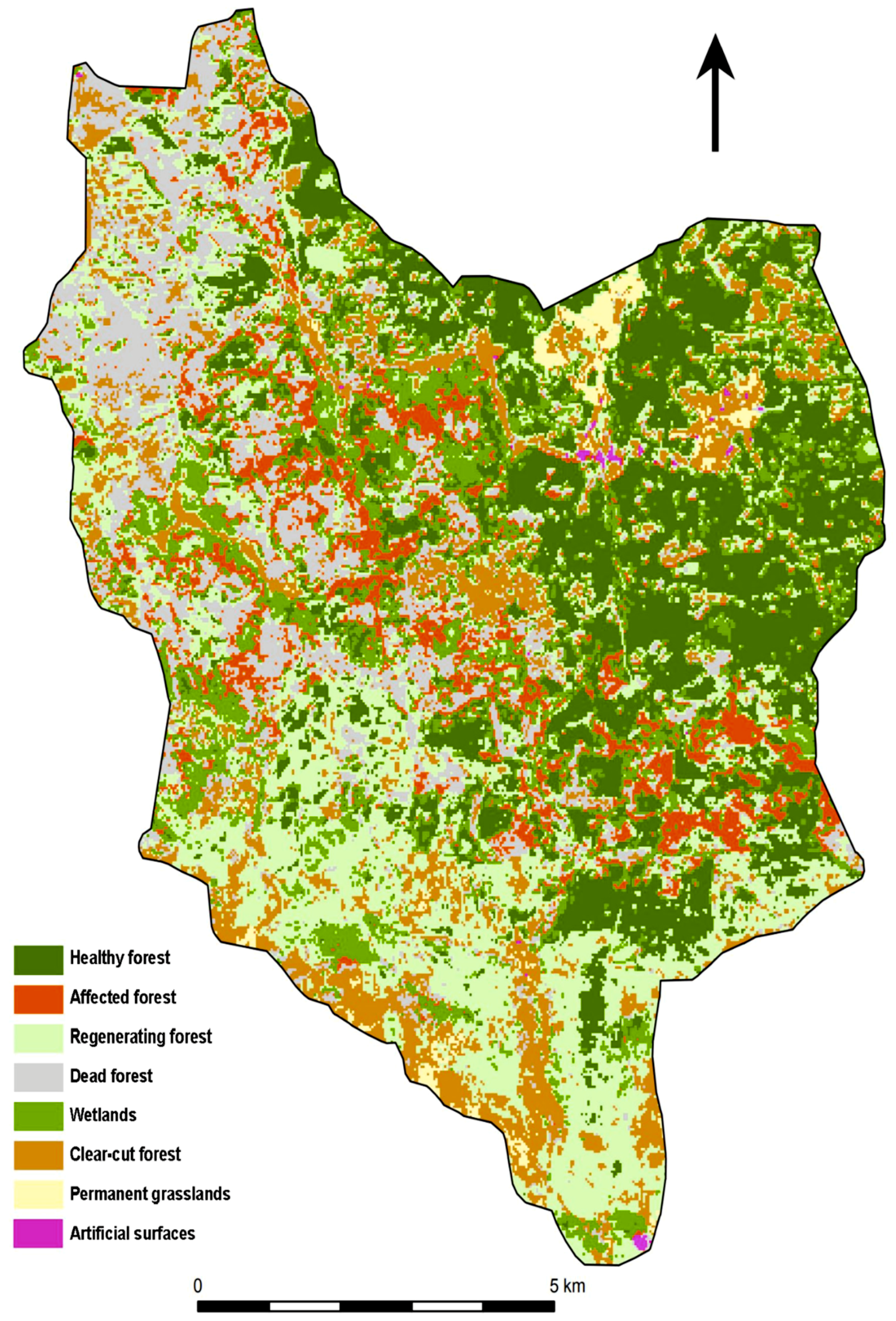
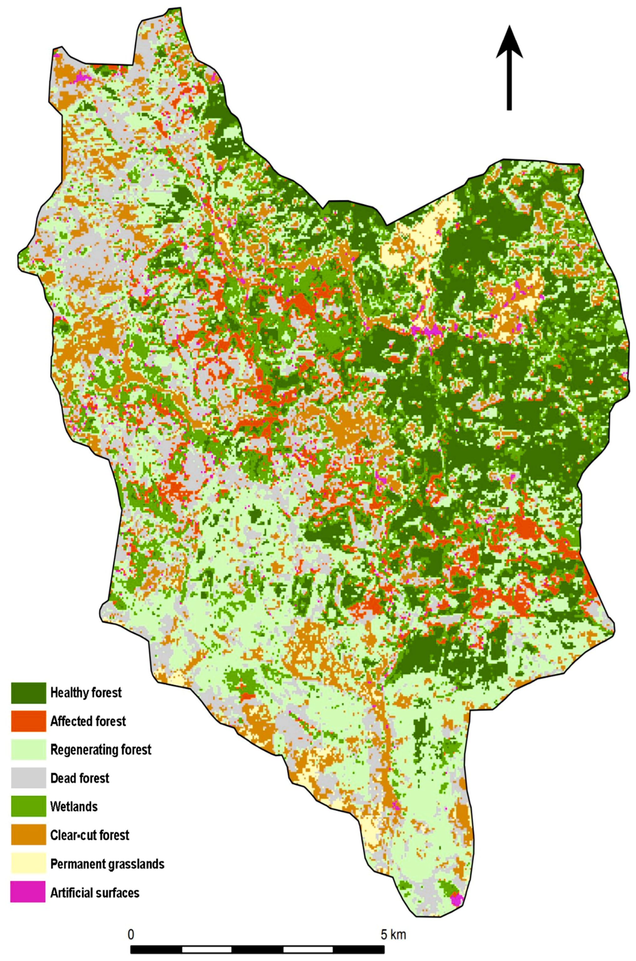
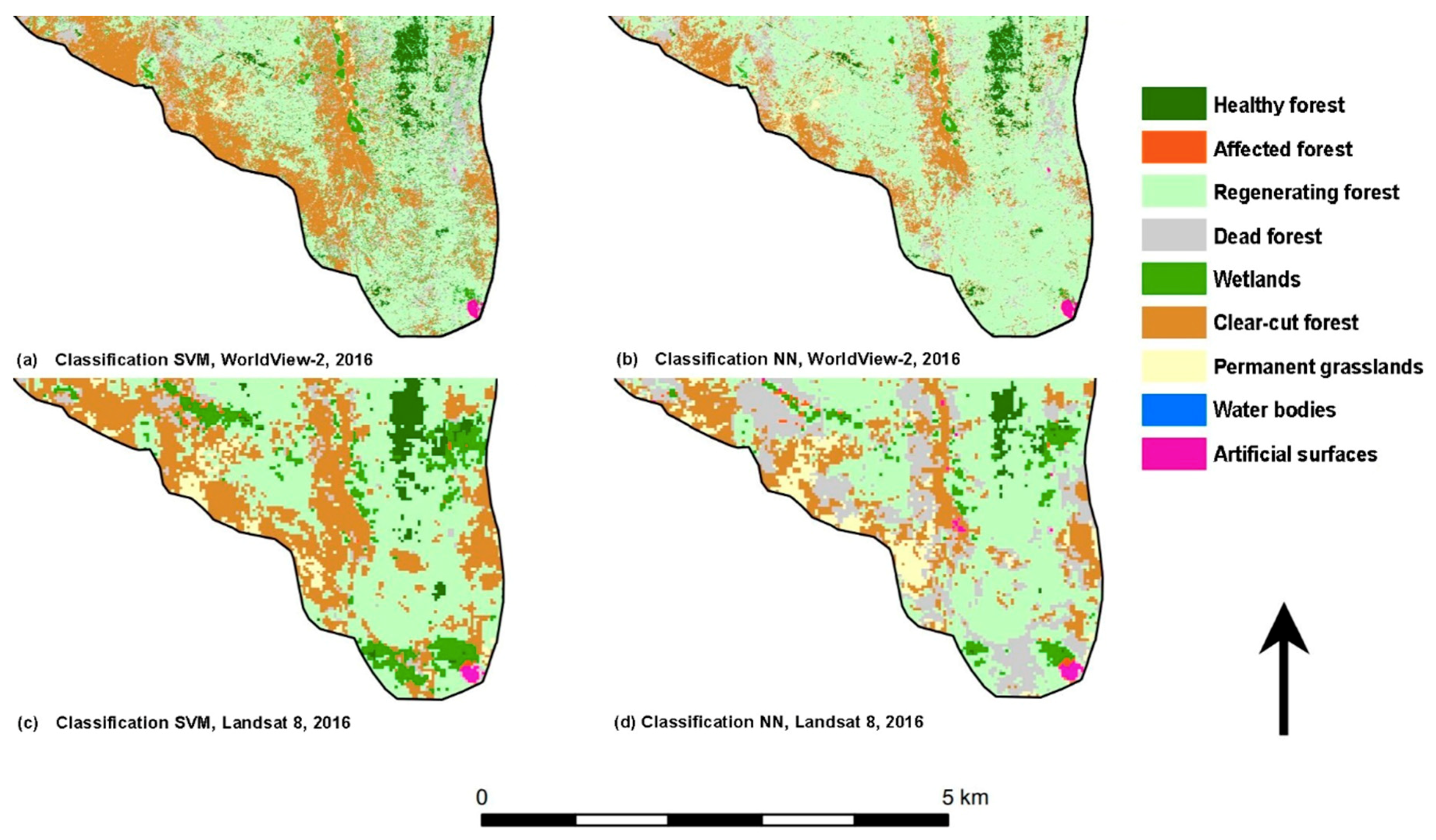
The resulting classification is based on a definition of categories that was primarily designed to distinguish between the observed stages of decay and forest regeneration after the spruce bark beetle attack. The classification classes, thus, reflect the state of vegetation in the Sumava National Park in 2015, and their definition is based on findings from a field survey, results of similar studies and experts from the Sumava National Park. The forest stands were divided into the following categories: A healthy forest, an affected forest, a dead forest, a regenerating forest and a clear-cut forest. This distinction is important from an environmental point of view, from the perspective of decision-making processes in forestry, and in nature and landscape protection. The most important aspect in determining the classes was the purpose of using the classification outputs. In the case of this study, the requirements of foresters and conservationists for forest stand monitoring and the requirements of physical geographers and hydrologists were accepted.

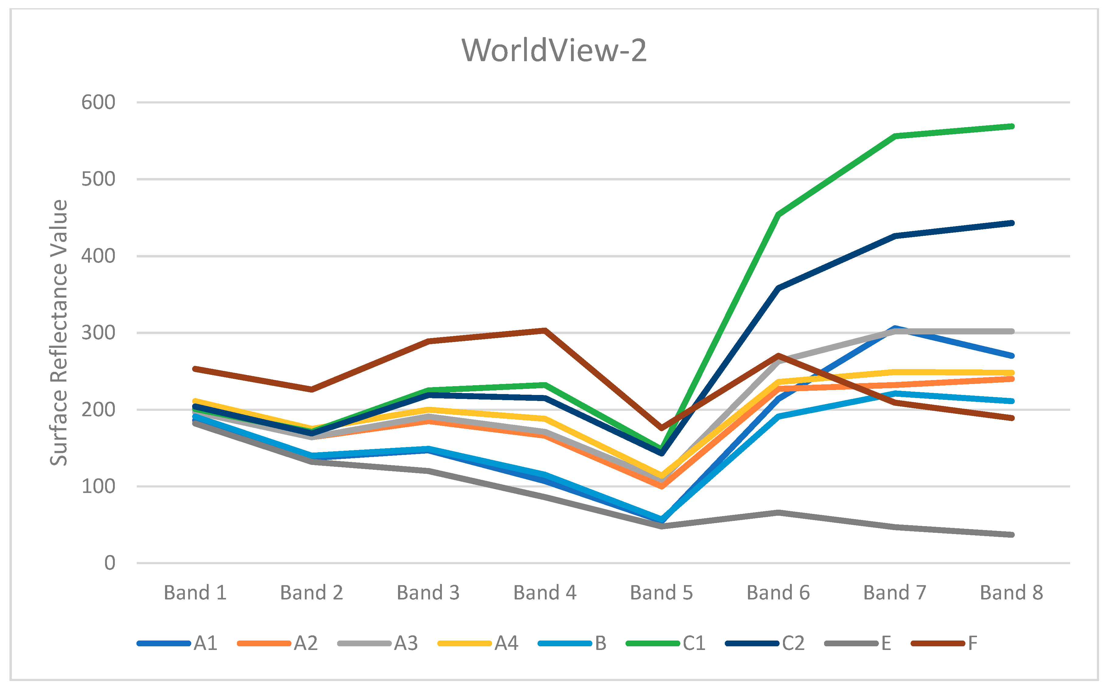
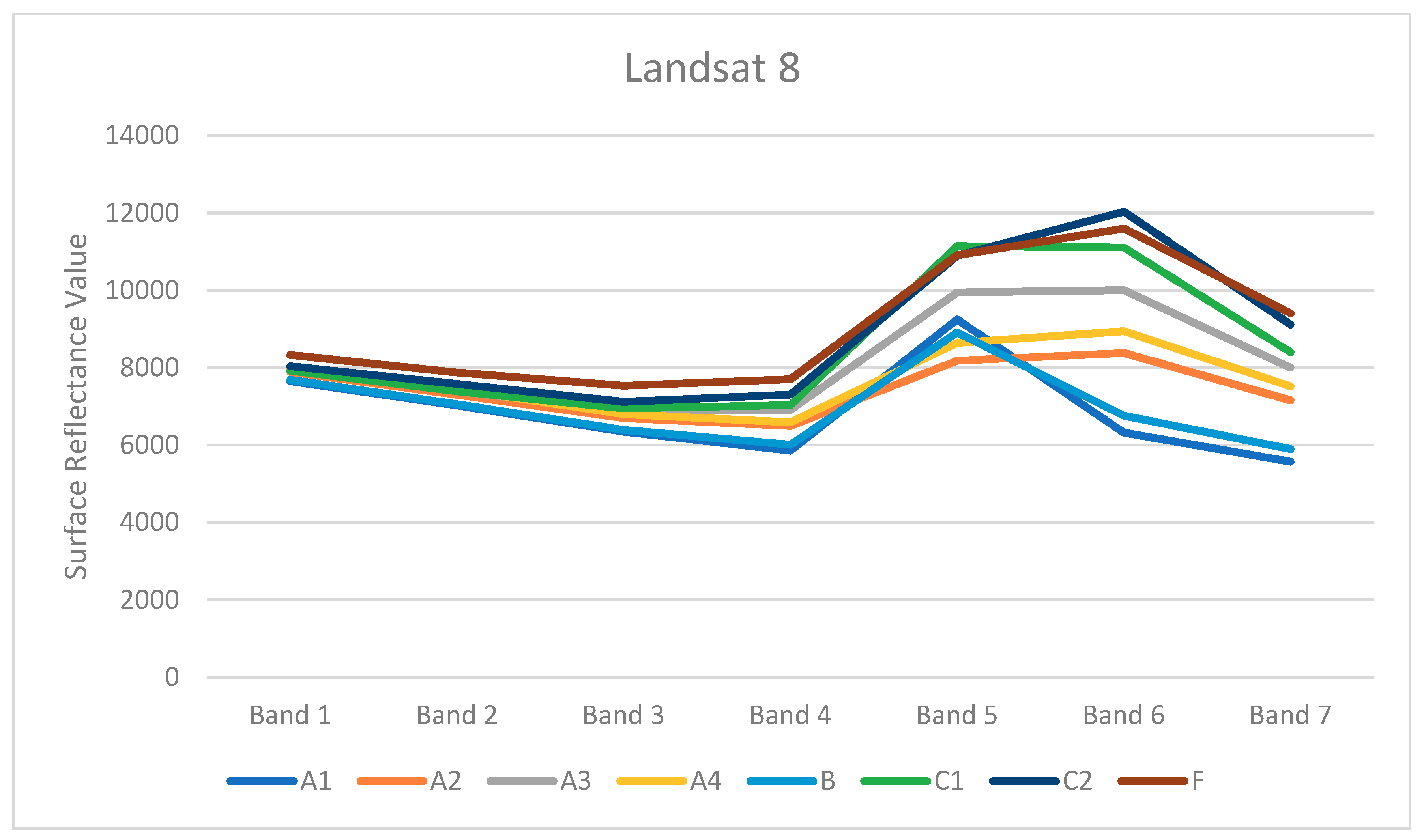
This study proved a high potential of the multispectral satellite data for research on forest vegetation affected by bark beetle outbreaks. Near infrared (NIR) and short-wave infrared (SWIR) bands are crucial for distinguishing the individual forest categories and for the evaluation of the health of forest vegetation [1,17]. From the point of view of evaluating the accuracy of the classification of individual classes, a problematic classification was assumed for the classes of the affected (A2), dead (A4) and regenerating forest (A3). In these classes, the spectral characteristics may be similar, making it more likely to be confused among themselves or, for example, with the category of clear-cut forest (C1). This assumption was confirmed; however, the classification of WV2, which has a higher spatial resolution, brought better results than L8. Most precisely, these categories were distinguished by the SMV classification based on WV2, see the error matrix tables in Appendix B. Besides, due to the small area/size of local water bodies, it was not possible to classify these areas with respect to the Landsat 30 × 30 m spatial resolution. When classifying a Landsat image with a lower spatial resolution, the water bodies class could not be classified. From the point of view of the classification, negatives of higher resolution data are shadows, which are more visible in the WV2 image.

For the classification methods, the SVM and NN methods were selected for classification based on previous studies that dealt with forest classification, e.g., [9,15,37]. These methods were applied to the WV2 and L8 satellite imageries (commercially × freely downloaded date). After evaluating all the available results, the SVM can be considered a better method than NN. This classifier achieved the highest overall accuracy and Kappa index for both classified images. In the case of WV2 and L8, total overall accuracies of 86% and 71% and Kappa indices of 0.84 and 0.66 were achieved with SVM, respectively. The NN algorithm using WV2 also produced very promising results, with over 80% overall accuracy and a Kappa index of 0.79. Due to the very heterogenic character of the forest in the case study, the achieved accuracy could be considered as acceptable, although some previous studies e.g., [24] achieved a higher accuracy. However, these studies did not focus on such damaged and heterogenic forests.

The testing of the appropriate parameters for the classification of both algorithms became an important step. The choice of the parameters for the SVM and NN classifiers was based primarily on our own testing and the studies already carried out to address a similar topic in the given area. Some of the results reported [37] were confirmed in this study based on different data, especially, the fact that accelerating the process of training the NN network does not lead to better results. The highest accuracy of NN brought the adjustment of the Training Threshold Contribution to 0.1 and 1000 Iterations. In the SVM algorithm, the choice of values for the parameters offered was mainly influenced by the selected Kernel function. RBF and polynomial functions were selected for testing. The polynomial function provided a better accuracy than RBF. After evaluating all the available results, SVM can be considered as a better method than NN. This classifier achieved the highest overall accuracy and Kappa index for both classified images. Similarly, in the case of the most important classes from the perspective of forest growth (forest management) A1–4, using SVM, the best results were achieved for both the user and the processing accuracy. The NN algorithm of WV2 also produced very good results, with over 80% overall accuracy. In the L8 image, the effect of the lower spatial resolution in class B and F classifications is evident.

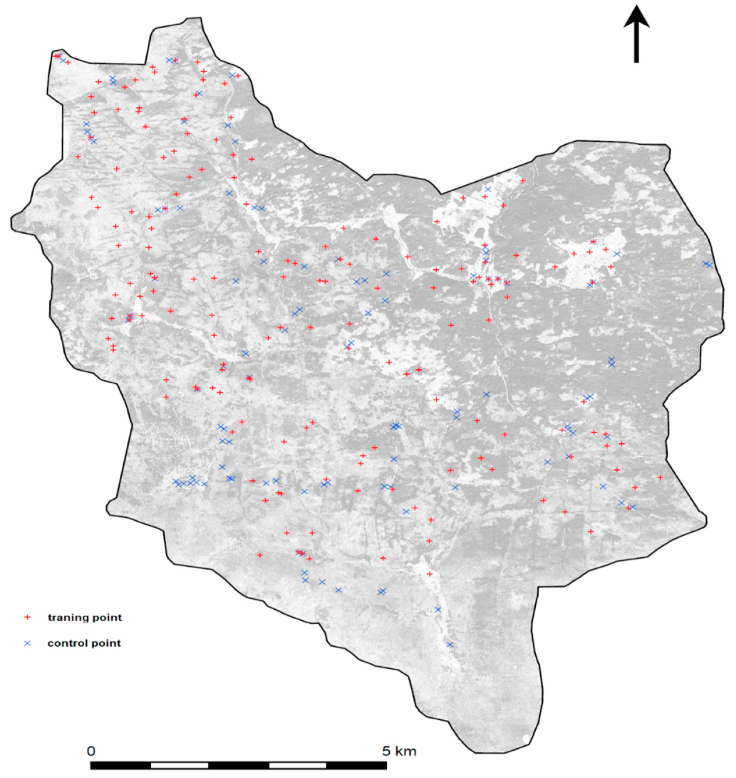
An important part of the classification is certainly the creation of a training set and control points. It is essential that the training points for each class are evenly spatially distributed. At the same time, it is also necessary that the control points of the classification are measured at the similar time as the acquisition [32]. In the case of this work, the control points of the forest categories were collected several days after the acquisition of the WV2 data. The calculation of the accuracy of the classifications was based on the control points that were measured using a GPS device (80 points were measured in the forest vegetation). These points were supplemented by the points derived from the orthophoto and WV2 multispectral data, e.g., water bodies, artificial areas. The final number of checkpoints was 109 points for WV2 and 102 for Landsat 8. In order to verify the results of this study, it would be useful to consider collecting more control points in the future, especially for forest stands.

The disadvantage of pixel classification is the so-called salt and pepper effect. For some suppression of this effect, a median filter with a 5 × 5 grid was used. However, this method did not remove all the small areas (single pixels), and its implications could influence the resulting scores in the accuracy assessment and the comparison of L8 and WV2 images. This is one of the great advantages of the OBIA object classification, where it is not necessary to solve the problem of single pixels thanks to the initial segmentation.

Comparing the results of the classification and accuracy assessment of the WW2 and L8 images, the effect of the better spatial resolution is evident for the WV2 image. The SVM classification of this image achieved better accuracy for the forest classes (A1–4) as well as the other classes than the classification based on L8. In particular, the forest categories (healthy, affected, regenerating and dead forests) are very relevant from the ecological and forest management point of view, so the ability of WV2 to separate these categories is very significant. A combination of the very high spatial resolution and the suitable spectral resolution, with 8 visible and near infrared bands in the WV2 image, seems to be crucial for the classification of the forest categories affected by disturbances. On the other hand, the archive of Landsat data is free and provides a long-time series of data (since the 1970s). So, it is possible to analyze L8 data using time series methods and to investigate changes in forests based on the multitemporal data of L8.

Based on the results of our case study, it was confirmed that WV2 data had better abilities in the classification of disturbed forest than L8 data. WV2 is useful in small-scale case studies due to the better spatial resolution with a suitable spectral resolution (visible, red edge and NIR bands) see [12,13]. According to the results of many studies [9,11,17], Landsat data are suitable for large-scale case studies/regions. Landsat data also enable the evaluation of changes in the forest vegetation over a long-term period. In general, the most important factors for an evaluation of the data used in a classification are the purposes and objectives of the study (classification system, scale, requirements of the end-users etc.). Obviously, WV2 data were more significant and useful than L8 for the purposes of this study.

With regard to the application of the classification methods to the Sumava National Park, it is not possible to say with certainty whether similar results would be achieved in other territories. In order to generalize the presented conclusions, it would be necessary to test the whole procedure on more than one area of interest. The best transferable method could be the SVM algorithm, which requires an appropriate training set, and within which it is relatively easy to define input parameters. NN methods, meanwhile, require more experience of the processor especially in terms of detailed knowledge of data and territory. Anyway, it would be useful to test other combinations of parameters with the classification methods in different case studies. An evaluation of vegetation indices as input data in classification could be another way of investigating this thematic in depth.

As for testing other types of data, it would undoubtedly be useful to include Sentinel-2 or Planet.com data (PlanetScope, SkySat) in the testing. The availability of new types of data since 2015, when the data used for this study were collected, has increased dramatically. So, this study can be taken as an inspiration for future studies that will use more modern data types or different classification algorithms such as the Random Forest Classifier.

6. Conclusions

The objective of this paper was to assess the WorldView-2 and Landsat 8 images along with the Support Vector Machine and a Neural Network classifier in the detection of bark beetle outbreaks in the Sumava National Park. Based on the accuracy assessment and achieved results, the Support Vector Machine can be considered as a more suitable method than the Neural Network. The most relevant parameter leading to the highest accuracy is the Kernel function in the SVM algorithm. The polynomial of the Kernel function provided a better accuracy than RBF. The classification system used was primarily designed to distinguish between the observed stages of decay and forest regeneration after a spruce bark beetle attack. This distinction is important from an environmental point of view, from the perspective of decision-making processes in forestry and nature and landscape protection. The methods used in this study may be inspirational for testing other types of satellite data (e.g., Sentinel-2) or other classification algorithms in different case studies.

References

1. Jensen, J.R. Remote Sensing of the Environment: An Earth Resource Perspective, 2nd ed.; Pearson Prentice Hall: Upper Saddle River, NJ, USA, 2007. [Google Scholar]
2. Zhu, Z.; Woodcock, C.E. Continuous change detection and classification of land cover using all available Landsat data. Remote Sens. Environ. 2014, 144, 152–171. [Google Scholar] [CrossRef] [Green Version]
3. Hais, M. Využití dálkového průzkumu země pro monitoring lesů na Šumavě. Životní Prostředí 2009, 4, 216–219. [Google Scholar]
4. Kupková, L.; Potůčková, M.; Lhotáková, Z.; Albrechtová, J. Forest cover and disturbance changes, and their driving forces: A case study in the Ore Moutains, Czechia, heavily affected by anthropogenic acidic pollution in the second half of the 20th century. Environ. Res. Lett. 2018, 13. [Google Scholar] [CrossRef]
5. Tomppo, E.; Olsson, H.; Ståhl, G.; Nilsson, M.; Hagner, O.; Katila, M. Combining national forest inventory field plots and remote sensing data for forest databases. Remote Sens. Environ. 2008, 112, 1982–1999. [Google Scholar] [CrossRef]
6. Hostert, P.; Grogan, K.; Pflugmacher, D.; Jan, V.; Fensholt, R. Mapping Clearances in Tropical Dry Forests Using Breakpoints, Trend, and Seasonal Components from MODIS Time Series: Does Forest Type Matter? Remote Sens. 2016, 8, 657. [Google Scholar] [CrossRef]
7. Tuček, J. Príspevok k Hodnoteniu Zdravotného Stavu Lesov na Základe Rôznych Materiálov DPZ; Acta Facultatis Forestalis: Zvolen, Slovakia, 2001; pp. 341–354. [Google Scholar]
8. Kozak, J.; Estreguil, C.; Troll, M. Forest cover changes in the northern Carpathians in the 20th century: A slow transition. J. Land Use Sci. 2007, 2, 127–146. [Google Scholar] [CrossRef]
9. Griffiths, P.; Kuemmerle, T.; Baumann, M.; Radeloff, V.C.; Abrudan, I.V.; Lieskovsky, J.; Munteanu, C.; Ostapowicz, K.; Hostert, P. Forest disturbances, forest recovery, and changes in forest types across the Carpathian ecoregion from 1985 to 2010 based on Landsat image composites. Remote Sens. Environ. 2014, 151, 72–88. [Google Scholar] [CrossRef]
10. Kuemmerle, T.; Hostert, P.; Radeloff, V.C.; Perzanowski, K.; Kruhlov, I. Post-socialist forest disturbance in the Carpathian border region of Poland, Slovakia, and Ukraine. Ecol. Soc. Am. Ecol. Appl. 2007, 17, 1279–1295. [Google Scholar] [CrossRef]
11. Butsic, V.; Munteanu, C.; Griffiths, P.; Knorn, J.; Radeloff, V.C.; Lieskovsky, J.; Mueller, D.; Kuemmerle, T. The effect of protected areas on forest disturbance in the Carpathian Mountains 1985–2010. Conserv. Biol. 2017, 31, 570–580. [Google Scholar] [CrossRef]
12. Immitzer, M.; Atzberger, C. Early Detection of Bark Beetle Infestation in Norway Spruce (Picea abies, L.) using WorldView-2 Data. Photogramm. Fernerkund. Geoinf. 2014, 5, 0351–0367. [Google Scholar] [CrossRef]
13. Carle, M.V.; Sasser, CH.; Twilley, R. Mapping Deltaic Wetland Vegetation at the Species-Level Using WorldView-2 Multispectral Imagery; Louisiana State University: Baton Rouge, LA, USA, 2011. [Google Scholar]
14. Wermelinger, B. Ecology and management of the spruce bark beetle Ips typographus—A review of recent research. For. Ecol. Manag. 2004, 202, 67–82. [Google Scholar] [CrossRef]
15. Meddnens, A.J.H.; Jeffrey, A.H.; Vierling, L.A. Evaluating the potential of multispectral imagery to map multiple stages of tree mortality. Remote Sens. Environ. 2011, 115, 1632–1642. [Google Scholar] [CrossRef]
16. Dennison, P.E.; Brunelle, A.R.; Carter, V.A. Assessing canopy mortality during a mountain pine beetle outbreak using GeoEye-1high spatial resolution satellite data. Remote Sens. Environ. 2010, 114, 2431–2435. [Google Scholar] [CrossRef]
17. Hais, M.; Langhammer, J.; Jirsova, P.; Dvorak, L. Deforestation Development Dynamics in Central Part of the Sumava Mountains between 1985 and 2007 Based on Landsat TM/ETM+ Satellite Data. Acta Univ. Carol. Geogr. 2009, 45, 1–2. [Google Scholar]
18. Hais, M.; Jonasova, M.; Langhammer, J.; Kucera, T. Comparison of two types of forest disturbance using mutitemporal Landsat TM/ETM+ imagery and field vegetation data. Remote Sens. Environ. 2009, 113, 835–845. [Google Scholar] [CrossRef]
19. Hais, M.; Wild, J.; Berec, L.; Bruna, J.; Kennedy, R.; Braaten, J.; Broz, Z. Landsat Imagery Spectral Trajectories—Important Variables for Spatially Predicting the Risks of Bark Beetle Disturbance. Remote Sens. 2016, 8, 687. [Google Scholar] [CrossRef]
20. Zemek, F.; Cudlin, P.; Moravec, I.; Herman, M. Semi-natural Forested Landscape under a Bark Beetle Outbreak: A case study of the Bohemian Forest (Czech Republic). Landsc. Res. 2003, 28, 279–292. [Google Scholar] [CrossRef]
21. Adamczyk, A.; Osberger, A. Red-edge vegetation indices for detecting and assessing disturbances in Norway spruce dominated mountain forests. Int. J. Appl. Earth Obs. Geoinf. 2015, 37, 90–99. [Google Scholar] [CrossRef]
22. White, J.C.; Wulder, M.A.; Brooks, D.; Reich, R.; Wheate, R.D. Detection of red attack stage mountain pine beetle infestation with high spatial resolution satellite imagery. Remote Sens. Environ. 2005, 96, 340–351. [Google Scholar] [CrossRef]
23. DeRosed, R.J.; Long, J.N.; Ramsey, R.D. Combining dendrochronological data and the disturbance index to assess Engelmann spruce mortality caused by a spruce beetle outbreak in southern Utah. Remote Sens. Environ. 2011, 115, 2342–2349. [Google Scholar] [CrossRef]
24. Hicke, J.A.; Logan, J. Mapping whitebark pine mortality caused by a mountain pine beetle outbreak with high spatial resolution satellite imagery. Int. J. Remote Sens. 2009, 70, 4427–4441. [Google Scholar] [CrossRef]
25. Latifi, H.; Fassnacht, F.; Schumann, B.; Dech, S. Object-based extraction of bark beetle (Ips typographus L.) infestations using multi-date LANDSAT and SPOT satellite imagery. Prog. Phys. Geogr. 2014, 38, 1–31. [Google Scholar] [CrossRef]
26. Hart, S.J.; Veblen, T.T. Detection of spruce beetle-induced tree mortality using high-and medium-resolution remotely sensed imagery. Remote Sens. Environ. 2015, 168, 134–145. [Google Scholar] [CrossRef]
27. Kwan, C.; Chou, B.; Yang, J.; Perez, D.; Shen, Y.; Li, J.; Koperski, K. Fusion of Landsat and Worldview Images. In Proceedings of the SPIE Defense + Commercial Sensing, Baltimore, MD, USA, 16–18 April 2019. [Google Scholar] [CrossRef]
28. Tarantino, C.; Adamo, M.; Lucas, R.; Blonda, P. Detection of changes in semi-natural grasslands by cross correlation analysis with WorldView-2 images and new Landsat 8 data. Remote Sens. Environ. 2016, 175, 65–72. [Google Scholar] [CrossRef] [PubMed]
29. Fujiki, S.; Okada, Ke.; Nishio, S.; Kitayama, K. Estimation of the stand ages of tropical secondary forests after shifting cultivation based on the combination of WorldView-2 and time-series Landsat images. ISPRS J. Photogramm. Remote Sens. 2016, 119, 280–293. [Google Scholar] [CrossRef]
30. Brázdil, K. Technical Report to the 5th Generation Digital Terrain Model (DMR 5G); CUZK: Prague, Czech Republic, 2016. [Google Scholar]
31. Gidudu, A.; Hulley, G.; Marwala, T. Classification of Images Using Support Vector Machines. arXiv 2007, arXiv:0709.3967. [Google Scholar]
32. Jones, H.G.; Vaughan, R.A. Remote Sensing of Vegetation: Principles, Techniques and Applications; Oxford University Press: Oxford, UK, 2010; ISBN 978-0-19-920779-4. [Google Scholar]
33. Zhu, G.; Blumberg, D.G. Classification using ASTER data and SVM algorithms: The case study of Beer Sheva, Israel. Remote Sens. Environ. 2002, 80, 233–240. [Google Scholar] [CrossRef]
34. Vapnik, V. The Nature of Statistical Learning Theory; Springer: New York, NY, USA, 1995. [Google Scholar]
35. Hromádková, L. Classification of Meadow Vegetation in the Krkonoše Mts. Using Aerial Hyperspectral Data and Support Vector Machines Classifier. Master’s Thesis, Přírodovědecká Fakulta, Univerzita Karlova v Praze, Nové Město, Czechia, 2015; p. 137. [Google Scholar]
36. Canty, M.J. Image Analysis, Classification and Change Detection in Remote Sensing: With Algorithms for ENVI/IDL and Python, 3rd ed.; CRC Press: Boca Raton, FL, USA, 2014; p. 576. ISBN 9780429101793. [Google Scholar]
37. Oubrechtová, V. Využití Umělých Neuronových sítí v Klasifikaci Land Cover. Master’s Thesis, Přírodovědecká Fakulta, Univerzita Karlova v Praze, Nové Město, Czechia, 2012; p. 70. [Google Scholar]
Figure 1. Study area.
Geosciences 09 00396 g001
Figure 2. Relative representations of classes in SVM and NN classifications.
Geosciences 09 00396 g002