Identification of Critical Source Areas (CSAs) and Evaluation of Best Management Practices (BMPs) in Controlling Eutrophication in the Dez River Basin

Abstract

Best Management Practices (BMPs) are commonly used to control pollution in the river basins. Prioritization of BMPs helps improve the efficiency and effectiveness of pollution reduction, especially in Critical Source Areas (CSAs) that produce the highest pollution loads. Recently, the Dez River in Khuzestan, Iran, has become highly eutrophic from the overuse of fertilizers and pesticides. In this basin, dry and irrigated farming produce 77.34% and 6.3% of the Total Nitrogen (TN) load, and 83.56% and 4.3% of the Total Phosphorus (TP) load, respectively. In addition, residential, pasture, and forest land uses together account for 16.36% of the TN and 12.14% of the TP load in this area. The Soil and Water Assessment Tool (SWAT) was implemented to model the Dez River basin and evaluate the applicability of several BMPs, including point source elimination, filter strips, livestock grazing, and river channel management, in reducing the entry of pollution loads to the river. Sensitivity analysis and calibration/validation of the model was performed using the SUFI-2 algorithm in the SWAT Calibration Uncertainties Program (SWAT-CUP). The CSAs were identified using individual (sediment, TN, TP) and combined indices, based on the amount of pollution produced. Among the BMPs implemented, the 10 m filter strip was most effective in reducing TN load (42.61%), and TP load (39.57%).

1. Introduction

With population growth, industrialization, and climate change, water management is a major global challenge [1]. In arid and semi-arid areas, this challenge is even more severe [2]. Water pollution further reduces the availability of already stressed water resources [3]. Due to water scarcity in Iran, the quality of water resources has become one of the major concerns of the country [4]. This situation necessitates the development of managerial strategies to identify critical source areas (CSAs) that contribute most to pollutant loading.

Pollution sources are mainly classified into two categories of point and non-point sources. Point sources refer to contaminants that are generated from a single identifiable source of pollution, such as discharge from wastewater treatment plants. On the other hand, non-point sources refer to contaminants that do not have a specific source, such as excess fertilizers, herbicides, and insecticides from agricultural land and residential areas. These contaminants are usually transferred to rivers or other receiving water bodies through runoff [5,6]. A high concentration of nutrients in water bodies, originating from various sources including agriculture, wastewater, stormwater, and fossil fuel combustion, leads to eutrophication and blooms of algae in marine habitats. By disrupting the normal ecosystem functions, algal blooms can cause many problems, which ultimately threaten the reliable supply of drinking water [7,8,9,10,11].

Controlling the entrance of non-point pollutants, which mainly originate from agricultural activities, requires specific Best Management Practices (BMPs) [12,13]. Implementation of BMPs in watersheds has been recognized as an effective method to reduce the impairment of water quality. BMPs are categorized into structural or nonstructural practices, and both have been used extensively to control runoff, sediment, and nutrients in watersheds. The literature shows that among common BMPs, fertilizer reduction strategies, land use changes, and irrigation management practices provide appropriate results [14,15,16,17,18].

Among BMP evaluation models, the Soil and Water Assessment Tool (SWAT) has been widely used in water quality and hydrological studies. In 2006, Arabi et al. [19] used the genetic algorithm (GA) and SWAT to study two small watersheds in Indiana in order to optimize the planned BMPs for controlling the maximum monthly sediment, as well as phosphorus and nitrogen loads. The authors found the optimized solution to be three times more cost-effective than the previously planned strategies. In 2012, Ficklin et al. [20] studied water quality in the Sacramento River basin in California using the SWAT model. The authors proposed BMPs, such as fertilization restrictions during wet seasons, in order to improve the water quality of the basin. Furthermore, the SWAT model was successfully used by Zhang and Zhang (2012) [21] for the Orestimba Creek Watershed in California, and CSAs were identified in the watershed.

By determining the trade-off among economic and multiple environmental objectives, and in order to minimize diffuse surface water pollution at the catchment scale, a new methodology and an associated decision support tool were developed by Panagopoulos et al. (2012) [10], which suggest the optimal location for placing BMPs.

Moreover, Niraulaa et al. (2013) [9] implemented the SWAT model and Generalized Watershed Loading Function (GWLF) models to identify the CSAs of sediment and nutrients in the Saugahatchee Creek watershed in east central Alabama. The highest amounts of sediment, Total Nitrogen (TN), and Total Phosphorus (TP) loads were observed in the sub-basins dominated by urban land use. In order to identify the CSAs that required targeting for the overall reduction of sediment, TN, and TP, the authors used a combined index. This study concluded that the choice of model would affect the identification of CSAs since slightly different CSAs were identified using either the SWAT model or GWLF.

Using the SWAT model, Liu et al. (2016) [22] showed that nutrient loads, coupled with population density and water quality requirements, could be used as multi-factors for identification of CSAs in the Xiangxi River basin in China. Based on the results, CSAs occupied 19.7% of the basin and accounted for 53% and 54% of TN and TP loads, respectively.

More recently, using the SWAT model and an optimization model, under constraints of site-specific water quality standards, Dong et al. (2018) [23] proposed an identification framework for Priority Management Areas (PMA), based on the simulation-optimization approach with ideal load reduction. The proposed approach was used for the identification of PMAs from diffuse TP in the Lake Dianchi watershed in China. Based on the modeling results, the authors found that 85% of diffuse TP originated from 30% of the watershed area.

Using SWAT, Qiu et al. (2018) [24] modeled the Miyun Reservoir watershed in China. Considering the tradeoffs between economic costs and water quality responses, the authors developed a Markov Chain-based multi-objective optimization program to explore optimal BMPs. The authors explored the potential effectiveness of BMPs under two scenarios: Scenario 1 considered that national grants were the source of funding for BMP implementation, and the target was to reach high water quality standards; Scenario 2 assumed funding was provided by farmers, and targeted water quality that met the drinking water standards. The authors found substantial discrepancies between the two scenarios, concerning the types and spatial configurations of BMPs and associated economic costs. These findings highlighted the need to reconcile the concerns of the various stakeholders in order to arrive at a BMP plan that all parties will agree upon.

In recent years, the growth of algae as a sign of eutrophication in the Dez River in Khuzestan province in Iran has heavily increased. Due to the warm climate in this region, agricultural products are cultivated several times a year and high levels of fertilizers and pesticides are used to produce high yields of crops, which pollutes water supplies. To cope with the existing conditions, and in order to improve the trophic status of the river, BMPs must be implemented in the basin.

Limitations in the direct measurement of physical parameters, such as streamflow and sediment, as well as nitrogen and phosphorus loads and concentrations, necessitate the implementation of computer models. Additionally, for cost-effective implementation of BMPs, identification of the CSAs that are generating most of the pollutants in the basin is crucial. This process is often done through watershed modeling.

In this regard, the SWAT model Ver. 2012.10.15 was implemented in this study in order to identify CSAs based on individual and combined pollution load indices, and to evaluate the applicability of BMPs in the Dez River basin. Moreover, The SUFI-2 (Sequential Uncertainty FItting, Ver. 2) module of the SWAT-CUP software Ver. 2012 was utilized for sensitivity analysis, calibration, and validation of the SWAT model. The following flowchart summarizes the main steps in this study (Figure 1).

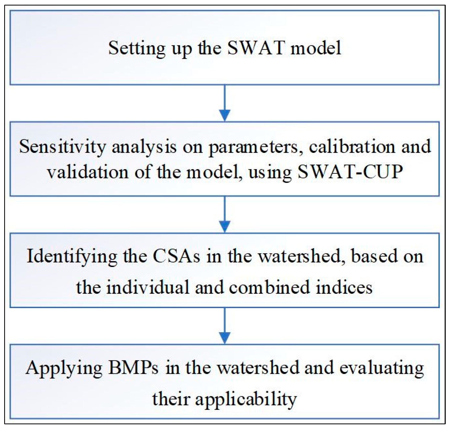
2. Materials and Methods

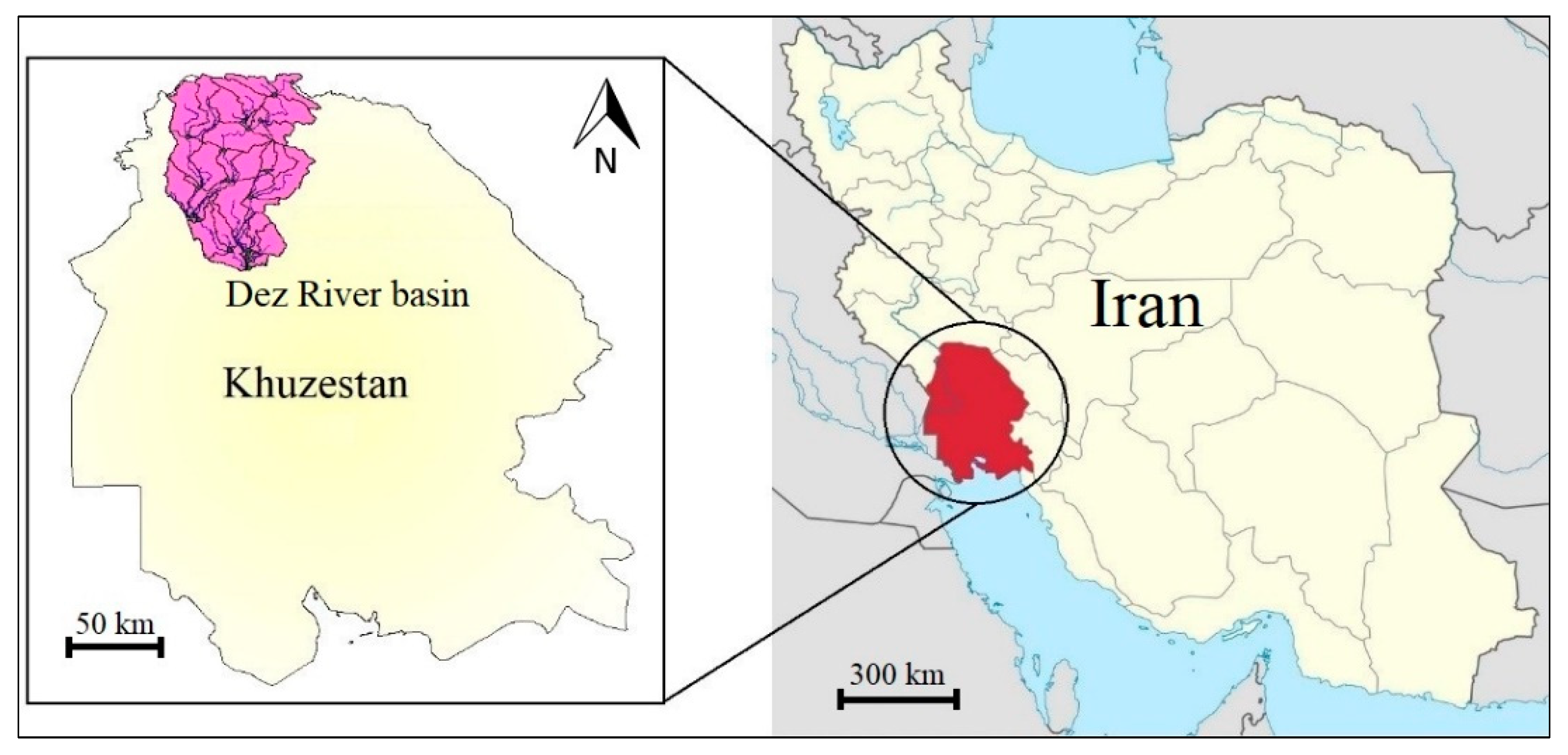
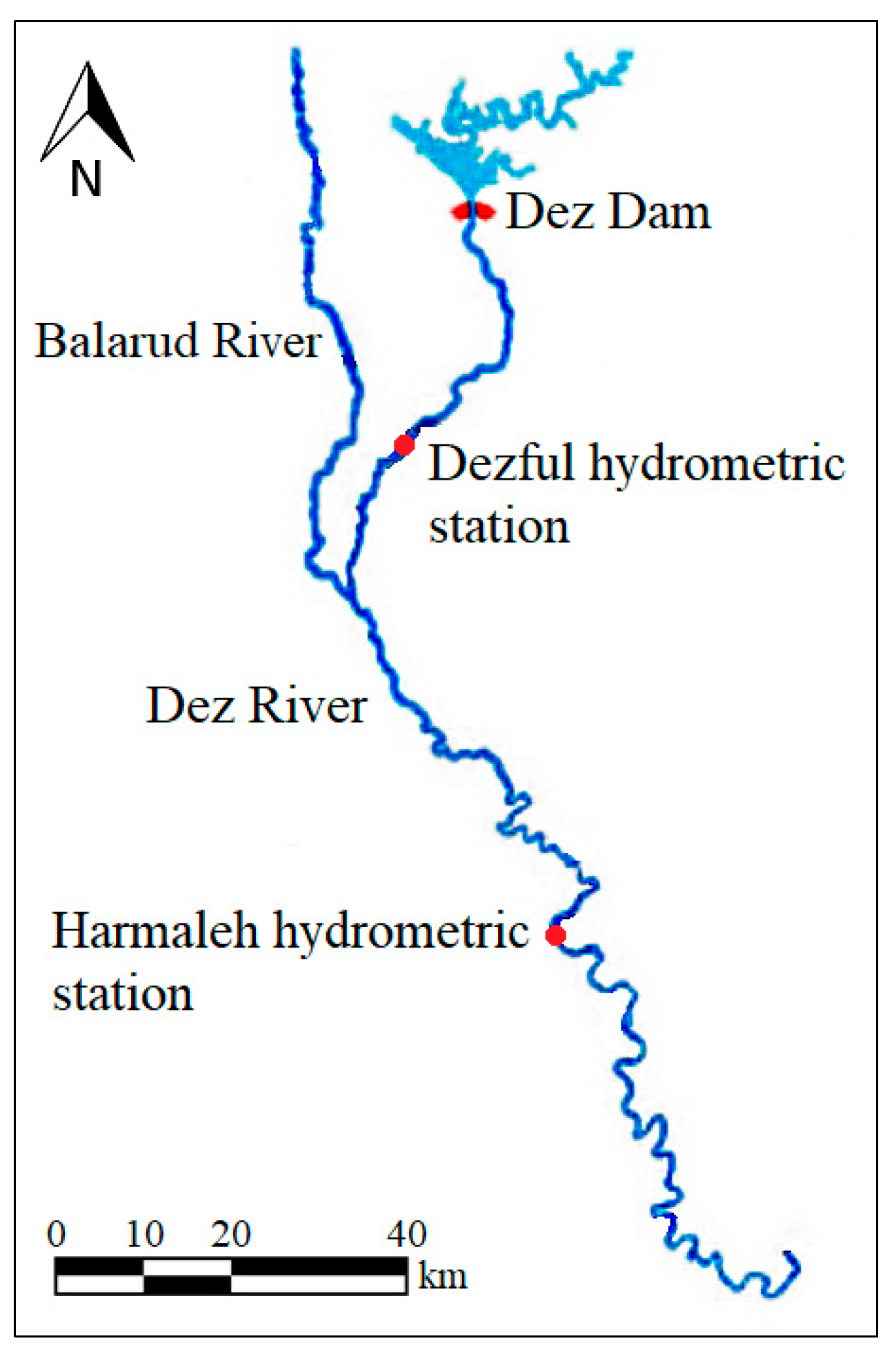
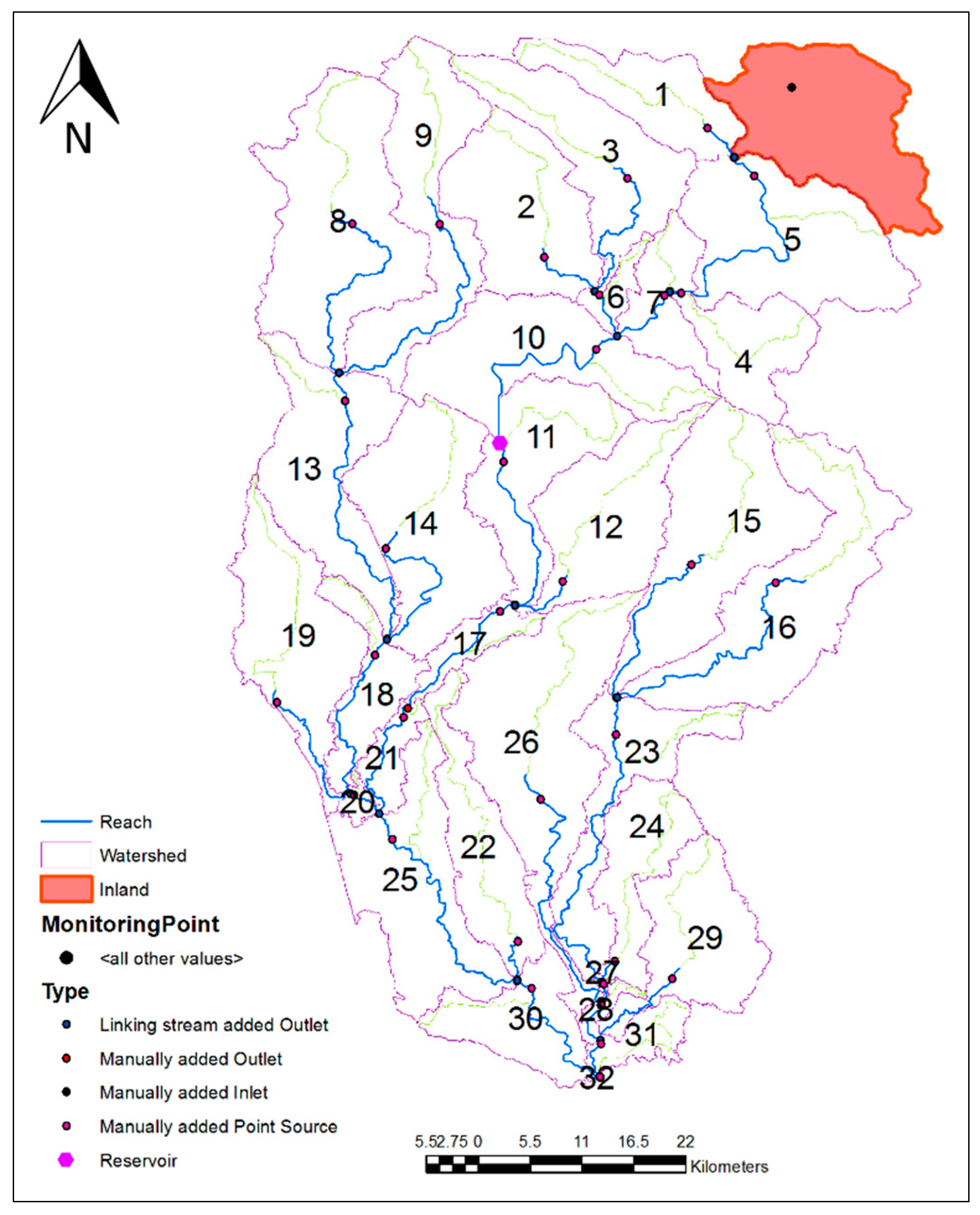
2.1. Study Area and Data

The Dez River basin (556,008 ha) is located in the province of Khuzestan in Iran (Figure 2). Based on the meteorological records (1990–2014), the area receives an average precipitation of 376 mm/year, and the average air temperature in the basin is 25.6 °C. Arable lands constitute 200,000 ha of the region, of which 150,000 ha can be irrigated, and 50,000 ha are cultivated under dryland farming [25]. The major agricultural products in the basin are wheat, sugar cane, and corn, which are cultivated two to three times a year.

Dry and irrigated farming produce 77.34% and 6.3% of the TN load, and 83.56% and 4.3% of the TP load in the basin, respectively. Moreover, residential, pasture, and forest land uses together account for 16.36% of the TN and 12.14% of the TP load in the basin. Three cities of Dezful, Andimeshk, and Shush are located in this basin. Additionally, many villages have been built in the vicinity of the Dez River, and their sewage drains directly into the river. To address these pollution sources, only the city of Dezful has a wastewater treatment plant, which treats 70% of the city’s wastewater. Moreover, three factories in the basin significantly influence the water quality status of the river.

Water quality data scarcity was one of the constraints in this study. In this basin, streamflow data were available at the Dezful and Harmaleh hydrometric stations (Figure 3), while water quality data were only available at the Dezful station.

In order to set up the SWAT model of the Dez River basin, the data presented in

Table 1. The The Soil and Water Assessment Tool (SWAT) model input data.

Data	Source
Digital Elevation Model (DEM)-2011	United States Geological Survey (USGS)
Soil map-2011	FAO Soils Portal
Land use map-2006	Iran’s Forests, Range and Watershed Management Organization
Meteorological data-(1991–2014)	I.R. of Iran Meteorogical Organization
Hydrometric and sediment data-(1991–2014)	Khuzestan Water and Power Authority
Water quality and point source pollution data-2012	Directorate General of Environmental Protection of Khuzestan Province
Management and agricultural data	Royan Consulting Engineers

were used.

2.2. SWAT and SWAT-CUP

The SWAT model is a conceptual, semi-distributive, and continuous river basin scale model [26]. This model requires input data such as topography, soil, and land use maps, as well as meteorological data (precipitation, temperature, wind speed, relative humidity, and solar radiation), inter-basin water transfer data, point source pollution data, and land management practices, in order to simulate the physical processes within a watershed [27]. Based on the soil type, land use, and slope, the SWAT model divides the basin into Hydrological Response Units (HRUs) and runs the simulations at the HRU level [28].

Prior to model calibration, more sensitive parameters have to be identified. Sensitivity analysis is the process of determining the significance of the impact of one parameter, or a combination of parameters, on the output of a model. The SWAT-CUP program has been developed for calibration, validation, and sensitivity analysis of the SWAT model parameters, and uses five different calibration procedures: SUFI-2, Particle Swarm Optimization (PSO), Generalized Likelihood Uncertainty Estimation (GLUE), Parameter Solution (ParaSol), and Markov Chain Monte Carlo (MCMC). For large-scale models, in which the calibration process can be very time-consuming, the semi-automated SUFI-2 is quite efficient. In the SWAT-CUP, the sensitivities of parameters are measured by t-stat values and p-values. Parameters that show higher t-stat values and p-values closer to 0 are more sensitive, and the effect of varying the parameter will be more significant on the target variable [29].

Calibration means adjusting the model input parameters with the goal of achieving the best fit between the observed and simulated values. In the SWAT-CUP, the goodness of calibration is measured using p-factor (the fraction of the data in the range of 95% prediction uncertainty (95ppu)) and r-factor (the average thickness of the 95ppu band, divided by the standard deviation of the observed data). The p-factor is a value between 0 to 1, and the r-factor has a range of 0 to $\infty$. When the p-factor = 1 and the r-factor = 0, the simulated model is precisely in accordance with observed data. p-factors greater than 0.7 and r-factors smaller than 1.5 show satisfactory calibration and validation results.

Another means for evaluation of the goodness of calibration and validation are the coefficient of determination (R²) (Equation (1)) and the Nash-Sutcliffe (NS) model efficiency coefficient (Equation (2)):

$$R^2=\frac{\left[{\sum }_i(Q_{m,i-}{\overline{Q}}_m\right)\left(Q_{s,i}-{\overline{Q}}_s\right){]}^2}{{\sum }_i{\left(Q_{m,i-}{\overline{Q}}_m\right)}^2{\sum }_i{\left(Q_{s,i}-{\overline{Q}}_s\right)}^2}$$

(1)

$$NS=1- \frac{{\sum }_i{\left|Q_m- Q_s\right|}_i^2}{{\sum }_i{\left|Q_{m,i}- {\overline{Q}}_m\right|}_i^2}$$

(2)

where Q is the variable, such as streamflow or sediment; the indices m, and s, represent the observed and simulated values; and Q_avg is the mean of the measured variables.

The NS function has a range of -∞ to 1. NS = 1 corresponds to a perfect match of simulated values to the observed data. The values between 0 and 1 indicate that the simulated and observed values are close to each other, whereas values less than 0 show that the model has no predictive power [30]. The following shows the different work steps in SUFI-2 followed in this study to reduce the parameter uncertainty and to calibrate the model [31]:

• Step 1: The objective function is defined and the absolute range of parameters, based on the recommended values in the software, is set.
• Step 2: Absolute sensitivity analysis is carried out, using Latin Hypercube sampling. The objective function is computed.
• Step 3: The sensitivity matrix of the objective function is calculated. Equivalent of the Hessian matrix is formulated.
• Step 4: High order derivatives are neglected. Based on the Cramer Rao Theorem, an estimate of lower bound of parameter covariance is computed.
• Step 5: Parameter sensitivity is analyzed using multiple regression.
• Step 6: Uncertainty measures (p-factor and r-factor) are computed.

In this study, all of the observed data were used for calibration. Afterward, to validate the calibrated model, while keeping all calibrated parameters constant, the model was run for the last third period of the year (September, October, November, and December).

2.3. Identification of CSAs

The CSAs are areas that produce the highest pollution loads in the basin, and are identified at the sub-basin level [32]. In order to identify the CSAs, sediment and nutrient yields from each sub-basin have to be analyzed based on loads per unit area (tons per hectare per year). Afterward, sub-basins will be ranked in descending order based on yields (the sub-basin with the highest yield will be ranked first). Moving from the highest ranking to the lowest, and based on the analysis of management practices and operational costs, sub-basins that contribute from 5% to 8% (based on the literature) of the sedimentary, TN, or TP loads in the basin will be considered as the CSAs [9].

Combined indices can also be implemented to identify the sub-basins, which can be considered as CSAs. In this method, the CSAs are defined by multi-factors. These factors include a weighted combination of TN, TP, and sediment loads [22]. The combined index can help identify the areas that are critical for multiple stressors, where the implementation of BMPs will be more economical. This index is given by:

$$G_i={\displaystyle \sum ({\omega }_i{G}_{ij})}$$

(3)

$$N{G}_i=\frac{G_i-G_{\min }}{G_{\max }-G_{\min }}$$

(4)

where G_i is the combined index for sub-basin i; G_ij is an index for TN (j = 1); TP (j = 2); and sediment (j = 3). In Equation (4), NG_i is the normalized evaluation variable for the sub-basin i; and G_min and G_max are the lowest and highest ranks for constituent i for the entire basin.

In managerial tasks where the priority of one variable is higher than the others, the variable can be weighted in Equation (3), using the coefficient ω. The weight is subjectively chosen and assigned to each G_i based on its importance, where $\sum {\mathsf{\omega }}_{\mathrm{i}}$ = 1 [9].

2.4. BMPs and Pollution Load Indices

In this study, in order to reduce pollution entry into the Dez River, the following BMPs were implemented: point source pollution elimination (treating the wastewater from residential areas and the effluent of the factories); implementation of 5 m and 10 m filter strips in residential and agricultural lands; a 20% and 50% reduction in livestock grazing in the basin; and management of the main river channel.

Filter strips are vegetated areas that are situated between surface water bodies and cropland, grazing land, forestland, or disturbed land. They are generally used in locations where runoff water leaves a field, with the intention that sediment, organic material, nutrients, and chemicals can be filtered from the runoff water. They are also known as vegetative filter or buffer strips. This practice is primarily used with agricultural fields to control non-point source pollution. In this method, by reducing the velocity of the surface runoff and the deposition of particles, the pollutants, including soil and organic material, are removed. Edge-of-field filter strips are defined in an HRU. Sediment, nutrient, pesticide, and bacteria loads in surface runoff are reduced as the surface runoff passes through the filter strip. In this study, 5 m and 10 m filter strips were used in areas with irrigated farming, and 5 m filter strips were used in residential and dryland farming areas. Equations (5) to (10) represent how the filter strips reduce runoff, sediment load, and nutrient loads in the SWAT model:

R_R = 75.8 − 10.8 ln(R_L) + 25.9 ln(K_SAT)

(5)

S_R(%) = 79.0 − 1.04 S_L + 0.213R_R

(6)

TN_R = 0.036S_R^1.69

(7)

NN_R = 39.4 + 0.584R_R

(8)

TP_R = 0.90S_R

(9)

DP_R = 29.3 + 0.51R_R

(10)

where R_R is the runoff reduction (%); R_L is the runoff loading (mm); K_SAT is the saturated hydraulic conductivity (mm h⁻¹); S_R is the predicted sediment reduction (%); S_L is sediment loading (kg/m²); TN_R is the total nitrogen reduction (%); NN_R is the nitrate nitrogen reduction (%); TP_R is the total phosphorus reduction (%); and DP_R is the dissolved phosphorus reduction (%) [33].

Livestock grazing, which causes damage to plants and production of fertilizer, highly affects the amount of nutrient entry through runoff from rangelands to receiving water bodies. Managing the timing of livestock grazing, reducing the number of livestock, and preventing livestock grazing are among the most popular practices for livestock grazing management. In this study, 20% and 50% reductions in the number of livestock were used as BMPs, and introduced into the model through the Grazing Management Operation in the SWAT model.

Management of the river main channel is done by controlling erosion in the channel wall through mulching, and controlling the amount of vegetation in the channel wall using dense vegetation cover.

Individual and combined indices were used in this study to identify the CSAs. Using individual indices, areas contributing the most to TN, TP, and sediment loads were identified individually. In the next step, by using combined indices, the CSAs for TN + TP, TN + TP + sediment, and TN + TP + 0.1 sediment were identified.

3. Results and Discussion

3.1. Sensitivity Analysis

In order to find the most effective parameters affecting the yields of runoff, sediment, TN, and TP, the sensitivity analysis was performed on each variable separately. In this regard, the sensitivity analysis was performed on runoff parameters. The results of the sensitivity analysis and the calibrated values are presented in

Table 2. Sensitive parameters, and the calibrated values for runoff, sediment, phosphate, and nitrate.

Parameter	Definition	Calibrated Value	t-Stat	p-Value
Parameters Affecting Streamflow
ALPHA_BF.gw	Baseflow alpha factor (1/days)	0.0037	−10.35	0
CH_K2.rte	Effective hydraulic conductivity in main channel alluvium (mm/h)	352.12	4.15	0
OV_N.hru	Manning’s “n” value for overland flow	12.41	2.41	0.016
SOL_AWC.sol	Available water capacity of the soil layer (mm H2O/mm soil)	0.214	1.83	0.067
GW_REVAP.gw	Groundwater “revap” coefficient	0.092	−1.73	0.085
CANMX.hru	Maximum canopy storage (mm H2O)	53.74	−1.63	0.104
CH_S2.rte	Average slope of main channel along the channel length (m/m)	6.7	1.59	0.112
GW_DELAY.gw	Ground water lag time	108.7	−1.48	0.14
Parameters Affecting Sediment Load
SPCON.bsn	The linear parameter for calculating the maximum amount of sediment that can be reentrained during channel sediment routing	0.00116	−41.45	0
SPEXP.bsn	Exponent parameter for calculating sediment reentrained in channel sediment routing	1.015	6.73	0
CH_ERODMO.rte	Erosion rate of the channel	0.457	1.49	0.136
ADJ_PKR.bsn	Peak rate adjustment factor for sediment routing in the sub-basin (tributary channels)	0.907	−0.67	0.5
Parameters Affecting Phosphate Load
ERORGP.hru	Phosphorus enrichment ratio for loading with sediment	2.52	−3.43	0
ORGP_con.hru	Organic phosphorus concentration in runoff, after urban BMP is applied	26.95	2.84	0.004
PSP.bsn	Phosphorus availability index	0.44	0.92	0.42
SOLP_con.hru	Soluble phosphorus concentration in runoff, after urban BMP is applied	0.231	−0.33	0.73
Parameters Affecting Nitrate Load
SOLN_con.hru	Concentration of nitrogen soluble in runoff	0.132	−3.64	0
NPERCO.bsn	Nitrate percolation coefficient	0.172	−2.05	0.172
ERORGN.hru	Organic N enrichment ratio for loading with sediment	2.81	0.119	0.9
K_N.wwq	Michaelis-Menton half-saturation constant for nitrogen (mg N/L)	0.174	0.058	0.953

. In this study, nitrate and phosphate were calibrated/validated as proxies representing TN and TP, respectively.

The results show that the parameters ALPHA_BF (baseflow alpha factor), CH_K2 (effective hydraulic conductivity in main channel alluvium), and OV_N (Manning’s “n” value for overland flow) had the most significant impact on runoff yield.

In addition, other parameters with the highest sensitivity on sediment, phosphate, and nitrate yields were SPCON (linear parameter for calculating the maximum amount of sediment that can be re-entrained during channel sediment routing), ERORGP (phosphorus enrichment ratio for loading with sediment), and SOLN_con (concentration of soluble nitrogen in runoff).

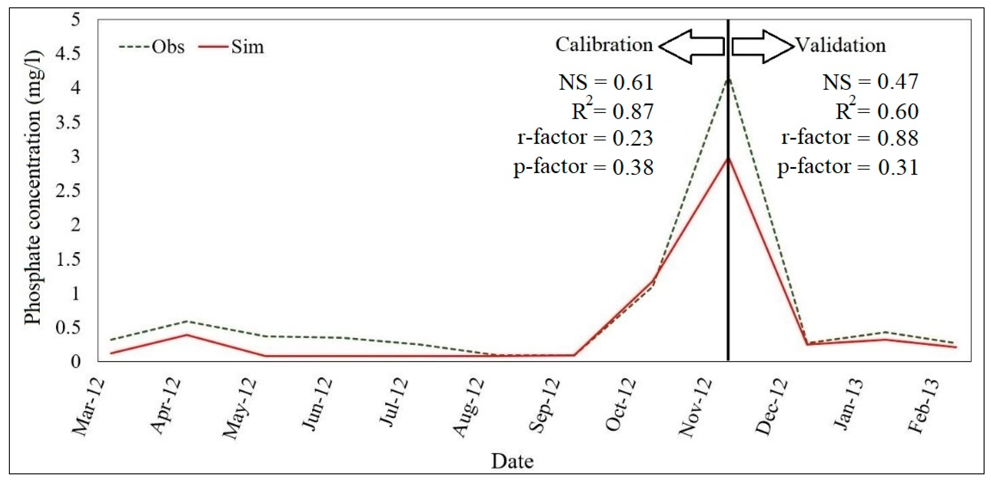
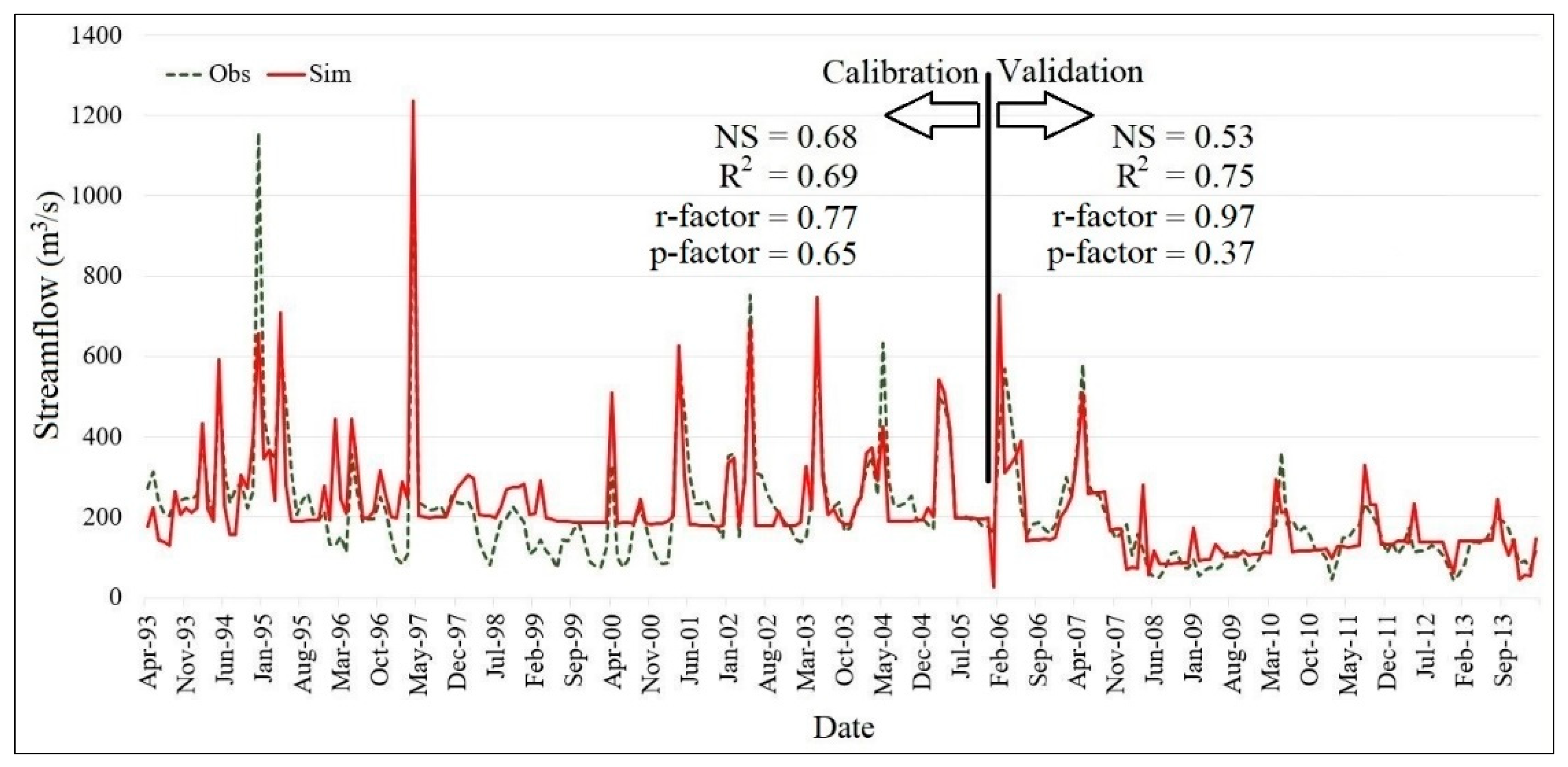
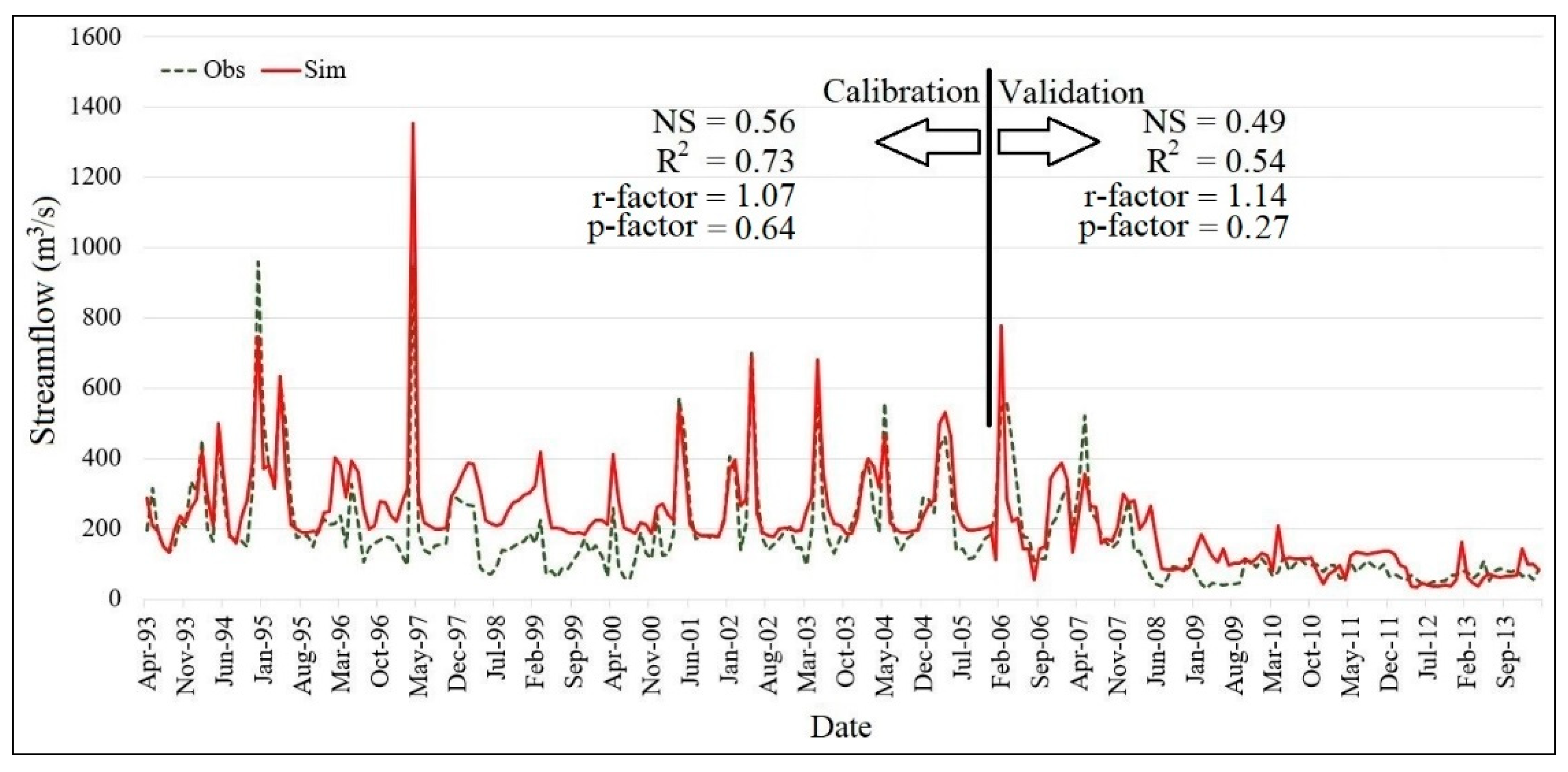
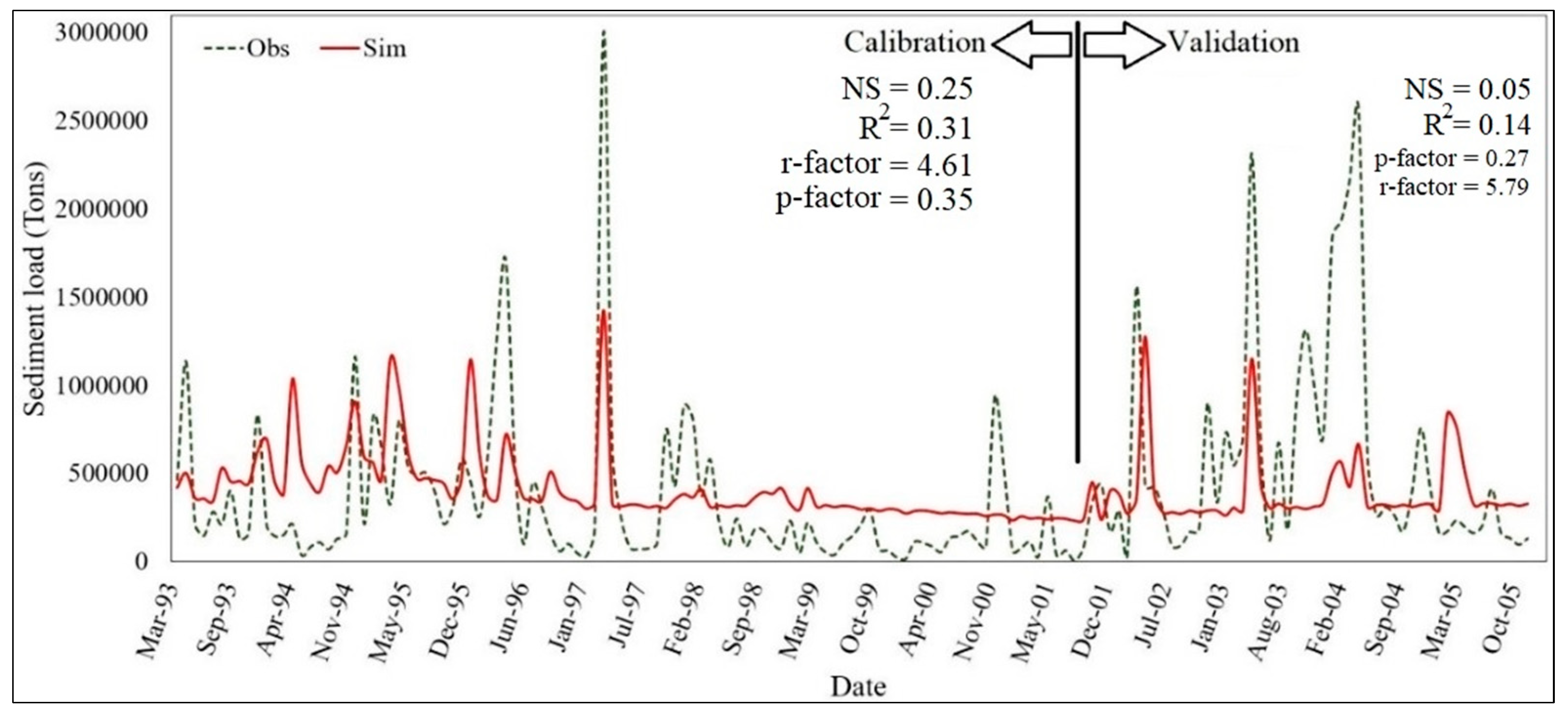
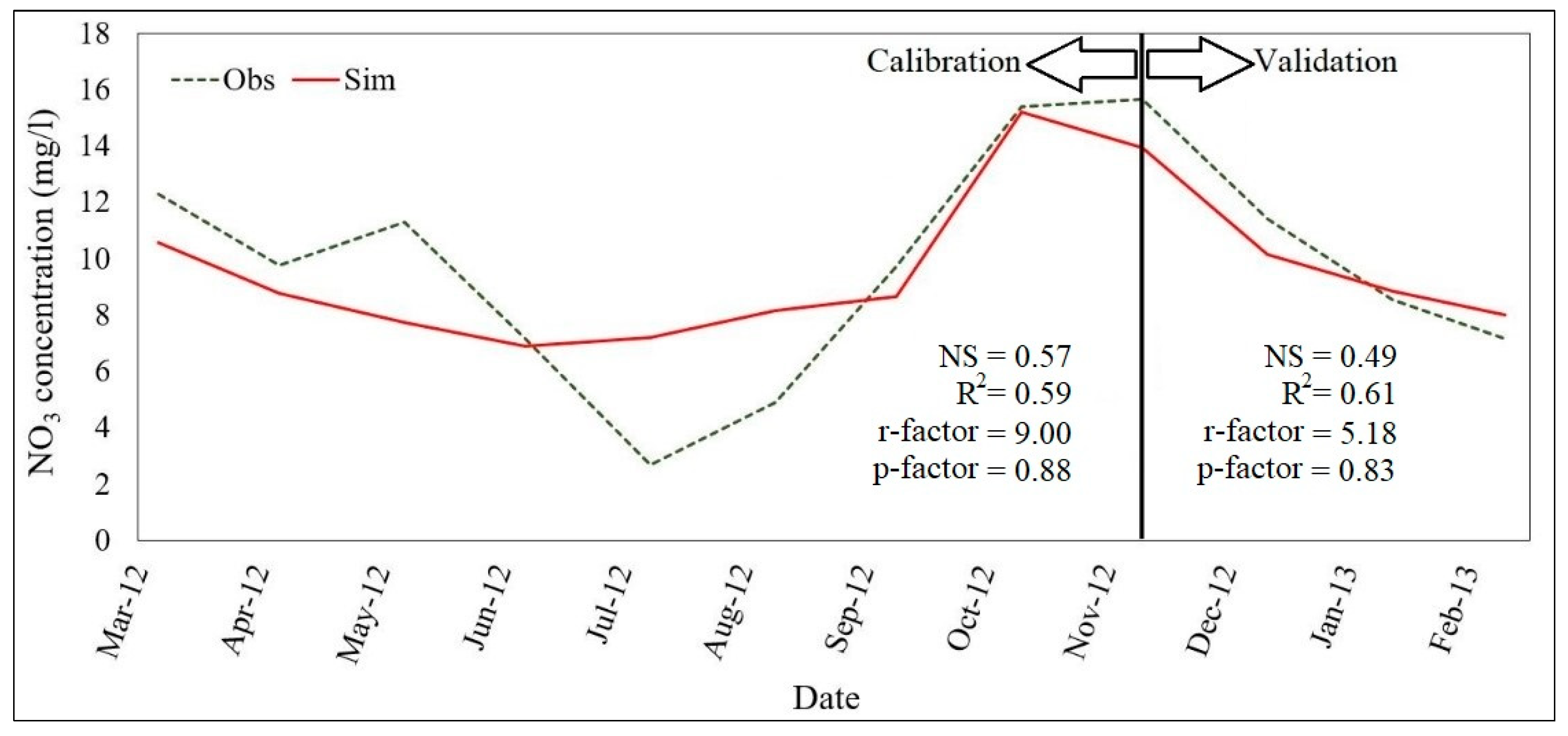
3.2. Calibration and Validation

The calibration and validation of the model were performed in four steps. First, the runoff was calibrated and validated based on the observed data from the Dezful and Harmaleh hydrometric stations. In the next step, nitrate and phosphate were calibrated and validated for the Dezful station. The objective functions of NS, R², p-factor, and r-factor were then used to evaluate the goodness of fit between the simulated and observed values. The results and time series of the simulated data and observational data are presented in Figure 4, Figure 5, Figure 6, Figure 7 and Figure 8.

According to criteria set by Moriasi et al. (2007) [31] for evaluating model performance in calibration and validation, an NS value between 0.50 and 0.65 is considered “satisfactory,” a value between 0.65 and 0.75 is rated as “good,” and “very good” is attributed to values between 0.75 and 1.00. In the calibration process, the sediment calibration was the most difficult. Despite numerous trials on sediment calibration in the model, the peaks could not be simulated. Through field surveys, it was discovered that the locals exploit the river materials, which causes abrupt fluctuations in the sediment load time series. Therefore, high NS values could not be obtained for the sediment during calibration and validation periods. Subsequently, since phosphorus has a tendency to stick to sediment particles, due to uncertainties and limitations in sediment calibration, the simulated phosphate does not show a perfect match with the observed values. However, the NS and R² values are almost in the satisfactory range, both for phosphate and nitrate concentrations.

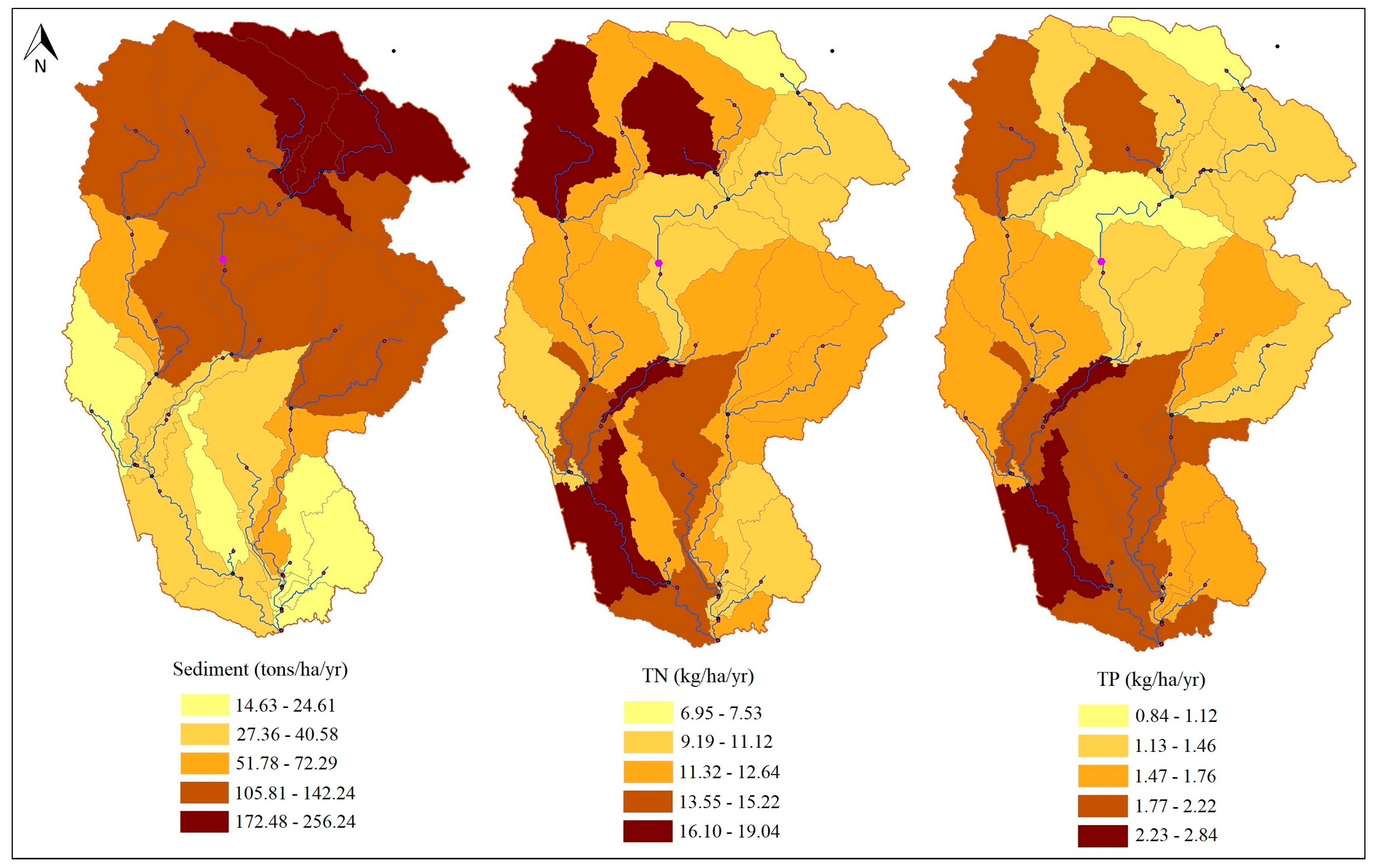
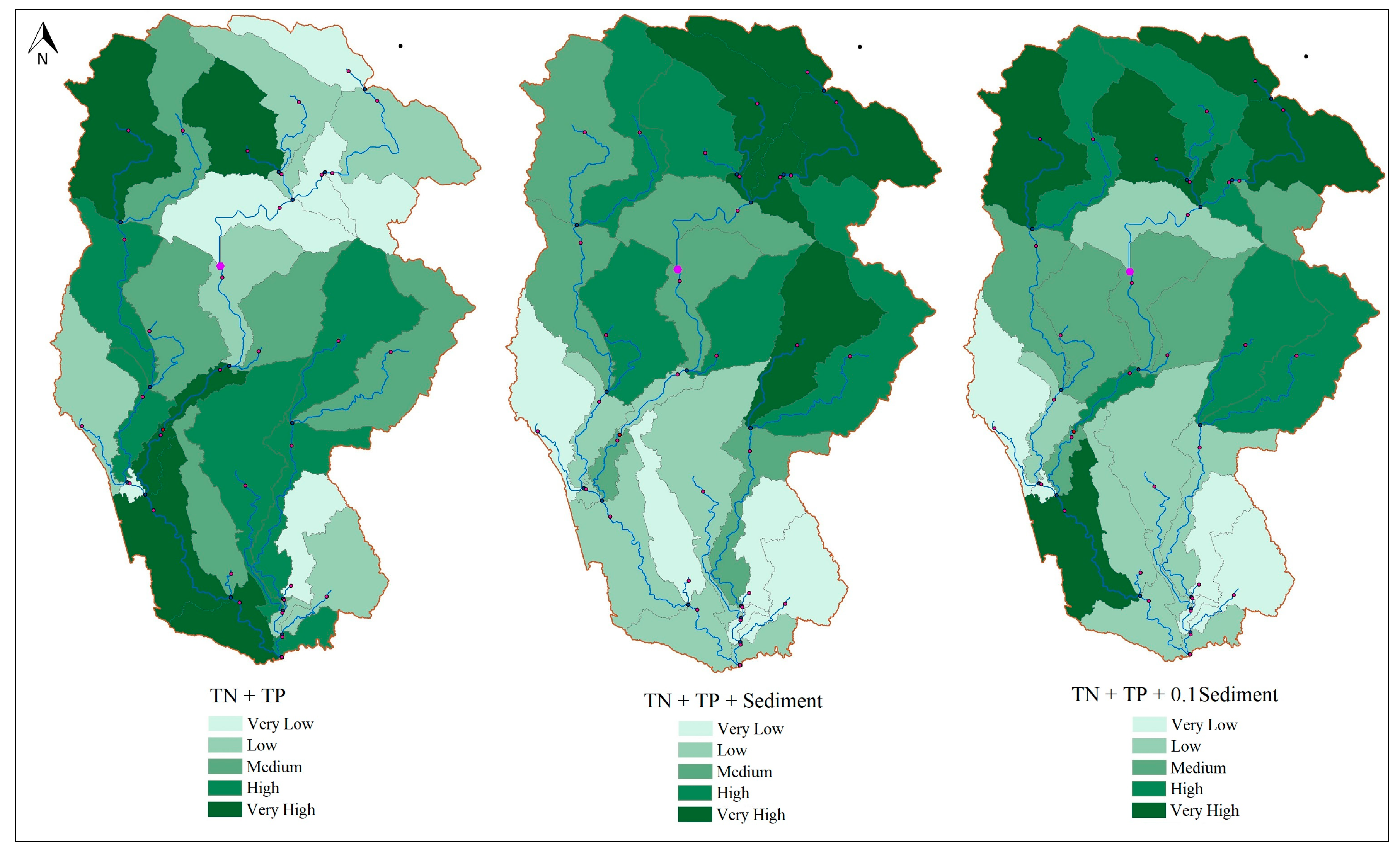
3.3. Identifying the CSAs

Figure 9 shows the delineated Dez River basin in the SWAT model.

Figure 10 shows the results of each analysis using individual indices. Based on the simulation results, the highest erosion rates occurred in the upstream of the basin. Contrary to sediment load, TN and TP loads were higher downstream of the dam, as well as in areas where agricultural activities and population densities are higher, and areas where nomads are located and livestock graze. TN and TP loads upstream of the basin, which is more mountainous and has less agricultural activity than the plains, were much lower than in the downstream area. Sugar cane farms and a factory are located in sub-basin number 25. Therefore, in this sub-basin, the burden of pollution was higher than in the other sub-basins.

Using the combined indices, sub-basins 25 and 17 were identified as the most critical. These sub-basins are located downstream, where the sugar cane factory is located. Subsequently, sub-basins 2 and 8, representing livestock grazing and nomadic settlement sites, were ranked next. By examining the combined indices, it was observed that only introducing nutrient parameters does not provide proper identification of CSAs. By adding sediment to TN and TP, sub-basins 1, 3, 5, and 7 were identified as CSAs due to high sediment loads (because of steep slopes upstream of the river). After applying the 0.1 weight to the sediment, sub-basins 1, 2, 5, 8, and 25 were identified as CSAs. The results of this section are presented in Figure 11.

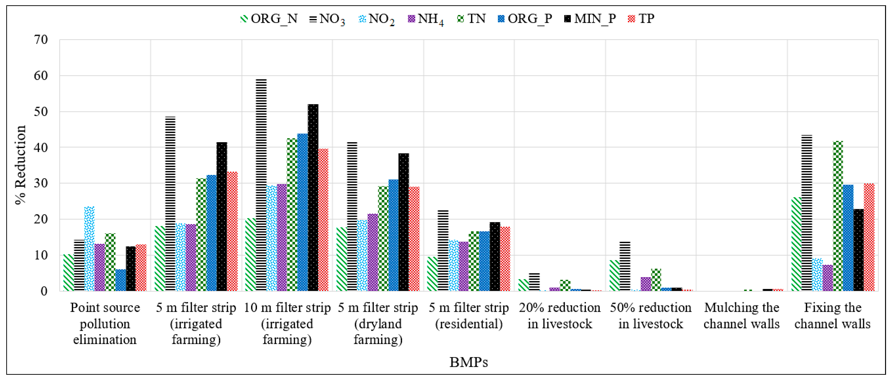
3.4. Evaluation of the BMPs

After identifying the CSAs, the BMPs were implemented in the model to evaluate their applicability in reducing pollution loads. The results of the contaminant reduction, after utilizing BMPs, are presented in

Table 3. Pollution loads reduction after implementation (%) of Best Management Practices (BMPs).

BMP	ORG_N	NO3	NO2	NH4	TN	ORG_P	MIN_P	TP
Point source pollution elimination	10.28	14.4	23.53	13.16	16.21	6.07	12.46	12.98
5 m filter strip (irrigated farming)	18.21	48.51	18.95	18.68	31.48	32.4	41.38	33.28
10 m filter strip (irrigated farming)	20.26	58.92	29.41	29.85	42.61	43.77	51.94	39.57
5 m filter strip (dryland farming)	17.79	41.47	19.71	21.58	29.34	31.09	38.31	29.09
5 m filter strip (residential)	9.62	22.48	14.32	13.81	16.75	16.76	19.18	17.98
20% reduction in livestock	3.37	5.23	0.31	1.02	3.12	0.57	0.54	0.29
50% reduction in livestock	8.71	14.21	0.48	3.94	6.34	0.97	0.96	0.43
Mulching the channel walls	0.1	0.08	0.03	0.07	0.43	0.19	0.58	0.62
Fixing the channel walls	26.1	43.4	9.12	7.37	41.78	29.56	22.96	30.01

and Figure 12.

Removing point source pollution by constructing a treatment plant reduced the nitrite (23.53%) and ammonia (13.16%) from the domestic and industrial sewage in the river. The highest reduction in pollution load was achieved by implementing filter strips in the agricultural areas. Under this BMP, the highest reduction in pollutants was observed for nitrate (58.92%). Furthermore, the results indicated that by increasing the length of the filter strips, the TN load was reduced more than the TP. Reductions of 20% and 50% in the number of livestock were more effective in reducing the amount of nitrate (5.23% and 14.21%) and organic nitrogen (3.37% and 8.71%), compared to the other nutrients. However, this BMP did not show a significant impact on the amount of phosphorous compounds.

River channel wall mulching had little impact on reducing the nutrients, and only decreased the amount of sediment input into the river. Due to the tendency of phosphorus to stick to sediment particles, the only observed effect of this strategy was in reducing the phosphorous compounds in the river.

4. Conclusions

In this study, the Dez River basin in Iran was modeled using the SWAT model, and the sensitivity analysis and calibration/validation of the model were performed using the SUFI-2 algorithm of the SWAT-CUP software. After delineation of the basin, the CSAs were identified based on the amount of pollution produced in each sub-basin, using individual and combined indices. Moreover, several BMPs, including source elimination, filter strips (5 m and 10 m), livestock grazing management, and river channel management were implemented to evaluate their applicability in reducing the entry of pollutants to the river. The following are the main findings of this study:

• A significant decrease in TN (42.61%) and TP (39.57%) loads were observed in areas with irrigated farming where 10 m filter strips were implemented.
• Reducing the number of livestock was not effective in reducing phosphorous compounds.
• The mulching of the river channel walls did not have much impact on reducing pollution.
• Using combined indices to identify CSAs without weighting variables is not desirable, and CSAs should be weighed according to the priority of the variables.

For future studies, considering climate change and its consequences, the researchers recommend evaluating the management practices by changing inputs such as precipitation, relative humidity, and solar radiation, and then reassessing the adequacy of these practices in future studies.

References

1. Dawadi, S.; Ahmad, S. Evaluating the Impact of Demand-Side Management on Water Resources under Changing Climatic Conditions and Increasing Population. J. Environ. Manag. 2013, 114, 261–275. [Google Scholar] [CrossRef]
2. Ahmad, S. Managing Water Demands for a Rapidly Growing City in Semi-Arid Environment: Study of Las Vegas, Nevada. Int. J. Water Res. Arid Environ. 2016, 5, 35–42. [Google Scholar]
3. Amoueyan, E.; Ahmad, S.; Eisenberg, J.; Pecson, B.; Gerrity, D. Quantifying Pathogen Risks Associated with Potable Reuse: A Risk Assessment Case Study for Cryptosporidium. Water Res. 2017, 119, 252–266. [Google Scholar] [CrossRef]
4. Choubin, B.; Khalighi-Sigaroodi, S.; Malekian, A.; Ahmad, S.; Attarod, P. Drought Forecasting in a Semi-Arid Watershed Using Climate Signals: A Neuro-Fuzzy Modeling Approach. J. Mount. Sci. 2014, 11, 1593–1605. [Google Scholar] [CrossRef]
5. Huang, J.; Lin, J.X.; Wang, J. The Precipitation Driven Correlation Based Mapping Method (PCM) for Identifying the Critical Source Areas of Non-Point Source Pollution. J. Hydrol. 2005, 524, 100–110. [Google Scholar] [CrossRef]
6. Thakali, R.; Kalra, A.; Ahmad, S.; Qaiser, K. Management of An Urban Stormwater System Using Projected Future Scenarios of Climate Models: A Watershed-Based Modeling Approach. Open Water J. 2018, 5, 1. [Google Scholar]
7. Venkatesan, A.; Ahmad, S.; Johnson, W.; Batista, J. System Dynamics Model to Forecast Salinity Load to the Colorado River Due to Urbanization within the Las Vegas Valley. Sci. Total Environ. 2011, 409, 2616–2625. [Google Scholar] [CrossRef]
8. Natha, S.B.; Allan, J.D.; Dolan, D.M.; Han, H.; Richards, R.P. Application of the Soil and Water Assessment Tool for Six watersheds of Lake Erie: Model parameterization and calibration. J. Great Lakes Res. 2011, 37, 263–271. [Google Scholar] [CrossRef]
9. Niraulaa, R.; Kalinb, L.; Srivastavac, P.; Anderson, C.J. Identifying Critical Source Areas of Non-Point Source Pollution with SWAT and GWLF. Ecol. Model. 2013, 268, 123–133. [Google Scholar] [CrossRef]
10. Panagopoulos, Y.; Makropoulos, C.; Mimikou, M. Decision Support for Diffuse Pollution Management. Environ. Model. Softw. 2012, 30, 57–70. [Google Scholar] [CrossRef]
11. Nazari-Sharabian, M.; Ahmad, S.; Karakouzian, M. Climate Change and Eutrophication: A Short Review. Eng. Technol. Appl. Sci. Res. 2018, 8, 3668–3672. [Google Scholar] [CrossRef]
12. Chaplot, V.; Saleh, A.; Jaynes, D.B.; Arnold, J.G. Predicting Water, Sediment, and NO3-N Loads Under Scenarios of Land-Use and Management Practices in a Flat Watershed. Water Air Soil Pollut. 2014, 154, 271–293. [Google Scholar] [CrossRef]
13. Santhi, C.; Srinivasan, R.; Arnold, J.G.; Williams, J.R. A Modeling Approach to Evaluate the Impacts of Water Quality Management Plans Implemented in a Watershed in Texas. Environ. Model. Softw. 2006, 21, 1141–1157. [Google Scholar] [CrossRef]
14. Ghumman, A.R.; Ahmad, S.; Khan, R.A.; Hashmi, H.N. Comparative Evaluation of Implementing Participatory Irrigation Management in Punjab Pakistan. Irrig. Drain. 2014, 63, 315–327. [Google Scholar] [CrossRef]
15. Pisinaras, V.; Petalas, C.; Gikas, G.D.; Gemitzi, A.; Tsihrintzis, V.A. Hydrological and Water Quality Modeling in a Medium-Sized Basin Using the Soil and Water Assessment Tool (SWAT). Desal 2009, 250, 274–286. [Google Scholar] [CrossRef]
16. Bracmort, K.S.; Arabi, M.; Frankenberger, J.R.; Engel, B.A.; Arnold, J.G. Modeling Long-Term Water Quality Impact of Structural BMPs. Trans. ASABE 2006, 49, 367–374. [Google Scholar] [CrossRef]
17. Santhi, C.; Arnold, J.G.; Williams, J.R.; Hauck, L.M.; Dugas, W.A. Application of a Watershed Model to Evaluate Management Effects on Point and Nonpoint Source Pollution. Trans. ASABE 2001, 44, 1559–1570. [Google Scholar] [CrossRef]
18. Bouraoui, F.; Benabdallah, S.; Jrad, A.; Bidoglio, G. Application of the SWAT Model on the Medjerda River Basin (Tunisia). Phys. Chem. Earth 2005, 30, 497–507. [Google Scholar] [CrossRef]
19. Arabi, M.; Govindaraju, R.S.; Hantush, M.M. Cost-Effective Allocation of Watershed Management Practices Using a Genetic Algorithm. Water Resour. Res. 2006, 42, W10429. [Google Scholar] [CrossRef]
20. Ficklin, D.L.; Luo, Y.; Zhang, M. Watershed Modelling of Hydrology and Water Quality in the Sacramento River Watershed, California. Hydrol. Process. 2012, 27, 236–250. [Google Scholar] [CrossRef]
21. Zhang, X.; Zhang, M. Modeling Effectiveness of Agricultural BMPs to Reduce Sediment Load and Organophosphate Pesticides in Surface Runoff. Sci. Total Environ. 2012, 409, 1949–1958. [Google Scholar] [CrossRef]
22. Liu, R.; Xu, F.; Zhang, P.; Yu, W.; Men, C. Identifying Non-Point Source Critical Source Areas Based on Multi-Factors at a Basin Scale with SWAT. J. Hydrol. 2016, 533, 379–388. [Google Scholar] [CrossRef]
23. Dong, F.; Liu, Y.; Wu, Z.; Chen, Y.; Guo, H. Identification of Watershed Priority Management Areas under Water Quality Constraints: A Simulation-Optimization Approach with Ideal Load Reduction. J. Hydrol. 2018, 562, 577–588. [Google Scholar] [CrossRef]
24. Qiu, J.; Shen, Z.; Huang, M.; Zhang, X. Exploring Effective Best Management Practices in the Miyun Reservoir Watershed. China Ecol. Eng. 2018, 123, 30–42. [Google Scholar] [CrossRef]
25. Agricultural Comprehensive Plan of Khuzestan Province. Available online: http://ajkhz.ir/main/ (accessed on 15 January 2019).
26. Arnold, J.G.; Srinivasan, R.; Muttiah, R.S.; Allen, P.M. Large Area Hydrologic Modeling and Assessment Part I: Model development. J. Am. Water Resour. 1999, 34, 37–89. [Google Scholar] [CrossRef]
27. Kiniry, J.R.; Williams, J.R.; King, K.W. Soil and Water Assessment Tool Theoretical Documentation, version 2009; Center for Agricultural & Rural Development: Ames, IA, USA, 2011; p. 618. [Google Scholar]
28. Shang, X.; Wang, X.; Zhang, D.; Chen, W.; Chen, X.; Kong, H. An Improved SWAT-Based Computational Framework for Identifying Critical Source Areas for Agricultural Pollution at the Lake Basin Scale. Ecol. Model. 2012, 226, 1–10. [Google Scholar] [CrossRef]
29. Abbaspour, K.C.; Yang, J.; Maximov, I.; Siber, R.; Bogner, K.; Mieleitner, J.; Zobrist, J.; Srinivasan, R. Modelling Hydrology and Water Quality in the Pre-Alpine/Alpine Thur Watershed using SWAT. J. Hydrol. 2007, 333, 413–430. [Google Scholar] [CrossRef]
30. Nash, J.E.; Sutcliffe, J.V. River Flow Forecasting Through Conceptual Models: Part 1—A Discussion of Principles. J. Hydrol. 1970, 10, 282–290. [Google Scholar] [CrossRef]
31. Moriasi, D.N.; Arnold, J.G.; Van Liew, M.W.; Bingner, R.L.; Harmel, R.D.; Veith, T.L. Model Evaluation Guidelines for Systematic Quantification of Accuracy in Watershed Simulations. Trans. ASABE 2007, 50, 885–900. [Google Scholar] [CrossRef]
32. Winchell, M.F.; Folle, S.; Meals, D. Using SWAT for Sub-Field Identification of Phosphorus Critical Source Areas in a Saturation Excess Runoff Region. Hydrol. Sci. J. 2015, 60, 844–862. [Google Scholar] [CrossRef]
33. White, M.J.; Arnold, J.G. Development of a Simplistic Vegetative Filter Strip Model for Sediment and Nutrient Retention at the Field Scale. Hydrol. Proc. 2009, 23, 1602–1616. [Google Scholar] [CrossRef]
Figure 1. The flowchart of this study.
Environments 06 00020 g001
Figure 2. The geographic location of the Dez River basin.
Environments 06 00020 g002
Figure 3. Hydrometric stations.
Environments 06 00020 g003
Figure 4. Calibration (1993–2005) and validation (2006–2014) of monthly streamflow in Dezful station.
Environments 06 00020 g004
Figure 5. Calibration (1993–2005) and validation (2006–2014) of monthly streamflow in Harmaleh station.
Environments 06 00020 g005
Figure 6. Calibration and validation of monthly sediment load in Dezful station (2012–2013).
Environments 06 00020 g006
Figure 7. Calibration and validation of monthly phosphate concentration in Dezful station (2012–2013).
Environments 06 00020 g007
Figure 8. Calibration and validation of monthly nitrate concentration in Dezful station (2012–2013).
Environments 06 00020 g008
Figure 9. The delineated Dez River basin in the SWAT model.
Environments 06 00020 g009
Figure 10. The Critical Source Areas (CSAs) in the basin, identified using individual indices.
Environments 06 00020 g010
Figure 11. The CSAs in the basin, identified using combined indices.
Environments 06 00020 g011
Figure 12. Reduction in pollution loads after utilizing the BMPs.
Environments 06 00020 g012