
Variability of Remotely Sensed Solar-Induced Chlorophyll Fluorescence in Relation to Climate Indices


1
Wharton School, University of Pennsylvania, Philadelphia, PA 19104, USA
2
Nicholas School of the Environment, Duke University, Durham, NC 27708, USA
3
Department of Marine, Earth and Atmospheric Sciences, North Carolina State University, Raleigh, NC 27695, USA
*
Author to whom correspondence should be addressed.
Environments 2022, 9(9), 121; https://doi.org/10.3390/environments9090121
Submission received: 12 December 2021
/
Revised: 6 September 2022
/
Accepted: 13 September 2022
/
Published: 19 September 2022
(This article belongs to the Special Issue Impacts of Climate Change on the Water–Energy–Food Nexus)
Abstract
:Global remote sensing of solar-induced fluorescence (SIF), a proxy for plant photosynthetic activity, represents a breakthrough in the systematic observation of global-scale gross primary production and other ecosystem functions. Here, we hypothesize that all earth ecosystem variabilities, including SIF, are affected by climate variations. The main contribution of this study is to apply a global empirical orthogonal function (EOF) analysis of SIF to quantify the relations between the large-scale GPP variability and climate variations. We used 2007–2019 SIF data derived from the Global Ozone Monitoring Experiment-2 (GOME-2) satellite sensor observations and a rotated empirical orthogonal function (EOF) analysis to explore global SIF variability over years and decades. The first leading EOF mode captures the well-known ENSO pattern, with most of the variance over continents in the tropical Pacific and Indian Oceans. The second and third leading EOF modes in SIF variability are significantly related to the NAO and PDO climate indices, respectively. Our analysis also shows that the 2011 La Niña (2015 El Niño) elevated (decreased) global SIF.
1. Introduction
Solar-induced fluorescence (SIF) is a proxy of plant photosynthetic activity. When plants absorb a certain spectrum band of sunlight, some of the energy is emitted as fluorescence, which is detected as SIF. The first record of SIF was made almost two centuries ago by Sir David Brewster, who discovered that a beam of sunlight striking a green alcoholic extract of laurel leaves elicited a brilliant red light [1,2]. SIF can be retrieved from reflected radiance measured by satellite-borne instruments. Research has shown that SIF is correlated with gross primary productivity (GPP; e.g., [3,4,5,6,7,8,9,10]). In particular, changes in SIF magnitude at wavelengths greater than 740 nm are shown to be sufficient for tracking photosynthetic dynamics [11]. Therefore, SIF is a useful variable for certain environmental applications, including indicating changes in vegetation in response to climate change and natural disasters.
Significant advancements have been made in the last decades in the remote sensing observations of SIF and GPP. Such efforts were first made with the Greenhouse Gases Observing Satellite (GOSAT, [12,13]), then with the Global Ozone Monitoring Experiment-2 (GOME-2), the Scanning Imaging Absorption Spectrometer for Atmospheric Chartography (SCIAMACHY, [14]), and the Orbiting Carbon Observatory (OCO-2; [5]). Among these, GOME-2 is a European instrument deployed on the MetOp-A satellite. It was launched on October 19, 2006 to continue the long-term monitoring of atmospheric ozone started by GOME-2 on ERS-2 and SCIAMACHY on Envisat. Because different gases in the atmosphere absorb different wavelengths of light, the GOME-2 scanning spectrometer is designed to capture light reflected from the Earth’s surface and atmosphere and use it to map concentrations of atmospheric ozone, nitrogen dioxide, sulfur dioxide, SIF, and other ultraviolet radiation. It has daily global coverage. Its nadir field of view on the ground is 80 km × 40 km. As such, GOME-2 can make a significant contribution to climate research while providing near real-time data for use in SIF, GPP, and air quality research.
The decade-long satellite-derived SIF has provided a good opportunity to explore interannual to decadal variations in SIF and GPP. Here, we hypothesize that all earth ecosystem variability, including GPP and its proxy SIF, are affected by climate variations. The main contribution of this study is to apply a global empirical orthogonal function (EOF) analysis of SIF to systematically quantify the relations between the large-scale GPP variability and climate variations.
The EOF technique was chosen because it can separate the spatiotemporal signal into a sum of orthogonal modes by maximizing the variance explained by each mode. It has been widely used in oceanography and atmospheric research (e.g., [15,16,17]). We recognize that several very recent studies (e.g., [18,19,20,21,22,23]) have successfully applied machine learning methods to generate additional higher spatial resolutions (e.g., 0.05°) and finer temporal resolution (e.g., 4-day) SIF reconstructions using GOME-2 and SCIAMACHY datasets. For our research purpose, we decided to use the original, GOME-2 0.5 degree, monthly SIF data because: (1) we tried to avoid possible complications associated with inter-sensor calibrations across different satellite sensor platforms [24]; and (2) our focus was on the large-scale signals connected with climate trends and variability rather than high-frequency, small-scale signals that are often driven by local-processes.
This manuscript is organized as follows. Section 2 describes the datasets, climate indices, and the analytical method. Section 3 presents the global EOF analysis and relates the results to regional climate indices. We also compare and contrast SIF conditions in 2011 and 2015 to explore the impact of ENSO on the global SIF variability. Concluding remarks are given in Section 4.
2. Data and Methods
2.1. SIF Data
We used the GOME-F version 28 (V28) terrestrial chlorophyll fluorescence data retrieval, produced by Dr. Joanna Joiner ([24,25,26]) as part of a NASA Making Earth System Data Records for Use in Research Environments program. V28 retrievals use GOME instrument channel 4 with ~0.5 nm spectral resolution and wavelengths between 734 and 758 nm. The Level 3 data are available (https://avdc.gsfc.nasa.gov/pub/data/satellite/MetOp/GOME_F/v28/MetOp-A/level3/, accessed on 15 June 2021) at 0.5° spatial resolution and at monthly temporal resolution and cover February 2007 to March 2019.
GOME-F products are inherently noisy due to low signal levels. We used the estimated monthly SIF values contained in the products. Because the GOME instrument has a relatively large observation footprint, clouds and aerosols are present in nearly every daily observation. Various filtering techniques were applied ([26]), but cloud-contaminated data are still present in a significant portion of the monthly mean data. To address the noisy data and cloud cover problems, we applied a seven-point median box filter in space and a three-month running mean filter in time to generate a gap-free monthly time series of SIF (Figure 1). Such smoothing degrades the time and space resolution of features. For example, small-scale vegetation changes over steep terrains cannot be resolved in the smoothed imagery, nor can the effects of events having time scales of days to weeks be fully resolved. Nevertheless, the data processing approach adopted herein is justified because the focus of this study is the global, continental-scale features that occur on interannual to decadal timescales.
2.2. Climate Indices
We considered several key climate modes in this study. The most significant mode is arguably the El Niño–Southern Oscillation (ENSO, [27]). Other important modes include the Atlantic multidecadal oscillation (AMO, [28]), the North Atlantic Oscillation (NAO, [29]), and the Pacific decadal oscillation (PDO, [30]). Numerical indices that define these modes of climate variability are briefly introduced below.
2.2.1. El Niño–Southern Oscillation (ENSO)
ENSO shifts irregularly back and forth between El Niño and La Niña every few years. Each phase triggers disruptions of temperature, precipitation, winds, and ocean circulation and thus has profound global impacts. El Niño conditions occur when abnormally warm waters accumulate in tropical latitudes of the central and eastern Pacific Ocean. Consequently, tropical rains that usually fall over the western Pacific shift eastward. During El Niño, regions in the western Pacific typically face severe drought conditions, while northwestern North America is more likely to experience warmer-than-average temperatures and more rain. La Niña conditions occur when cooler-than-average waters accumulate in the central and eastern tropical Pacific and tropical rains shift to the west. Seasonal precipitation impacts are generally opposite those of El Niño. The Niño 3.4 Index is an indicator used by NOAA for monitoring the ENSO state. It tracks the running three-month average of sea surface temperature (SST) in the east-central tropical Pacific between 120° and 170° W, called the Niño 3.4 region. This running three-month average SST is compared to a previous 30 year (1981–2010) mean SST to calculate SST anomaly. The El Niño condition is considered to be present when the temperature anomaly is +0.5 °C or higher, indicating the east-central tropical Pacific is significantly warmer than usual. La Niña conditions exist when the index is −0.5 °C or lower, indicating the region is cooler than usual. The Niño 3.4 Index is essentially a time series of SST anomaly. Its monthly time series is processed by NOAA and available at: https://psl.noaa.gov/gcos_wgsp/Timeseries/Nino34/ (accessed on 15 June 2021).
2.2.2. Atlantic Multidecadal Oscillation (AMO)
The AMO represents long-duration changes in the sea surface temperature of the North Atlantic Ocean, with cool and warm phases alternating; each may last for 20–40 years. It is quantified by the average SST anomalies in the North Atlantic basin between 0–70° N. Since 1994, the AMO has been in a warm phase. The AMO has affected air temperatures and rainfall over much of the northern hemisphere, especially North America and Europe. It is associated with changes in the frequency of North American droughts. During AMO warm phases, most of North America receives less than normal rainfall. The detrended monthly AMO time series is available at: https://psl.noaa.gov/gcos_wgsp/Timeseries/AMO/ (accessed on 15 June 2021).
2.2.3. North Atlantic Oscillation (NAO)
The NAO is defined as the normalized pressure difference between the Icelandic Low and the Azores High ([29]). Through fluctuations in their strength, the NAO controls the speed and direction of westerly winds and location of storm tracks across the North Atlantic. In years when the NAO is positive, westerlies are strong, summers are cool, winters are mild, and rain is frequent. When NOA is negative, westerlies are suppressed, the temperature is more extreme in summer and winter leading to heat waves, deep freezes, and reduced rainfall. The normalized, monthly NAO time series is available at: https://psl.noaa.gov/gcos_wgsp/Timeseries/NAO/ (accessed on 15 June 2021).
2.2.4. Pacific Decadal Oscillation (PDO)
The PDO is a recurring pattern of ocean–atmosphere climate variability centered over the Pacific basin north of 20° N. During the positive phase, the west Pacific becomes cooler and part of the eastern Pacific warms. The wintertime Aleutian Low is deepened and shifted southward, advecting warm, humid air along the North American west coast. Air temperatures are higher than usual from the northwest North America to Alaska but below normal in Mexico and the southeastern United States. Winter precipitation is higher than usual in the Alaska Coast Range, Mexico, and the southwestern United States but reduced over Canada, eastern Siberia, and Australia ([30]). During a negative phase, the opposite pattern occurs.
The PDO index is derived by performing an EOF analysis on monthly sea surface temperature anomalies over the North Pacific after the global average sea surface temperature has been removed. The PDO index is the leading principal component time series. Its monthly time series is available at: https://psl.noaa.gov/gcos_wgsp/Timeseries/PDO/ (accessed on 15 June 2021).
2.3. Rotated EOF
The 13-year, gridded, cloud-free SIF data allow us to investigate the temporal and spatial variability of SIF/GPP at the global scale by decomposing these multidimensional fields into empirical orthogonal functions (EOFs, [31,32,33,34,35,36,37]). We focused on 65° S to 65° N to concentrate the analysis of SIF/GPP variations in the non-polar regions. By organizing the SIF data in an M × N matrix, where M and N represent the spatial (187,200 grid points) and temporal (146 months) elements, respectively, we can represent the SIF data matrix, s(x, t) by
where x represents the spatial coordinates (longitude, latitude), and t represents the time coordinate. ak is the temporal evolution functions (or the principal components), and Fk is the spatial eigenfunctions (or the EOF) for each mode, respectively.
Prior to the EOF analysis, temporal mean and trend were removed from the SIF fields. Because SIF data contain strong seasonal cycles (Figure 1) that are not a focus of this study, we also removed the seasonal cycle by subtracting the long-term monthly mean SIF fields from each corresponding month in the 17-year time series. The resulting detrended, demeaned, and deseasoned data matrix constitutes the input for the EOF analysis. Solving EOF problem then entails the application of singular value decomposition (SVD) to break the covariance of SIF data into three matrices
where U and V are orthonormal and D is diagonal. Then EOFs , and the principal component .
Because of its orthogonality constraint, EOF analysis is known to have a tendency to produce unphysical modes, especially for data covering a large domain. Previous studies have shown that the drawbacks of EOF analysis can be alleviated by rotated EOF (REOF) analysis to better pick up localized patterns (e.g., [38]). We took this approach by performing an orthogonal EOF rotation known as varimax rotation ([39]). This procedure reduces the variances in the projection of the data, thereby putting the EOF basis closer to the actual data variability and increasing physical interpretability.
3. Results and Discussion
3.1. SIF Mean Analysis
The magnitude and spatial pattern of the global monthly mean SIF averaged over 2007 to 2019 (Figure 1) show the highest SIF values in the tropical regions, intermediate values in the eastern United States, southeast Asia, and central Europe, and the lowest values in the barren regions (e.g., deserts, poles). This pattern is largely dependent on local climate conditions (air temperature, precipitation, and solar radiation) as well as vegetation types (e.g., [40,41,42,43]). The 2007–2019 global mean SIF is 0.16 mW m−2 sr−1 nm−1.
3.2. Connections with Climate Indices
The spatial patterns and associated principal component time series for the first three modes of the REOF analysis (Figure 2) account for 26.5% of the subseasonal SIF variability in the 13-year time series. All three modes have strong signatures in the equatorial band and mid-latitudes. The leading mode in SIF anomalies (EOF1, 12.9%) accounts for nearly twice as much variance as other modes. EOF1 captures the well-known ENSO pattern, with most of the variance over continents in the tropical Pacific and Indian Oceans. The corresponding PC1 is dominated by interannual variability and correlated with the ENSO Niño 3.4 Index (r = 0.49). The strong El Niño in 2015–2016 promoted SIF (GPP) increases in western North America, Europe, and northeastern Asia by bringing higher air temperatures and more moisture and rain. At the same time, significant SIF (GPP) decreases were seen in continental regions in the western Pacific, South Africa, and South America, where severe droughts occurred in association with this El Niño event. The strong La Niña in 2011 presented a contrast, with impacts generally opposite those of El Niño.
The second mode (EOF2, 7.8%) is strongest in the northern Atlantic continents. The associated PC2 displays a higher frequency than the PC1 and is significantly correlated with the NAO time series (r = 0.31). NAO transitioned between its negative and positive phases repeatedly in 2007–2019, which was generally followed by the variations in PC2. Regions on both sides of the northern Atlantic share similar EOF spatial patterns, suggesting that North American and European SIFs (GPPs) have similar reactions to the temporal variability of the NAO.
The PC of the third mode (EOF3, 5.8%) is most strongly correlated with the PDO (r = 0.48). The EOF3 pattern shares some ENSO (EOF1) characteristics but is stronger at higher latitude and weaker in the tropics. The resulting pattern is a tripole with North America and Australia in phase with each other and out of phase with South America and South Africa. PDO transitioned from its negative phase to a positive phase around 2014, which was generally matched by PC3. The mode indicates that continental SIF (GPP) in North America and Australia generally decreased (increased) before (after) 2014.
3.3. Discussion
El Niño and La Niña are opposite phases of a natural climate pattern across the tropical Pacific Ocean that swings back and forth every 3–7 years on average. Over the 13-year study period of this research, a strong El Niño and a strong La Niña both occurred. Following a brief and weak 2009–2010 El Niño event (which our EOF analysis did not sufficiently resolve due to the monthly temporal resolution of the SIF dataset), the 2010–2012 La Niña event was one of the strongest La Niña on record. It caused Australia to experience its wettest September on record in 2010, the 2010 Pakistan floods, the 2010–2011 Queensland (Australia) floods, and the 2011 East Africa drought. This La Niña event also led to above-average tropical cyclone activity in the North Atlantic Ocean during 2010–2012. The 2015–2016 El Niño phenomenon, according to the World Meteorological Organization, was one of the three strongest El Niños since 1950. It produced higher SST and moisture, and contributed to a record-breaking tropical cyclone season in the central and eastern Pacific. The winter of 2015–2016 brought above normal rainfall and mild temperatures to the south central United States and Europe. This El Niño also contributed to the Earth’s warming trend, with 2014 and 2015 being two of the warmest years on record to date. The combination of heat and low rainfall brought a very early start to the 2015–2016 Australian bushfire season and widespread regional droughts in South Africa and eastern South America.
The impact of ENSO on SIF (GPP) can be visualized by comparing SIF distributions in 2011, which had a strong La Niña, to 2015, which had a strong El Niño. One way to quantify their difference is to compute the annual mean SIF (AMS) change: (AMS2015–AMS2011) (Figure 3). Relative to SIF in 2011, SIF in 2015 was drastically decreased (by >50%) in Australia, southern Africa, and eastern South America. A significant SIF (GPP) decrease (10–20%) also occurred in central North America, most of Europe, and southern Asia. In contrast, other regions, including northwestern and southwestern North America, northern Africa, and the Middle East had a SIF (GPP) increase in 2015. The net global mean SIF difference between AMS2015 and AMS2011 is −0.02 mW m−2 sr−1 nm−1, showing that the 2011 La Niña–2015 El Niño ENSO cycle reduced global SIF (GPP). This net change between 2011 and 2015 is equivalent to 12.5% of the 2007–2019 global mean SIF (0.16 mW m−2 sr−1 nm−1).
SIF is largely dependent on solar radiation, air temperature, and precipitation (e.g., [41]). The latter two are strongly modulated by teleconnections and compound the effects of climate drivers (e.g., ENSO, AMO, PDO, NAO). Discussion of such effects is beyond the scope of the present study, but they were investigated by other researchers in the past. For example, McCabe et al. ([43]) suggested that the PDO, along with the AMO (which transitioned from its cold to warm phase in 1994), strongly influences decadal drought patterns in North America. If a positive AMO (like we are in now) continues, drought frequency will be enhanced over much of the northern United States during a positive PDO phase and over the southwest United States during a negative PDO phase. Abiy et al. ([44]) suggested that the impact of ENSO and NAO fluctuation is on the regional scale, seasonal–interannual rainfall variability. Future research on ecosystem functions (e.g., SIF and GPP) in response to compound climate variations is much needed.
4. Conclusions
This study reports on a global analysis of solar-induced chlorophyll fluorescence (SIF). We applied a rotated EOF analysis on a 13-year record of GOME-2 satellite-derived SIF data retrieval. Both long-term trends and seasonal cycles were removed prior to the EOF analysis to focus on variations on different temporal scales. Our analysis reveals that the three leading modes in global SIF variability closely follow the ENSO, NAO, and PDO climate indices. Relative to the 2007–2019 global mean SIF (0.16 mW m−2 sr−1 nm−1), the 2011 La Niña (2015 El Niño) elevated (decreased) global SIF. Combined, the net ENSO-induced global mean SIF difference between 2011 and 2015 is −0.02 mW m−2 sr−1 nm−1, equivalent to 12.5% of the 2007–2019 global mean SIF.
Understanding major sources of SIF and its corollary gross primary productivity (GPP) variability is necessary for effectively designing global observing systems related to water, carbon, and nitrogen cycles and for developing and testing global ecosystem models. Our results contribute to the scientific efforts of placing satellite-derived SIF variability within a global perspective and contribute to improving understanding of interannual and decadal sources of variability in global SIF and primary production. As the scientific community continues to collect and develop remotely sensed SIF time series (e.g., [45,46,47]), the robustness of the relationships between the variability of SIF (proxy of GPP) and climate indices identified in this research should be re-examined in future studies using longer-term time series.
Author Contributions
Conceptualization, K.H., W.L. and R.H.; methodology, K.H.; software, R.H.; validation, K.H., W.L. and R.H.; formal analysis, K.H., W.L. and R.H.; writing—original draft preparation, K.H. and R.H.; writing—review and editing, W.L.; visualization, K.H. and R.H.; supervision, W.L. and R.H. All authors have read and agreed to the published version of the manuscript.
Funding
This research was supported by Kenan Institute of Engineering, Technology and Science of North Carolina State University.
Data Availability Statement
The GOME-F V28 terrestrial chlorophyll florescence data are available at: https://avdc.gsfc.nasa.gov/pub/data/satellite/MetOp/GOME_F/v28/MetOp-A/level3/ (accessed on 15 June 2021). Climate indices monthly time series data are available at: https://psl.noaa.gov/gcos_wgsp/Timeseries/ (accessed on 15 June 2022).
Acknowledgments
We thank Jennifer Warrillow for her editorial assistance.
Conflicts of Interest
The authors declare no conflict of interest.
References
- Brewster, D. On the colours of natural bodies. Trans. R. Soc. Edinb. 1834, 12, 538–545. [Google Scholar] [CrossRef]
- Mohammed, G.H.; Colombo, R.E.M.; Middleton, U.; Rascher, C.; Tol, L.; Nedbal, Y.; Goulas, O.; Pérez-Priego, A.; Damm, M.; Meroni, J.; et al. Remote sensing of solar-induced chlorophyll fluorescence (SIF) in vegetation: 50 years of progress. Remote Sens. Environ. 2019, 231, 111177. [Google Scholar] [CrossRef] [PubMed]
- Koffi, E.N.; Rayner, P.J.; Norton, A.J.; Frankenberg, C.; Scholze, M. Investigating the usefulness of satellite-derived fluorescence data in inferring gross primary productivity within the carbon cycle data assimilation system. Biogeosciences 2015, 12, 4067–4084. [Google Scholar] [CrossRef]
- Hu, J.; Liu, L.; Guo, J.; Du, S.; Liu, X. Upscaling solar-induced chlorophyll fluorescence from an instantaneous to daily scale gives an improved estimation of the gross primary productivity. Remote Sens. 2018, 10, 1663. [Google Scholar] [CrossRef]
- Rascher, U.; Alonso, L.; Burkart, A.; Cilia, C.; Cogliati, S.; Colombo, R.; Damm, A.; Drusch, M.; Guanter, L.; Hanus, J.; et al. Sun-induced fluorescence—A new probe of photosynthesis: First maps from the imaging spectrometer HyPlant. Glob. Chang. Biol. 2015, 21, 4673–4684. [Google Scholar] [CrossRef] [PubMed]
- Porcar-Castell, A.; Tyystjärvi, E.; Atherton, J.; van der Tol, C.; Flexas, J.; Pfundel, E.E.; Moreno, J.; Frankerberg, C.; Berry, J.A. Linking chlorophyll a fluorescence to photosynthesis for remote sensing applications: Mechanisms and challenges. J. Exp. Bot. 2014, 65, 4065–4095. [Google Scholar] [CrossRef]
- Yang, X.; Tang, J.; Mustard, J.F.; Lee, J.-E.; Rossini, M.; Munger, J.W.; Kornfeld, A.; Richardson, A.D. Solar-induced chlorophyll fluorescence that correlates with canopy photosynthesis on diurnal and seasonal scales in a temperate deciduous forest. Geophys. Res. Lett. 2015, 42, 2977–2987. [Google Scholar] [CrossRef]
- Miao, G.; Guan, K.; Yang, X.; Bernacchi, C.J.; Berry, J.A.; DeLucia, E.H.; Wu, J.; Moore, C.E.; Meacham, K.; Cai, Y.; et al. Sun-Induced Chlorophyll Fluorescence, Photosynthesis, and Light Use Efficiency of a Soybean Field from Seasonally Continuous Measurements. J. Geophys. Res. Biogeosci. 2018, 123, 610–623. [Google Scholar] [CrossRef]
- Lu, X.; Liu, Z.; Zhou, Y.; Liu, Y.; Tang, J. Performance of Solar-Induced Chlorophyll Fluorescence in Estimating Water-Use Efficiency in a Temperate Forest. Remote Sens. 2018, 10, 796. [Google Scholar] [CrossRef]
- Zhang, Y.; Xiao, X.; Zhang, Y.; Wolf, S.; Zhou, S.; Joiner, J.; Guanter, L.; Verma, M.; Sun, Y.; Yang, X.; et al. On the relationship between sub-daily instantaneous and daily total gross primary production: Implications for interpreting satellite-based SIF retrievals. Remote Sens. Environ. 2018, 205, 276–289. [Google Scholar] [CrossRef] [Green Version]
- Magney, T.S.; Frankenberg, C.; Köhler, P.; North, G.; Davis, T.S.; Dold, C.; Dutta, D.; Fisher, J.B.; Grossmann, K.; Harrington, A.; et al. Disentangling changes in the spectral shape of chlorophyll fluorescence: Implications for remote sensing of photosynthesis. J. Geophys. Res. Biogeosci. 2019, 124, 1491–1507. [Google Scholar] [CrossRef]
- Frankenberg, C.; Fisher, J.B.; Worden, J.; Badgley, G.; Saatchi, S.S.; Lee, J.-E.; Toon, G.C.; Butz, A.; Jung, M.; Kuze, A.; et al. New global observations of the terrestrial carbon cycle from GOSAT: Patterns of plant fluorescence with gross primary productivity. Geophys. Res. Lett. 2011, 38, L17706. [Google Scholar] [CrossRef]
- Joiner, J.; Vasilkov, A.P.; Yoshida, Y.; Corp, L.A.; Middleton, E.M. First observations of global and seasonal terrestrial chlorophyll fluorescence from space. Biogeosciences 2011, 8, 637–651. [Google Scholar] [CrossRef]
- Köhler, P.; Guanter, L.; Joiner, J. A linear method for the retrieval of Sun-induced chlorophyll fluorescence from GOME-2 and SCIAMACHY data. Atmos. Meas. Tech. Discuss. 2014, 7, 12173–12217. [Google Scholar] [CrossRef]
- Kawamura, R. A rotated EOF analysis of global sea surface temperature variability with interannual and interdecadal scales. J. Phys. Oceanogr. 1994, 24, 707–715. [Google Scholar] [CrossRef]
- Enfield, D.B.; Mestas-Nunez, A.M. Multiscale variabilities in global sea surface temperatures and their relationships with tropospheric climate patterns. J. Clim. 1999, 12, 2719–2733. [Google Scholar] [CrossRef]
- Monique, M.; Chavez, F. Global Modes of Sea Surface Temperature Variability in Relation to Regional Climate Indices. J. Clim. Am. Meteorol. Soc. 2011, 24, 4314–4331. [Google Scholar] [CrossRef]
- Yu, L.; Wen, J.; Chang, C.Y.; Frankenberg, C.; Sun, Y. High resolution global contiguous solar-induced chlorophyll fluorescence (SIF) of Orbiting Carbon Observatory-2 (OCO-2). Geophys. Res. Lett. 2018, 46, 1449–1458. [Google Scholar] [CrossRef]
- Zhang, Y.; Joiner, J.; Hamed Alemohammad, S.; Zhou, S.; Gentine, P. A global spatially contiguous solar-induced fluorescence (CSIF) dataset using neural networks. Biogeosciences 2018, 15, 5779–5800. [Google Scholar] [CrossRef]
- Gentine, P.; Alemohammad, S.H. Reconstructed solar-induced fluorescence: A machine learning vegetation product based on MODIS surface reflectance to reproduce GOME-2 solar-induced fluorescence. Geophys. Res. Lett. 2018, 45, 3136–3146. [Google Scholar] [CrossRef]
- Li, X.; Xiao, J. A global, 0.05-degree product of solar-induced chlorophyll fluorescence derived from OCO-2, MODIS, and reanalysis data. Remote Sens. 2019, 11, 517. [Google Scholar] [CrossRef]
- Duveiller, G.; Filipponi, F.; Walther, S.; Köhler, P.; Frankenberg, C.; Guanter, L.; Cescatti, A. A Spatially Downscaled Sun-Induced Fluorescence Global Product for Enhanced Monitoring of Vegetation Productivity. 2019. Available online: https://data.jrc.ec.europa.eu/dataset/21935ffc-b797-4bee-94da-8fec85b3f9e1#citation (accessed on 15 June 2021).
- Wen, J.; Kohler, P.; Duveiller, G.; Parazoo, N.C.; Magney, T.S.; Hooker, G.; Yu, L.; Chang, C.Y.; Sun, Y. A framework for harmonizing multiple satellite instruments to generate a long-term global high spatial-resolution solar-induced chlorophyll fluorescence (SIF). Remote Sens. Environ. 2020, 239, 111644. [Google Scholar] [CrossRef]
- Joiner, J.; Guanter, L.; Lindstrot, R.; Voigt, M.; Vasilkov, A.P.; Middleton, E.M.; Yoshida, Y.; Frankenberg, C. Global monitoring of terrestrial chlorophyll fluorescence from moderate-spectral-resolution near-infrared satellite measurements: Methodology, simulations, and application to GOME-2. Atmos. Meas. Tech. 2013, 6, 2803–2823. [Google Scholar] [CrossRef]
- Joiner, J.; Yoshida, Y.; Vasilkov, A.P.; Schaefer, K.; Jung, M.; Guanter, L.; Zhang, Y.; Garrity, S.; Middleton, E.M.; Huemmrich, K.F.; et al. The seasonal cycle of satellite chlorophyll fluorescence observations and its relationship to vegetation phenology and ecosystem atmosphere carbon exchange. Remote Sens. Environ. 2014, 152, 375–391. [Google Scholar] [CrossRef]
- Joiner, J.; Yoshida, Y.; Guanter, L.; Middleton, E.M. New methods for the retrieval of chlorophyll red fluorescence from hyperspectral satellite instruments: Simulations and application to GOME-2 and SCIAMACHY. Atmos. Meas. Tech. 2016, 9, 3939–3967. [Google Scholar] [CrossRef]
- Philander, S.G. El Nino, La Nina, and the Southern Oscillation; Academic Press: San Diego, CA, USA, 1990. [Google Scholar]
- Kerr, R.A. A North Atlantic pacemaker for the centuries. Science 2000, 288, 1984–1986. [Google Scholar] [CrossRef]
- Hurrell, J.W. Decadal Trends in the North Atlantic Oscillation: Regional Temperatures and Precipitation. Science 1995, 269, 676–679. [Google Scholar] [CrossRef]
- Mantua, N.J.; Hare, S.R. The Pacific Decadal Oscillation. J. Oceanogr. 2002, 58, 35–44. [Google Scholar] [CrossRef]
- Lorenz, E.N. Empirical Orthogonal Functions and Statistical Weather Prediction; Statistical Forecasting Project; MIT: Cambridge, MA, USA, 1956. [Google Scholar]
- Kutzbach, J.E. Empirical eigenvectors of sea-level pressure, surface pressure, and precipitation complexes. J. Appl. Meteorol. 1967, 6, 791–802. [Google Scholar] [CrossRef]
- Horel, J.D. Complex principal component analysis: Theory and examples. J. Clim. Appl. Meteorol. 1984, 23, 1660–1673. [Google Scholar] [CrossRef]
- Barnston, A.G.; Livezey, R.E. Classification, seasonality and persistence of low-frequency atmospheric circulation patterns. Mon. Weather Rev. 1987, 115, 1083–1126. [Google Scholar] [CrossRef]
- Lagerloef, G.S.E.; Bernstein, R.L. Empirical orthogonal function analysis of advanced very High-Resolution Radiometer surface temperature patterns in Santa Barbara Channel. J. Geophys. Res. 1988, 93, 6863–6873. [Google Scholar] [CrossRef]
- Cheng, X.; Nitsche, G.; Wallace, J.M. Robustness of low-frequency circulation patterns derived from EOF and rotated EOF analysis. J. Clim. 1995, 8, 1709C1713. [Google Scholar] [CrossRef]
- Cherry, S. Singular value analysis and canonical correlation analysis. J. Clim. 1996, 9, 2003C2009. [Google Scholar] [CrossRef]
- Lian, T.; Chen, D. An evaluation of rotated EOF analysis and its application to Tropical Pacific SST variability. J. Clim. 2012, 25, 5361–5373. [Google Scholar] [CrossRef]
- Kaiser, H.F. The varimax criterion for analytic rotation in factor analysis. Psychometrika 1958, 23, 187–200. [Google Scholar] [CrossRef]
- Feldpausch, T.R.; Phillips, O.L.; Brienen, R.J.W.; Gloor, E.; Lloyd, J.; Lopez-Gonzalez, G.; Monteagudo-Mendoza, A.; Malhi, Y.; Alarcon, A.; Álvarez Dávila, A.; et al. Amazon forest response to repeated droughts. Glob. Biogeochem. Cycles 2016, 30, 964–982. [Google Scholar] [CrossRef]
- Yang, J.; Tian, H.; Pan, S.; Chen, G.; Zhang, B.; Dangal, S. Amazon drought and forest response: Largely reduced forest photosynthesis but slightly increased canopy greenness during the extreme drought of 2015/2016. Glob. Chang. Biol. 2018, 24, 1919–1934. [Google Scholar] [CrossRef]
- King, A.D.; Pitman, A.J.; Henley, B.J.; Ukkola, A.M.; Brown, J.R. The role of climate variability in Australian drought. Nat. Clim. Chang. 2020, 10, 177–179. [Google Scholar] [CrossRef]
- McCabe, G.J.; Palecki, M.A.; Betancourt, J.L. Pacific and Atlantic Ocean influences on multidecadal drought frequency in the United States. Proc. Natl. Acad. Sci. USA 2004, 101, 4136–4141. [Google Scholar] [CrossRef] [Green Version]
- Abiy, A.Z.; Melesse, A.M.; Abtew, W. Teleconnection of Regional Drought to ENSO, PDO, and AMO: Southern Florida and the Everglades. Atmosphere 2019, 10, 295. [Google Scholar] [CrossRef]
- Doughty, R.; Xiao, X.; Köhler, P.; Frankenberg, C.; Qin, Y.; Wu, X.; Ma, S.; Moore, B., III. Global-scale consistency of spaceborne vegetation indices, chlorophyll fluorescence, and photosynthesis. J. Geophys. Res. Biogeosci. 2021, 126, e2020JG006136. [Google Scholar] [CrossRef]
- Kira, O.; Sun, Y. Extraction of sub-pixel C3/C4 emissions of solar-induced chlorophyll fluorescence (SIF) using artificial neural network. ISPRS J. Photogramm. Remote Sens. 2020, 161, 135–146. [Google Scholar] [CrossRef]
- Zhang, Z.; Xu, W.; Qin, Q.; Long, Z. Downscaling solar-induced chlorophyll fluorescence based on convolutional neural network method to monitor agricultural drought. IEEE Trans. Geosci. Remote Sens. 2020, 59, 1012–1028. [Google Scholar] [CrossRef]
Figure 1.
Global long-term (2007–2019) monthly mean solar-induced fluorescence (unit: mW m−2 sr−1 nm−1).
Figure 1.
Global long-term (2007–2019) monthly mean solar-induced fluorescence (unit: mW m−2 sr−1 nm−1).
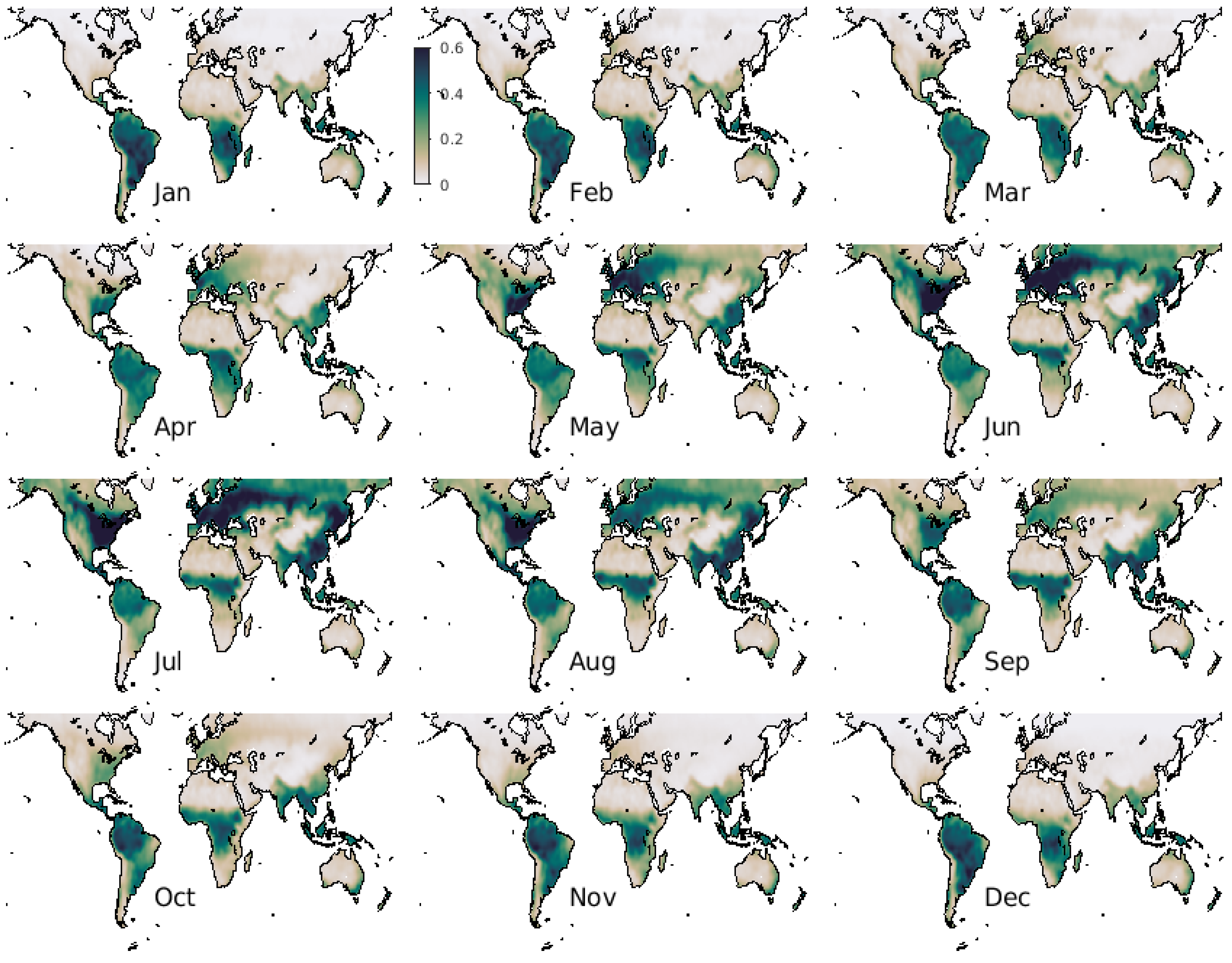
Figure 2.
(left) Global rotated EOF spatial patterns of the first three SIF modes calculated for the 2007–2019 period. (right) Monthly time series (color-shaded, 2007–2019) of the principal components (PCs) associated with the first three global rotated EOF modes. Monthly time series (dashed lines) of correlated climate indices (ENSO for PC1, NAO for PC2, and PDO for PC3) are normalized and superimposed. No time-lag or running mean are performed on these time series. The Pearson correlation coefficient and p-value are given for each time series pair.
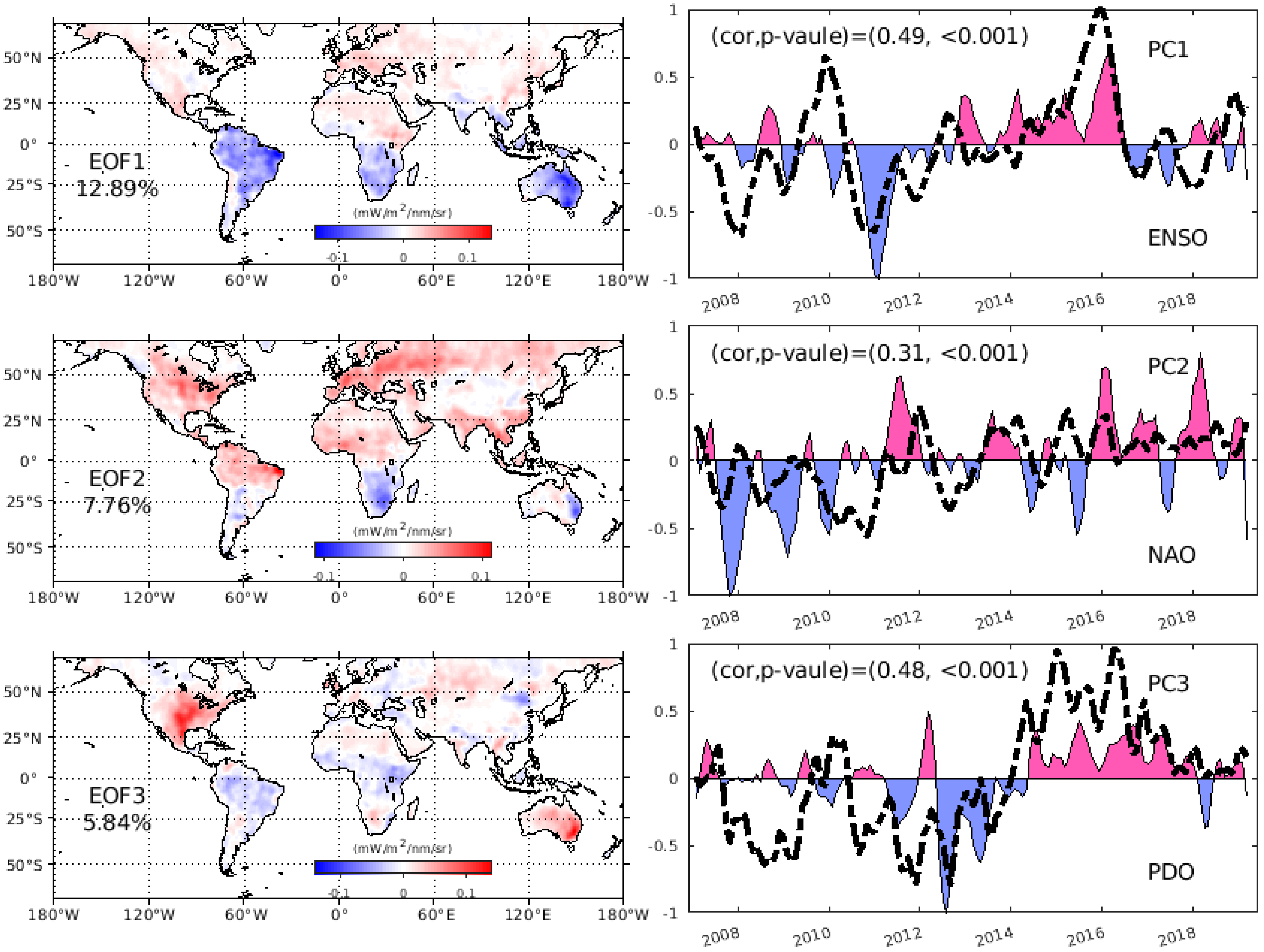
Figure 3.
Difference of annual mean SIF (AMS) between 2011 and 2015, calculated as (AMS2015–AMS2011), highlighting the dramatic changes in SIF between the 2015 El Niño and 2011 La Niña. Unit: mW m−2 sr−1 nm−1.
Figure 3.
Difference of annual mean SIF (AMS) between 2011 and 2015, calculated as (AMS2015–AMS2011), highlighting the dramatic changes in SIF between the 2015 El Niño and 2011 La Niña. Unit: mW m−2 sr−1 nm−1.

Publisher’s Note: MDPI stays neutral with regard to jurisdictional claims in published maps and institutional affiliations. |
© 2022 by the authors. Licensee MDPI, Basel, Switzerland. This article is an open access article distributed under the terms and conditions of the Creative Commons Attribution (CC BY) license (https://creativecommons.org/licenses/by/4.0/).
Share and Cite
MDPI and ACS Style
He, K.; Li, W.; He, R. Variability of Remotely Sensed Solar-Induced Chlorophyll Fluorescence in Relation to Climate Indices. Environments 2022, 9, 121. https://doi.org/10.3390/environments9090121
AMA Style
He K, Li W, He R. Variability of Remotely Sensed Solar-Induced Chlorophyll Fluorescence in Relation to Climate Indices. Environments. 2022; 9(9):121. https://doi.org/10.3390/environments9090121
Chicago/Turabian StyleHe, Katherine, Wenhong Li, and Ruoying He. 2022. "Variability of Remotely Sensed Solar-Induced Chlorophyll Fluorescence in Relation to Climate Indices" Environments 9, no. 9: 121. https://doi.org/10.3390/environments9090121
Note that from the first issue of 2016, this journal uses article numbers instead of page numbers. See further details here.