Predictive Maintenance on the Machining Process and Machine Tool
by
 ,
,
Alberto Jimenez-Cortadi
1,*, 
Itziar Irigoien
2,
Fernando Boto
3,
Basilio Sierra
2 and
German Rodriguez
3 1
TECNALIA, Industry and Transport Division, Leonardo da Vinci 11, 01500 Miñano, Spain
2
Department of Computer Science and Artificial Intelligence, UPV/EHU, 20018 Donostia-San-Sebastian, Spain
3
TECNALIA, Industry and Transport Division, Paseo Mikeletegi 7, 20009 San Sebastian, Spain
*
Author to whom correspondence should be addressed.
Appl. Sci. 2020, 10(1), 224; https://doi.org/10.3390/app10010224
Submission received: 8 November 2019
/
Revised: 18 December 2019
/
Accepted: 19 December 2019
/
Published: 27 December 2019
(This article belongs to the Special Issue New Industry 4.0 Advances in Industrial IoT and Visual Computing for Manufacturing Processes: Volume II)
Abstract
:This paper presents the process required to implement a data driven Predictive Maintenance (PdM) not only in the machine decision making, but also in data acquisition and processing. A short review of the different approaches and techniques in maintenance is given. The main contribution of this paper is a solution for the predictive maintenance problem in a real machining process. Several steps are needed to reach the solution, which are carefully explained. The obtained results show that the Preventive Maintenance (PM), which was carried out in a real machining process, could be changed into a PdM approach. A decision making application was developed to provide a visual analysis of the Remaining Useful Life (RUL) of the machining tool. This work is a proof of concept of the methodology presented in one process, but replicable for most of the process for serial productions of pieces.
1. Introduction
The Oxford Dictionary (2015) defines maintenance as: “the process of preserving a condition or situation or the state of being preserved”. Maintenance is applied mostly to everything, not only in manufacturing processes [1], but also to railways, bikes, cars, computers, etc. Its importance has increased recently while enterprises have noticed the value and cost reduction it implies. In the industrial sector, maintenance has the aim of maintaining a process’s functions over time [2].
At the beginning of the industrial revolution, workers were responsible for equipment maintenance. As the complexity of the machines grew and the maintenance operations increased, enterprises started to include maintenance departments in their business plans. The concept of reliability appeared at the beginning of the 20th Century when maintenance began to be concerned not only with solving failures, but also preventing them. With the arrival of computer science, maintenance strategies had another opportunity to develop more complex models.
Since those beginnings, computational and data analysis technologies have evolved. Not all maintenance methods work for all the processes and assets, but the ones that have been useful have been adapted for new purposes. Currently, the specific needs of each company determine the most appropriate way of performing maintenance to optimize its resources.
Maintenance can be divided into three main types: corrective, preventive, and predictive maintenance. The next paragraphs will describe each of them.
1.1. Corrective Maintenance
This type of maintenance is based on solving the faults that have already happened, which implies it only takes place when the process or machine has a critical halt [3]. Usually, this maintenance provokes a production stop, involving a reduction of production and an increase in costs. The repair time cannot be predicted, nor the degradation or generation of other failures associated with other parts of the process [4]. Because of this, corrective maintenance is used in processes where failures do not have a critical impact on the production.
1.2. Preventive Maintenance
Preventive Maintenance (PM) is a schedule of planned maintenance actions aimed at the prevention of spontaneous breakdowns and failures. It is based on periodic reviews of the system with the aim of preventing failures of it. Despite corrective maintenance, this maintenance is usually applied outside the production time. The objective of this type of employed maintenance is to reduce the number of corrective maintenance actions applied through periodic checks and replacement of worn parts. Ashayeri [5] presented a computer aided planning system for the maintenance of a set of high precision CNC machining centers. Coro et al. [6] presented scheduling inspection of gas turbine welded structures, based on reliability calculations and overhaul findings.
This is demanding maintenance, requiring strict supervision and development of a plan that must be carried out by qualified personnel. In addition, if it is not correctly applied, there will be a breakdown, which provokes a cost in productivity [7].
1.3. Predictive Maintenance
Predictive Maintenance (PdM) is a maintenance type that occurs before breakdown happens. It is based on precise formulas in addition to sensor measurements, and maintenance is performed with the analysis of the measured parameters. The premise of this maintenance is to ensure the maximum interval between repairs and to minimize the cost and number of scheduled maintenance operations (Mobley [8]).
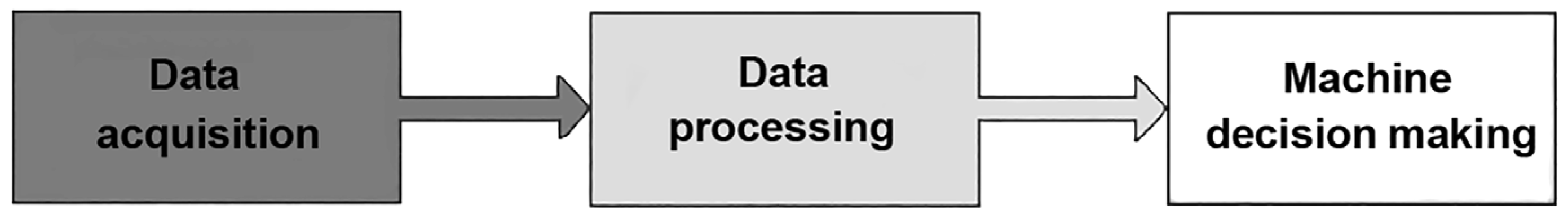
A predictive maintenance program consists of three steps (see Figure 1):
- Data acquisition.
- Data processing.
- Machine decision making.
Although there are monitoring systems dedicated to predicting errors in industrial processes such as Manco et al. [9] exposed for metro doors, the techniques of data analysis and automatic learning have not yet been exploited completely. In this article, some of these techniques will be applied to develop a predictive maintenance. The obtained results will be shown with data extracted from a real process in production. Anticipating how much time is allowed before a failure occurs, which is commonly called the Remaining Useful Life (RUL), is an important task due to the important costs associated with the early replacement of tools [10]. Results show that RUL prediction provides a better accuracy and enables each tool to machine more pieces. Furthermore, the RUL algorithm developed has been deployed with a user visual interface for industrial maintenance purposes, achieving good results also in terms of generalization for other processes. The methodology in this use case is replicable in most of the processes with a serial production of pieces where the machining tool is changed with a certain frequency. Therefore, in this kind of process, the current preventive strategy can be changed by a predictive strategy where the number of pieces for the next tool substitution is predicted.
Section 2 describes the data acquisition step. Section 3 exposes some preprocessing methods. Section 4 presents the machine decision making, where diagnostics and prognostics are explained. Section 5 exposes the particular problem and the developed methodology. Finally, Section 6 concludes about the results and exposes some future works.
2. Data Acquisition
The acquisition of data is the process of collecting and storing data from a physical process in a system, which is essential for the implementation of a predictive maintenance. The data collected in a predictive maintenance program can be classified into two main types: event data and condition monitoring data. While the event data include information about what happened to the asset and which maintenance was applied to it, the condition monitoring data are related to the measurements of the health of the physical asset.Modoni et al. [11] developed a framework for information notification among manufacturing resources. There is a huge variety of signals such as vibrations, acoustics, oil analysis, temperature, pressure, humidity, and climate. In order to collect these data, many sensors have been developed such as ultrasonic sensors, accelerometers, gyroscopes, rain sensors, etc. Many industries are working on improving sensor technologies and computers, which implies an easier way for storing data (Wu et al. [12]).
3. Data Processing
Acquired data are susceptible to presenting some missing, inconsistent, and noise values. Data quality has a great impact on the results obtained by data mining techniques. To improve these results, preprocessing methodologies can be applied. Data preprocessing is one of the most critical steps, which deals with the preparation and transformation of the initial dataset. Data preprocessing methods can be divided into three main categories:
- Data cleaning.
- Data transformation.
- Data reduction.
3.1. Data Cleaning
Raw data are usually incomplete, noisy, or inconsistent, especially event data, which are manually entered. Errors in data may be caused by many factors including human factors to sensor faults, and detecting and removing those errors improve data quality [13]. Dirty data can cause confusion for the mining procedure, and in general, there is no simple way of cleaning. Some techniques are based on human inspection, which usually is helped by some graphical tool. Mean or median values are typically used to pad unknown values with zeros. More sophisticated methods such as regression techniques can be used to estimate missing values. Wei et al. [14] compared eight different methods to recover missing data for mass spectrometry based metabolomics data (zero, half minimum, mean, median, random forest, singular value decomposition, KNN, and QRILC (Quantile Regression Imputation of Left Censored data)). In addition to missing data, noisy values are also a problem for data clearance. The work presented by Libralon et al. [15] proposed the use of clustering methods for noise detection. Data outliers can also be detected by clustering techniques, where similar values are organized into groups. Values that are set outside the clusters will be considered as outliers. Jin et al. [16] applied a one class SVM method for detecting change points in time series data, which would imply a degradation in the system. Maronna et al. [17] proposed another method called the three-sigma edit rule, which was used in Jimenez Cortadi et al. [18] for outlier detection on a radial turning process.
3.2. Data Transformation
Data transformation has the aim of obtaining a more appropriate form of the data for one step further in modeling. Transformations can include standardization, where data are scaled to a small range and make different signals comparable. Smoothing is also applied to data to separate the signal and the noise. For a given dataset, smoothers can be divided as forward and/or backward looking. We will only consider backward looking smoothers, which replace any given observation by a combination of observations at and before it. A short overview of different smoothing methods can be found in [19]. Yahyaoui and Al-Daihani [20] suggested a novel Symbolic Aggregate approXimation (SAX) and compared it to the standards, obtaining better results for time series classification. Smoothing techniques also include regressions and clustering.
3.3. Data Reduction
Having a considerable amount of data can be an issue for machine decision making in terms of having a big computational cost. As the number of data increases, the time spent by the hardware will also increase. To maintain the computational cost while the amount of data is sufficient, some methodologies have been developed over the years. The best known one is principal component analysis (Jolliffe and Cadima [21]). This method is based on combining input features linearly to obtain new ones, which are linearly independent of each other and maintain as much of the original information as possible.
Other data reduction methods are recursive feature elimination [22] and t-distributed Stochastic Neighbor Embedding (t-SNE) applied by Pouyet et al. [23] to provide a non-linear representation of spectral features in a lower 2D space. More feature selection techniques were presented in Guyon and Elisseeff [24]. Wang et al. [25] proposed a dimensionality reduction method using global characteristics such as seasonality, trend, periodicity, and skew for feature selection before using a Self-Organization Map (SOM).
4. Machine Decision Making
This is the last step in the maintenance decision, which can be divided into two main categories: diagnostics and prognostics. Diagnostics focuses on detection, identification, and isolation of faults when they occur, while prognostics pretends to predict failures before they happen and is related to predictive maintenance. Diagnostics and prognostics are complementary in that diagnostics adds new information from the process. This information enables going from an unsupervised problem to a supervised one. A supervised model is always easier to develop and has greater accuracy, which implies a better prognostics model.
4.1. Diagnostics
Fault diagnosis is the process of tracing a fault by identifying its symptoms, applying knowledge, and analyzing test results [26]. Accurate diagnosis consists of detection of the faults and determination and estimation of the size and nature of the location. Fault diagnosis requires advanced algorithms such as Machine Learning (ML) techniques, which are increasingly applied in not only the industrial sector, such as manufacturing, aerospace, and automotive, but also in business, finance, and science. The most frequently employed algorithms in the industrial sector are: linear regression, random forest (Mattes et al. [27]), Markov models (Cartella et al. [28]), artificial neural networks (Farokhzad et al. [29], Kanawaday and Sane [30], Li et al. [31]), and support vector machines (Tyagi [32], Widodo and Yang [33]). Diez-Olivan et al. [34] provided an overview of the algorithms employed in the industrial sector for diagnosis.
These techniques can also be applied to detect changes in the system behavior as an indication of the beginning of malfunctions, which is called concept drift (Tsymbal [35]). Winkler et al. [36] applied a sliding window symbolic regression model for concept drift detection in dynamic systems. Klinkenberg and Joachims [37] detected concept drift by applying SVM and adjusting the window size to minimize the estimated generalization error. Zhukov et al. [38] detected concept drift on publicly available benchmark datasets with the random forest technique.
4.2. Prognostics
Predicting the time when a system or a component will no longer perform properly is referred to as prognostics (Galar and Kumar [26]). Prognostics predict future performance given the current machine status and past operation profile, which is an important task to know if the process will maintain its functions over time [2]. Two main prediction types can be found in machine prognostics: on the one hand, predicting RUL, which is explained in Section 1; on the other hand, predicting the probability that a machine has to keep on working without a failure up to some time [39]. Pham et al. [40] applied an ARMA model to vibration data for machine state forecast. Khelif et al. [41] used a Support Vector Regressor (SVR) to predict RUL. Djeziri et al. [42] provided a similar methodology to the one explained in this work where a fault prognosis was developed by a preprocessing method and an extrapolation of the previous values to predict RUL. Other examples in industry can also be found in [34].
5. Case Study
In this section, an application of predictive maintenance is exposed on a real machining process. The main goals of this study are to increase tool life and to identify whether there is a concept drift. These aims will be achieved applying some ML methods for RUL prediction and concept drift detection.
5.1. Industrial Process
The experiments were conducted on a CNC turning center with two tool posts, which could be moved on two axes independently with longitudinal and cross-feed movement. The cutting tool holder used was a C3-MTJNR-22040-16 equipped with a TNMG160408-PF insert for the external surface and a special tool holder equipped with a WNMG060408-PM insert for the inner diameter. During the machining process, the rotating revolutions were set to 1800 rpm. The current maintenance strategy applied was a very conservative method to change the machining tool when the specific number of pieces machined was higher than a threshold. Therefore, a predictive strategy was very interesting for this kind of processes.
5.2. Acquisition
During the turning process, from December 2017 until May 2019, several measurement were recorded, which provided information about how the machine was working. These Condition Monitoring (CM) signals were obtained with a 5Hz frequency. Although several signals were acquired, the final state of the tool (piece quality) was not measured. The acquired signals, such as spindle load, piece number, and tool position, were recorded as a collection of observations made sequentially through time, which are known as time series. In this case, experts in the process suggest the spindle load signal to be studied, while other signals are useful for segmentation and characterization. The spindle load represents machine effort and is the more critical signal over all the sensorized ones. As a result of this acquisition step, around 1100 series and 550,000 pieces were stored for further analysis. The technology applied for monitoring data is shown in Figure 2. The monitoring system (data recorder) was connected to the machine tool, which recorded a database accessible via the Internet and had different interfaces. The machine tool data recorder worked on the same principle as the black box on a flight deck. It communicated with the control unit of the machine and some independent sensors, in order to retrieve targeted data. The data recorder was able to communicate with Computer Numerical Control (CNC). Its design only permitted the recording device to communicate with the interface of the control unit, in order to access the control memory in read-only mode. At no point would it therefore disturb the execution of the program. All monitored data were configured by default to be stored in a secured remotely accessible database. The connection between the database and the machine tool data recorder was done through an Ethernet connection.
5.3. Data Processing
As explained before, there is a huge amount of possibilities, and in this work, reduction, cleaning, and transformation were applied.
Data reduction is based on extracting characteristics from the original signal to have a smaller amount of data, so the computational cost is reduced and the data are clearer. The first step is to cut the signal so that we can observe the spindle load evolution for each tool. To achieve this aim, the signal, which represents the number of pieces machined, was used, since the piece number is restarted when the tool changes. In addition to this reduction, each machined piece was characterized by the highest spindle load value recorded during its machined time, which was suggested by the expert.
The obtained characterization (see Figure 3) appeared to have some outliers, which must be removed. To achieve this aim, the three-sigma edit rule technique was applied [17]. This method is based on the difference between each value and the median of the signal:
where S is the full spindle load signal and p is the number of machined pieces. The robust three-sigma edit rule establishes that the observation is an outlier if: , where r is a threshold value. In this case, is set with expert supervision.
As a second step, and once the outliers were removed, we transformed the series by a smoothing method. The Savitzky–Golay [43] and Wiener [44] smoothing methods were tested. Savitzky–Golay is a smoothing method based on moving average value. In particular, in this work, being the value of the series in the machined piece or point, Savitzky–Golay determined a new by calculating a cubic polynomial with values around the point p:
where is the coefficient associated with the point on the polynomial approximation.
The Savitzky–Golay filter was the transformation that obtained a better visualization of the signal and enabled detecting the main trends on the series, which was the main issue of this part of the study.
Taking into account that some of the signals had different behaviors (see Figure 4), a final step in data processing was carried out. This reduction was obtained by applying an iterative clustering method. This methodology provided a two group classification based on K-means on each iteration, and if one of the groups had less than 10% of the signals, those signals were not considered as normal or regular behavior. The One Class-Support Vector Machine (OC-SVM) [45] classification method was applied as a validation of the clustering method mentioned above. This method generated a hyperplane where the normal behavior was found and separated those abnormal values. Validation was obtained successfully. Finally, with the selected regular series, machine learning techniques were applied to estimate the RUL.
5.4. Concept Drift Detection
Having such an amount of data acquired over a long time made it necessary to identify whether there was a concept drift or not in order to select the appropriate signals for RUL estimation. The concept drift search was done to identify whether the machine suffered some wear during this time. We sought two different types of concept drift. On the one hand, concept drift detection for the hole machine was suggested. This approximation was done taking all the maximum spindle values for every machined piece and a linear regressor, and no tendency over time was detected, which enabled us to use all the signals for the RUL detection. This could be due to the big machine lifetime compared to the period we observed. On the other hand, a concept drift for each tool was sought. This detection was done by studying the evolution of the errors derived from regression models built for each series. Some values of the series were selected at random, and the predicted and observed values were compared to the obtained error. If this error (Mean Squared Error MSE (Equation (1))) grew for each forecasting piece, it would indicate that there was a concept drift. In the case we studied, no concept drift was detected for the tool.
where is the observed series and is the predicted series.
5.5. Decision Making Application for RUL Estimation
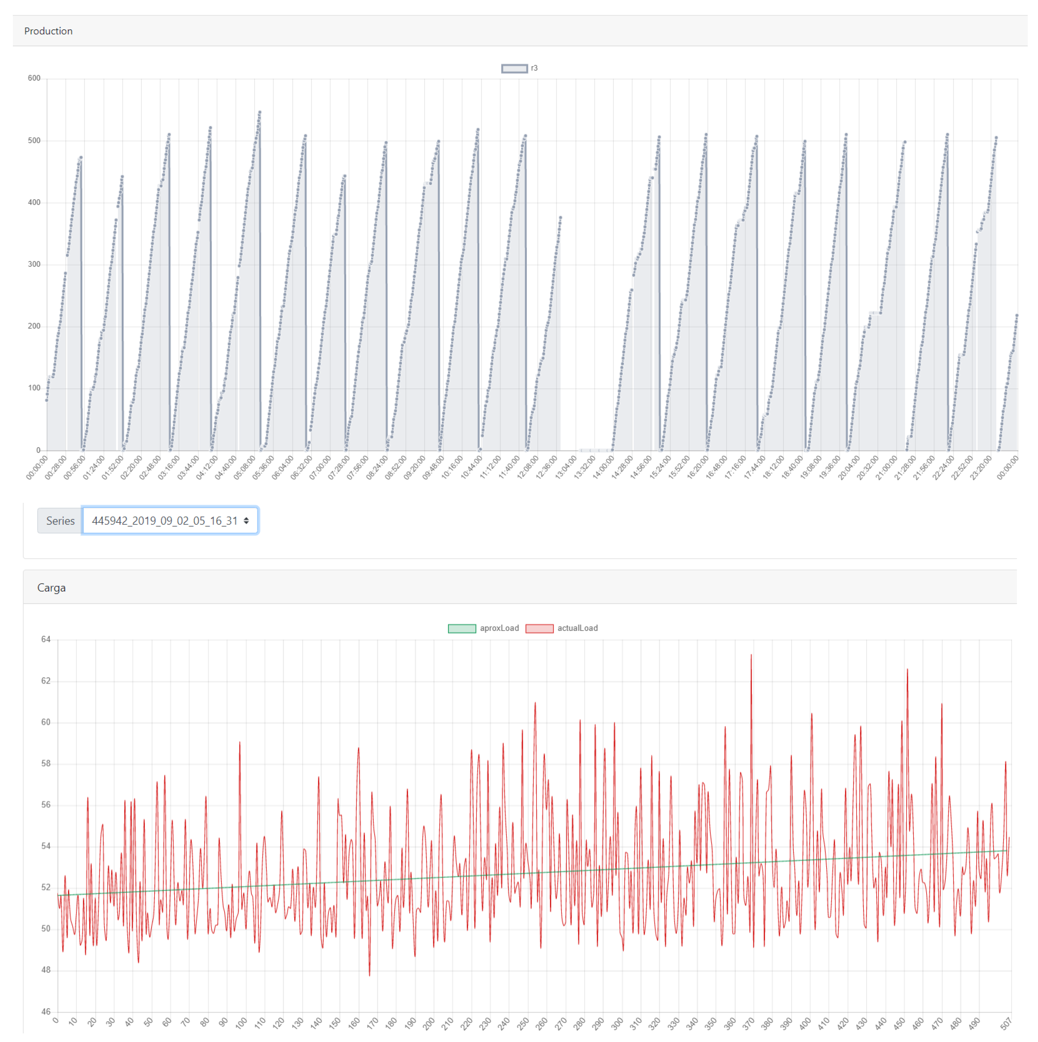
Customers always want to obtain some digital device that enables seeing the online state of the process. Therefore, we worked on models to be implemented in real time on the machine. Approximation was made with linear and quadratic regressions. In similar mechanical processes, Cortadi et al. [46] showed that quadratic approximation was the one that fit best. Nevertheless, in this particular machining process, the second order curve introduced some physical incoherence in some of the series, and the first order approximation gave better results. This approximation has been developed, and currently, it is accessible at the machine itself (see Figure 5). Based on the data acquisition platform (see Figure 5), it provided a visualization of the acquired signals along the machining process. This visualization could be made not only for historical data (from the database associated with the tool), but also for actual series. Moreover, as can be seen in Figure 5, an estimation of the RUL in terms of the amount of remaining pieces the tool could still machine safely is given, and this value was obtained by applying a linear regression to the pieces machined until that point and determining when the line would go past a threshold. Also shown are the number of pieces machined during a whole day (Figure 5, top) and a particular series with a linear regression (Figure 5, bottom), which provided the aforementioned estimation before the replacement of the tool was required. This application offered a means to have a predictive maintenance instead of the preventive maintenance used before.
5.6. Remaining Useful Life Assessment
For an offline prediction of the spindle load, other models were applied. These models were: ARIMA [47], Gradient Boosting (GB) [48], Random Forest (RF) [49], and Recurrent Neural Network (RNN) [50].
With all the regular series identified in the data processing step, a mean series was built. To evaluate the predictive ability of the models, the training set was made of the first part of the series and the test with the last p values: 10, 20, 30, 40, and 50 values of the series. The ARIMA model was generated with the series itself, while GB, RF, and RNN were developed with the input of the value of the series on each instant t and the previous 9 , so that 10 values were taken into account for prediction. In all the models, the output of the model was the spindle load of the instances from . The obtained results are shown in Table 1 and present the MSE of the p predicted values against the measured ones. Notice that the values were multiplied by .
The results were shown to be good, and in Figure 6, the prediction obtained by each model and the real signal (blue) can be seen. This figure was made with 20 test pieces, while all tested values had similar results. It was shown to have good accuracy in the short term, but the strength was lost in the long term, which implied that an extension of the machining process could be done, while an RUL value could only be suggested once the process was near the threshold.
On the other hand, the ARIMA, GB, RF, and RNN models we obtained for the mean regular series were applied on each series separately. Some random series were taken for the validation of the models in order to define if the machining process could be extended in time. As long the machine had a preventive maintenance, these methods were demonstrated to enable the tool to increase the number of pieces machined at least by 20 pieces more; this value is determined in Table 1 as the more accurate one. The spindle load of 115 series was studied, and it could be concluded that for 113 of them, the tool’s lifetime could be extended. For only two of the series, the threshold was passed, and an earlier maintenance was suggested.
In Figure 7, a flowchart representing the main steps applied on this methodology is provided. First, the spindle load acquisition data are presented. These data needed to be discretized before a characterization was applied. This discretization is shown in Figure 7b. The characterization was based on expert knowledge, and each piece’s maximum value was extracted. For each tool, a new time series was developed (see Figure 7c). The obtained series were cleaned and smoothed for better prediction, and future value prediction was developed. Figure 7d shows the ARIMA approach of one series, and Figure 7e presents the comparison between all the machine learning methods applied in this work.
Since this work provided a customized solution for a real problem in a factory, as far as we know, there are no works from which comparative results to the solution we found could be obtained. Nevertheless, some similarities were found with [42]. These similarities were:
- RUL estimation.
- Application in a discrete machining process.
- Characterization of the signal acquired (Health Indicator (HI)).
Although the goal and the main steps were similar, there were some differences:
Even if these two works cannot be compared numerically, it can be said that the methodology applied in this work was coherent with the one developed by Djeziri et al. [42]. The mentioned differences provided a more complex methodology, which enabled more accurate and robust predictions.
6. Conclusions and Future Work
This study achieved two different goals: First was an application developed to visualize the RUL in a machining process that was based on a linear regression model, which was actually based on the production, providing a predictive maintenance. The application was updated each time a new machining series began. Second was to obtain more accurate results to predict the RUL for comparison. Although accuracy was gained, the complexity of the models made their implementation more difficult in the production machine.
In this work, a methodology that could be applied not only in this process, but also in most of the processes for serial production of pieces was provided. Similar processes will be studied with this approach to validate this methodology with some limitations. The signal considered to predict the RUL was the spindle load, but it is our aim to include other signals and study their contribution to obtain a better explanation of the process and more accurate RUL prediction. Furthermore, as the spindle of the process was made of two different tools, two different RUL predictions needed to be done, each one for each tool. Finally, we are working to increase the frequency acquisition of the signals. This increase would improve the characterization of the signal and hence enable recording more features, which could explain the process better and develop more accurate models.
Author Contributions
Conceptualization, A.J.-C. and G.R.; methodology, A.J.-C. and F.B.; software, A.J.-C. and I.I.; validation, A.J.-C., I.I. and B.S.; formal analysis, F.B.; investigation, A.J.-C.; resources, G.R.; data curation, A.J.-C.; writing–original draft preparation, A.J.-C.; writing–review and editing, A.J.-C., F.B. and I.I.; visualization, A.J.-C.; supervision, B.S.; project administration, G.R.; funding acquisition, G.R. All authors have read and agreed to the published version of the manuscript.
Funding
This research received no external funding
Acknowledgments
The work was performed as a part of the INSIGHTSproject within the HAZITEKprogram of the Economic and Infrastructure Department of the Basque Government.
Conflicts of Interest
The authors declare no conflict of interest.
References
- Cimino, C.; Negri, E.; Fumagalli, L. Review of digital twin applications in manufacturing. Comput. Ind. 2019, 113, 103130. [Google Scholar] [CrossRef]
- Galar, D.; Palo, M.; Van Horenbeek, A.; Pintelon, L. Integration of disparate data sources to perform maintenance prognosis and optimal decision making. Insight-Non-Destr. Test. Cond. Monit. 2012, 54, 440–445. [Google Scholar] [CrossRef]
- Vathoopan, M.; Johny, M.; Zoitl, A.; Knoll, A. Modular fault ascription and corrective maintenance using a digital twin. IFAC-PapersOnLine 2018, 51, 1041–1046. [Google Scholar] [CrossRef]
- Swanson, E.B. The dimensions of maintenance. In Proceedings of the 2nd International Conference on Software Engineering, Wuhan, China, 13–15 January 1976; pp. 492–497. [Google Scholar]
- Ashayeri, J. Development of computer-aided maintenance resources planning (CAMRP): A case of multiple CNC machining centers. Robot. -Comput.-Integr. Manuf. 2007, 23, 614–623. [Google Scholar] [CrossRef]
- Coro, A.; Abasolo, M.; Aguirrebeitia, J.; Lopez de Lacalle, L. Inspection scheduling based on reliability updating of gas turbine welded structures. Adv. Mech. Eng. 2019, 11, 1687814018819285. [Google Scholar] [CrossRef] [Green Version]
- Vilarinho, S.; Lopes, I.; Oliveira, J.A. Preventive maintenance decisions through maintenance optimization models: A case study. Procedia Manuf. 2017, 11, 1170–1177. [Google Scholar] [CrossRef]
- Mobley, R.K. An Introduction to Predictive Maintenance; Elsevier: Amsterdam, The Netherlands, 2002. [Google Scholar]
- Manco, G.; Ritacco, E.; Rullo, P.; Gallucci, L.; Astill, W.; Kimber, D.; Antonelli, M. Fault detection and explanation through big data analysis on sensor streams. Expert Syst. Appl. 2017, 87, 141–156. [Google Scholar] [CrossRef]
- Aramesh, M.; Attia, M.; Kishawy, H.; Balazinski, M. Estimating the remaining useful tool life of worn tools under different cutting parameters: A survival life analysis during turning of titanium metal matrix composites (Ti-MMCs). CIRP J. Manuf. Sci. Technol. 2016, 12, 35–43. [Google Scholar] [CrossRef]
- Modoni, G.E.; Trombetta, A.; Veniero, M.; Sacco, M.; Mourtzis, D. An event-driven integrative framework enabling information notification among manufacturing resources. Int. J. Comput. Integr. Manuf. 2019, 32, 241–252. [Google Scholar] [CrossRef]
- Wu, R.; Huang, L.; Zhou, H. RHKV: An RDMA and HTM friendly key–value store for data-intensive computing. Future Gener. Comput. Syst. 2019, 92, 162–177. [Google Scholar] [CrossRef]
- Lenzerini, M. Data Integration: A Theoretical Perspective. In Proceedings of the the 21st ACM SIGMOD-SIGACT-SIGART Symposium on Principles of Database Systems (PODS02), Madison, WI, USA, 3–5 June 2002. [Google Scholar]
- Wei, R.; Wang, J.; Su, M.; Jia, E.; Chen, S.; Chen, T.; Ni, Y. Missing Value Imputation Approach for Mass Spectrometry-Based Metabolomics Data. Sci. Rep. 2018, 8, 663. [Google Scholar] [CrossRef] [PubMed] [Green Version]
- Libralon, G.L.; de Leon Ferreira, A.C.P.; Lorena, A.C. Pre-processing for noise detection in gene expression classification data. J. Braz. Comput. Soc. 2009, 15, 3–11. [Google Scholar] [CrossRef] [Green Version]
- Jin, B.; Chen, Y.; Li, D.; Poolla, K.; Sangiovanni-Vincentelli, A. A One-Class Support Vector Machine Calibration Method for Time Series Change Point Detection. arXiv 2019, arXiv:1902.06361. [Google Scholar]
- Maronna, R.; Martin, R.D.; Yohai, V. Robust Statistics; John Wiley & Sons: Chichester, UK, 2006. [Google Scholar]
- Jimenez Cortadi, A.; Irigoien, I.; Boto, F.; Sierra, B.; Suarez, A.; Galar, D. A statistical data-based approach to instability detection and wear prediction in radial turning processes. Eksploatacja i Niezawodnosc 2018, 20, 405–412. [Google Scholar] [CrossRef]
- Mills, T.C. Applied Time Series Analysis: A Practical Guide to Modeling and Forecasting; Academic Press: Cambridge, MA, USA, 2019. [Google Scholar]
- Yahyaoui, H.; Al-Daihani, R. A novel trend based SAX reduction technique for time series. Expert Syst. Appl. 2019, 130, 113–123. [Google Scholar] [CrossRef]
- Jolliffe, I.T.; Cadima, J. Principal component analysis: A review and recent developments. Philos. Trans. R. Soc. A 2016, 374, 20150202. [Google Scholar] [CrossRef]
- Darst, B.F.; Malecki, K.C.; Engelman, C.D. Using recursive feature elimination in random forest to account for correlated variables in high dimensional data. BMC Genet. 2018, 19, 65. [Google Scholar] [CrossRef] [Green Version]
- Pouyet, E.; Rohani, N.; Katsaggelos, A.K.; Cossairt, O.; Walton, M. Innovative data reduction and visualization strategy for hyperspectral imaging datasets using t-SNE approach. Pure Appl. Chem. 2018, 90, 493–506. [Google Scholar] [CrossRef]
- Guyon, I.; Elisseeff, A. An introduction to variable and feature selection. J. Mach. Learn. Res. 2003, 3, 1157–1182. [Google Scholar]
- Wang, X.; Wirth, A.; Wang, L. Structure-based statistical features and multivariate time series clustering. In Proceedings of the Seventh IEEE International Conference on Data Mining (ICDM 2007), Omaha, NE, USA, 28–31 October 2007; pp. 351–360. [Google Scholar]
- Galar, D.; Kumar, U. EMaintenance: Essential Electronic Tools for Efficiency; Academic Press: Cambridge, MA, USA, 2017. [Google Scholar]
- Mattes, A.; Schöpka, U.; Schellenberger, M.; Scheibelhofer, P.; Leditzky, G. Virtual equipment for benchmarking predictive maintenance algorithms. In Proceedings of the 2012 Winter Simulation Conference (WSC), Berlin, Germany, 9–12 December 2012; pp. 1–12. [Google Scholar]
- Cartella, F.; Lemeire, J.; Dimiccoli, L.; Sahli, H. Hidden semi-Markov models for predictive maintenance. Math. Probl. Eng. 2015, 2015, 278120. [Google Scholar] [CrossRef] [Green Version]
- Farokhzad, S.; Ahmadi, H.; Jaefari, A.; Abad, M.; Kohan, M.R. Artificial neural network based classification of faults in centrifugal water pump. J. Vibroeng. 2012, 14, 1734–1744. [Google Scholar]
- Kanawaday, A.; Sane, A. Machine learning for predictive maintenance of industrial machines using iot sensor data. In Proceedings of the 2017 8th IEEE International Conference on Software Engineering and Service Science (ICSESS), Beijing, China, 20–22 November 2017; pp. 87–90. [Google Scholar]
- Li, Z.; Wang, Y.; Wang, K.S. Intelligent predictive maintenance for fault diagnosis and prognosis in machine centers: Industry 4.0 scenario. Adv. Manuf. 2017, 5, 377–387. [Google Scholar] [CrossRef]
- Tyagi, C.S. A comparative study of SVM classifiers and artificial neural networks application for rolling element bearing fault diagnosis using wavelet transform preprocessing. Neuron 2008, 1, 309–317. [Google Scholar]
- Widodo, A.; Yang, B.S. Support vector machine in machine condition monitoring and fault diagnosis. Mech. Syst. Signal Process. 2007, 21, 2560–2574. [Google Scholar] [CrossRef]
- Diez-Olivan, A.; Del Ser, J.; Galar, D.; Sierra, B. Data fusion and machine learning for industrial prognosis: Trends and perspectives towards Industry 4.0. Inf. Fusion 2019, 50, 92–111. [Google Scholar] [CrossRef]
- Tsymbal, A. The problem of concept drift: Definitions and related work. Comput. Sci. Dep. Trinity Coll. Dublin 2004, 106, 58. [Google Scholar]
- Winkler, S.M.; Affenzeller, M.; Kronberger, G.; Kommenda, M.; Burlacu, B.; Wagner, S. Sliding window symbolic regression for detecting changes of system dynamics. In Genetic Programming Theory and Practice XII; Springer: Berlin/Heidelberg, Germany, 2015; pp. 91–107. [Google Scholar]
- Klinkenberg, R.; Joachims, T. Detecting concept drift with support vector machines. In Proceedings of the Seventeenth International Conference on Machine Learning, Stanford, CA, USA, 29 June 29–2 July 2000; pp. 487–494. [Google Scholar]
- Zhukov, A.V.; Sidorov, D.N.; Foley, A.M. Random forest based approach for concept drift handling. In Proceedings of the International Conference on Analysis of Images, Social Networks and Texts, Yekaterinburg, Russia, 7–9 April 2016; pp. 69–77. [Google Scholar]
- Goyal, D.; Pabla, B. Condition based maintenance of machine tools—A review. CIRP J. Manuf. Sci. Technol. 2015, 10, 24–35. [Google Scholar] [CrossRef]
- Pham, H.T.; Yang, B.S.; Tran, V.T.; Yang, B.-S. A hybrid of nonlinear autoregressive model with exogenous input and autoregressive moving average model for long-term machine state forecasting. Expert Syst. Appl. 2010, 37, 3310–3317. [Google Scholar] [CrossRef] [Green Version]
- Khelif, R.; Chebel-Morello, B.; Malinowski, S.; Laajili, E.; Fnaiech, F.; Zerhouni, N. Direct remaining useful life estimation based on support vector regression. IEEE Trans. Ind. Electron. 2017, 64, 2276–2285. [Google Scholar] [CrossRef]
- Djeziri, M.; Ananou, B.; Ouladsine, M.; Pinaton, J.; Nguyen, T.-B.-L. Fault prognosis for discrete manufacturing processes. IFAC Proc. Vol. 2014, 47, 8066–8072. [Google Scholar]
- Savitzky, A.; Golay, M.J. Smoothing and differentiation of data by simplified least squares procedures. Anal. Chem. 1964, 36, 1627–1639. [Google Scholar] [CrossRef]
- Extrapolation, I. Smoothing of Stationary Time Series; Martino Fine Books: New York, NY, USA, 1949. [Google Scholar]
- Hejazi, M.; Singh, Y.P. One-class support vector machines approach to anomaly detection. Appl. Artif. Intell. 2013, 27, 351–366. [Google Scholar] [CrossRef]
- Cortadi, A.J.; Boto, F.; Irigoien, I.; Sierra, B.; Suarez, A. Instability Detection on a Radial Turning Process for Superalloys. In Proceedings of the International Joint Conference SOCO17-CISIS17-ICEUTE17, León, Spain, 6–8 September 2017; pp. 247–255. [Google Scholar]
- Box, G.E.; Jenkins, G.M.; Reinsel, G.C.; Ljung, G.M. Time Series Analysis: Forecasting and Control; John Wiley & Sons: Hoboken, NJ, USA, 2015. [Google Scholar]
- Breiman, L. Arcing the Edge; Technical Report 486; Statistics Department, University of California: Berkeley, CA, USA, 1997. [Google Scholar]
- Prinzie, A.; Van den Poel, D. Random multiclass classification: Generalizing random forests to random mnl and random nb. In Proceedings of the International Conference on Database and Expert Systems Applications, Regensburg, Germany, 3–7 September 2007; pp. 349–358. [Google Scholar]
- Connor, J.; Atlas, L. Recurrent neural networks and time series prediction. In Proceedings of the IJCNN-91-Seattle International Joint Conference on Neural Networks, Seattle, WA, USA, 8–12 July 1991; Volume 1, pp. 301–306. [Google Scholar]
Figure 1.
Steps followed to develop a predictive maintenance.

Figure 2.
Data acquisition platform flows and architecture.

Figure 3.
One time series spindle load before outlier removal.

Figure 4.
Time series after smoothing transformation in a period of time.

Figure 5.
Application integrated at the machine showing the Remaining Useful Life (RUL) for the actual working tool.
Figure 5.
Application integrated at the machine showing the Remaining Useful Life (RUL) for the actual working tool.

Figure 6.
Prediction for the mean series of each regressor.

Figure 7.
Flowchart of the main steps of the methodology exposed in this work.


Table 1.
Mean MSE values for each method for each different number of test pieces (multiplied by ). GB, Gradient Boosting.
Table 1.
Mean MSE values for each method for each different number of test pieces (multiplied by ). GB, Gradient Boosting.
| Test Pieces | ARIMA | GB | RF | RNN |
|---|---|---|---|---|
| 10 | 3.668 | 3.832 | 4.050 | 4.256 |
| 20 | 2.832 | 3.227 | 2.891 | 3.524 |
| 30 | 3.166 | 3.833 | 3.325 | 3.885 |
| 40 | 3.909 | 3.489 | 3.121 | 3.756 |
| 50 | 3.791 | 3.899 | 4.065 | 4.002 |
© 2019 by the authors. Licensee MDPI, Basel, Switzerland. This article is an open access article distributed under the terms and conditions of the Creative Commons Attribution (CC BY) license (http://creativecommons.org/licenses/by/4.0/).
Share and Cite
MDPI and ACS Style
Jimenez-Cortadi, A.; Irigoien, I.; Boto, F.; Sierra, B.; Rodriguez, G. Predictive Maintenance on the Machining Process and Machine Tool. Appl. Sci. 2020, 10, 224. https://doi.org/10.3390/app10010224
AMA Style
Jimenez-Cortadi A, Irigoien I, Boto F, Sierra B, Rodriguez G. Predictive Maintenance on the Machining Process and Machine Tool. Applied Sciences. 2020; 10(1):224. https://doi.org/10.3390/app10010224
Chicago/Turabian StyleJimenez-Cortadi, Alberto, Itziar Irigoien, Fernando Boto, Basilio Sierra, and German Rodriguez. 2020. "Predictive Maintenance on the Machining Process and Machine Tool" Applied Sciences 10, no. 1: 224. https://doi.org/10.3390/app10010224
Note that from the first issue of 2016, this journal uses article numbers instead of page numbers. See further details here.