Performance Analysis of Maximal Risk Evaluation Formulas for Spectrum-Based Fault Localization

Abstract

The effectiveness analysis of risk evaluation formulas has become a significant research area in spectrum-based fault localization (SBFL). The risk evaluation formula is designed and widely used to evaluate the likelihood of a program spectrum to be faulty. There are numerous empirical and theoretical studies to investigate and compare the performance between sixty risk evaluation formulas. According to previous research, these sixty risk evaluation formulas together form a partially ordered set. Among them, nine formulas are maximal. These nine formulas can further be grouped into five maximal risk evaluation formula groups so that formulas in the same group have the same performance. Moreover, previous research showed that we cannot theoretically compare formulas across these five maximal formula groups. However, experimental data “suggests” that a maximal formula in one group could outperform another one (from a different group) more frequently, though not always. This inspired us to further investigate the performance between any two maximal formulas in different maximal formula groups. Our approach involves two major steps. First, we propose a new condition to compare between two different maximal formulas. Based on this new condition, we present five different scenarios under which a formula performs better than another. This is different from the condition suggested by the previous theoretical study. We performed an empirical study to compare different maximal formulas using our condition. Our results showed that among two maximal risk evaluation formulas, it is feasible to identify one that can outperform the others more frequently.

1. Introduction

Spectrum-based fault localization (SBFL) [1,2] is an important technique aiming to locate the most possible faulty statements during software testing and debugging processes, which are time consuming, resource intensive, and expensive due to the ever increasing scale and complexity of software [3]. To determine the suspicious area in a faulty program, SBFL utilizes the concept of program spectrum. Loosely speaking, a program spectrum is a “certain entity” of the program under debugging together with the execution information, such as testing results and coverage information, with respect to a test suite. The program entity can be of any granularity [1], ranging from a simple statement to a certain basic block. The purpose of SBFL is to identify which program spectrum, actually the program entity contained in the spectrum, is more likely to have faults. For SBFL to be possible, all information related to program spectra have to be collected during the testing of the program. Based on these collected information, debugger uses a risk evaluation formula to calculate the risk values of all program spectra and then ranks these risk values in descending order because the risk evaluation formula has been designed in such a way that the higher the risk value of a program spectrum is, the more likely the program spectrum contains faults. The program debugger then inspects the program spectrum ranking list from top to bottom, and those program spectra with high risk values are regarded as the likely faulty areas [4]. Since there are many different risk evaluation formulas proposed in the research literature and different formulas may give rise to different risk values, which lead to different ranking orders, and hence, different “potential” faulty areas, it is necessary to find the most effective formula to “best” locate the faulty program entity.

There are both empirical and theoretical researches on studying the effectiveness of different risk evaluation formulas. For example, empirical investigations have been used to compare the performances of different risk evaluation formulas [2,4,5,6,7,8,9,10]. However, the empirical investigation can never be sufficient and fair enough to compare formulas because of different experimental setups and factors affecting the results.

Theoretical approaches have been proposed to analyze the effectiveness of risk evaluation formulas [11,12,13,14,15,16,17]. Detailed definitions and discussions on their work are in Section 2.2. Theoretical analysis proves that (a) there are five groups of maximal formulas [14,17]; (b) formulas within the same group have the same performance [14]; and (c) no formula from one of these groups always comes out ahead of a formula from another group [18]. However, it is possible that one formula from one group more frequently (though not always) comes out ahead of a formula from another group. It is too difficult to use a theoretical analysis to show which formula more frequently comes out ahead of another formula, because there are many possible variations. Therefore, we adopted an empirical analysis to see which formula more frequently comes out ahead of another formula.

This then led us to investigate the following research questions

• For any two maximal formulas from different maximal formula groups, which one can perform better than another one more frequently?
• Is there a maximal formula group that can always perform better than other maximal formula groups more frequently?

Please note that previous research has shown that there are five maximal formula groups and the maximal formulas from the same maximal group have the same performance. Hence, we only need to pick one maximal formula from each of these five groups and compare them in a pairwise manner. Hence, we have 10 such comparisons. We performed an empirical study on 11 small to medium sized C programs ranging from 135 to 9932 source lines of code with an average of 3137.8. We present our findings in this work.

The primary contributions of this paper are summarized as follows:

(1)

We performed an empirical study to compare between any two maximal risk evaluation formulas, each from a different maximal formula group.

(2)

We propose using a new condition to compare between two risk evaluation formulas. This condition is different from other similar empirical and theoretical studies. We use the expected location of the “faulty” statement to compare between the formulas, whereas previous studies used the exact location for comparison.

(3)

We present and discuss five different scenarios that could lead to the conclusion that one maximal formula can perform better than another maximal formula more frequently using our condition. However, when using the “exact location” condition as in the previous study, these scenarios could not be easily discovered or discussed.

The remainder of this paper is organized as follows. Section 2 introduces the background of SBFL and the maximal risk evaluation formula groups. Section 3 proposes a new condition to compare between two risk evaluation formulas. It also discusses the five scenarios to cover all possible cases that one formula outperforms another one. Section 4 discusses our empirical study, its results, and its threats to validity. Section 5 describes the related work on the effectiveness of SBFL techniques. Finally, Section 6 concludes the paper and discusses future work.

2. Background

2.1. Spectrum-Based Fault Localization (SBFL)

Spectrum-based fault localization (SBFL) uses two significant pieces of information to help localize faults, if any, in a program during the software testing and debugging processes. The first piece of information is the testing result of the program with respect to a test suite. It basically indicates whether a program passes or fails on each individual test case. The second piece of information is the program spectrum, which contains the information about a program entity (e.g., statement, branch or basic block) and its coverage information, such as whether it has been executed or not; how many test cases that execute or do not execute in the program entity such that the program passes; and how many test cases that execute or do not execute in the program entity such that the program fails [3]. The program spectrum information, together with the test results, provide a behavioral signature for program execution with respect to a test suite [1]. It also describes the characterized information of the program entities obtained from program runtime profiling when the program executes on the test suite. From software testing perspective, a program entity could be a statement, branch, path, function, or basic block, among which statement is the most widely used because of its analysis simplicity [19]. The characterized information of a program entity could be the number of times that the program entity has been executed, entity coverage information, and program state before and after the execution etc. [11]. Testers and debuggers can make use of the test results and program spectra to identify the program entities that are more likely to cause program failure [1,20]. An example is to combine the test results and statement coverage information [21,22].

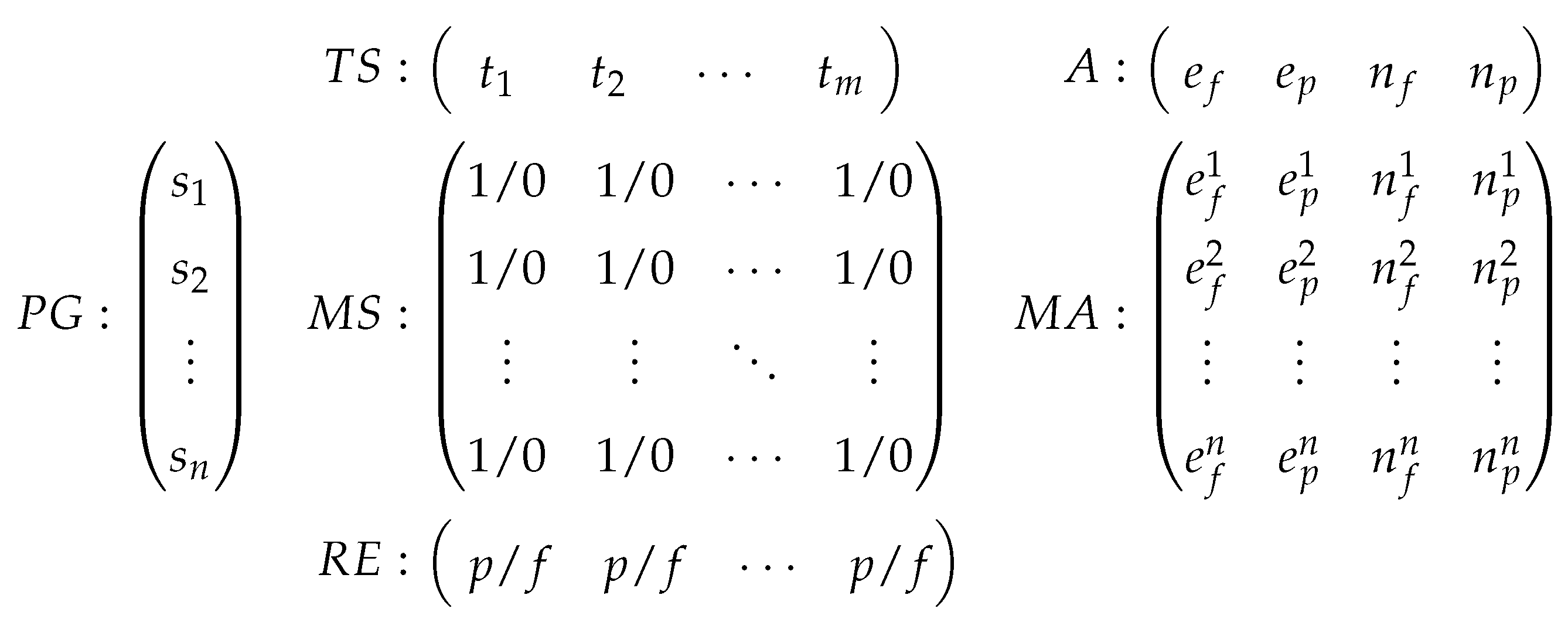
Given a program $\mathit{PG}$ with n statements ($s_1$, $s_2$, …, $s_n$) and a test suite $\mathit{TS}$ with m test cases ($t_1$, $t_2$, …, $t_m$), Figure 1 depicts the relationships among all the essential information for SBFL [14]. The $n\times m$ matrix $\mathit{MS}$ records the coverage information for each statement in $\mathit{PG}$ with respect to each test case in $\mathit{TS}$. If statement $s_i$ is executed by test case $t_j$, the entry in the i-th row and j-th column of $\mathit{MS}$ will be marked as “1”. Otherwise, it will be marked as “0”. The $1\times m$ matrix $\mathit{RE}$ represents the testing result of individual test case in terms of pass (p) or fail (f). The $1\times 4$ matrix $\mathit{A}$ represents four important quantities for each statement in the program. These four quantities are (1) the number of test cases that execute the statement and fail the program, denoted as $e_f$; (2) the number of test cases that execute the statement and pass the program, denoted as $e_p$; (3) the number of test cases that do not execute the statement and fail the program, denoted as $n_f$; and (4) the number of test cases that do not execute the statement and pass the program, denoted as $n_p$. Obviously, the sum of these four quantities is equal to the size of the test suite $\mathit{TS}$; that is $e_f+e_p+n_f+n_p=m$ [14]. The sum of $e_f$ and $n_f$ is equal to the total number of failed test cases, denoted by F, and the sum of $e_p$ and $n_p$ is equal to the total number of passed test cases, denoted by P. That is, $e_f+n_f=F$, $e_p+n_p=P$. Also, $0⩽e_f,n_f⩽F$ and $0⩽e_p,n_p⩽P$. Finally, the $n\times 4$ matrix $\mathit{MA}$ summarizes these quantities for all statements in program $\mathit{PG}$, which will be used to calculate the risk values according to different risk evaluation formulas.

2.2. Risk Evaluation Formulas

After constructing the program spectrum information, a risk evaluation formula is designed to compute a risk value which is used to indicate the likelihood of a program entity being faulty. The program entity that has a greater risk value will have a higher chance of being faulty. Many classical formulas have been proposed and widely used, such as Tarantula [23], Jaccard [24], Ochiai [7], Wong formulas [9,25,26], Naish formulas [13], and genetic programming (GP) formulas [14,27]. The program entity used in these formulas are at the statement level. The program statement with greater risk value is more likely to contain fault. Debuggers then rank the program statements in descending order of their risk values. As a result, debuggers should inspect those program statements appearing on the top of the ranking list. Therefore, it is fundamental to choose the most effective formula to make faulty statements rank as high as possible.

In order to analyze the effectiveness of various formulas, both empirical and theoretical studies have been conducted by many researchers. However, the empirical analysis strongly depends on the experimental setup, in which subject programs, fault types, and the size of test suite are the most effective threats to experimental results. Therefore, to solve the inaccuracy problem in empirical study, some theoretical analysis are proposed to investigate the performance of risk evaluation formulas.

In [11,14,15], the investigation is on comparing two risk evaluation formulas and identifying maximal risk evaluation formula in a group of risk evaluation formulas. Please be reminded that the risk evaluation formula is used by the debugger to generate a ranking list of program spectra. If a formula can “put” the faulty spectrum in a higher position in the ranking list than that of another formula, the former formula is said to perform better than the latter formula. In the first aspect, the study of Xie et al. [14] divides program statements in the program under test into three mutually exclusive subsets: the subset that contains all statements with risk values greater than (denoted as $S_B^R$), equal to (denoted as $S_F^R$), and smaller than (denoted as $S_A^R$) that of the faulty statement in the program, assuming the program only contains one faulty statement where R is the risk evaluation formula. Please note that the faulty statement must be in $S_F^R$ because it contains all statements that have the same risk value as the faulty statement. Loosely speaking, these three subsets divide the ranking list into three parts: the top part being $S_B^R$ because its statements appear “before” the faulty statement, since its risk values are greater than that of the faulty statement; the middle part being $S_F^R$; and the bottom part being $S_A^R$ because it appears “after” the faulty statement. Given any two formulas $R_1$ and $R_2$, a program with a faulty statement and a test suite, $R_1$ is said to be equivalent to $R_2$ (denoted by $R_1\leftrightarrow R_2$) when $S_B^{R_1}=S_B^{R_2}$, $S_F^{R_1}=S_F^{R_2}$ and $S_A^{R_1}=S_A^{R_2}$. While in [12,13], two equivalent risk evaluation formulas require strictly identical ranking lists. Furthermore, $R_1$ is said to be better than $R_2$ (denoted by $R_1\to R_2$) if $S_B^{R_1}\subseteq S_B^{R_2}$ and $S_A^{R_2}\subseteq S_A^{R_1}$. This is because $R_1$ will place the faulty statement earlier in the ranking list than $R_2$. As a result, debugger using the ranking list from $R_1$ will get to reach the faulty statement earlier than using $R_2$. As can be seen from the definition of “better”, the set of all risk evaluation formulas equipped with the “better” relation becomes a partially ordered set (poset). As a result, the maximal elements in this poset will then be referred to as “maximal risk evaluation formulas” or simply “maximal formulas”, if it is clear from the context. Following the definition in [14], a formula $R_1$ is said to be a maximal formula in a set S of formulas, if for any formula $R_2\in S$, $R_2$ is better than $R_1$ implies $R_2$ is equivalent to $R_1$ because no other formulas can outperform a maximal formula.

The theoretical analysis in [11,14,15] shows that among 30 risk evaluation formulas, there are five maximal formulas with the assumption that only one fault is in the program. Moreover, these five formulas can be grouped into two groups in which all formulas in the same group have the same performance. These two maximal groups are $ER1$ and ${\mathit{ER}}_5$. Formulas in $ER1$ are Naish1 (abbreviated as N1) and Naish2, both are from [13], whereas formulas in ${\mathit{ER}}_5$ are Wong1 (abbreviated as W1) from [9], Russel & Rao from [28], and Binary from [13]. In the follow-up work [16,17], the researchers proposed to use genetic programming (GP) techniques to come up with 30 GP-evolved risk evaluation formulas. Among these 30 GP-evolved formulas, they further identified four more maximal formulas; namely, GP02, GP03, GP13, and GP19 [27]. Moreover, GP13 was proven to be equivalent to those maximal formulas in the $ER1$ group [16]. As a result, the $ER1$ group is now denoted as ${\mathit{ER}}_1^{{}^{\prime }}$, which also includes GP13. The other three GP-evolved formulas form three new groups of maximal formulas. In summary, among 60 risk evaluation formulas, there are nine maximal formulas which can be grouped into five maximal formula groups. All five maximal formula groups are listed in

Table 1. Maximal risk evaluation formula groups.

Group	Risk Evaluation Formula	Expression
${\mathit{ER}}_1^{{}^{\prime }}$	Naish1 (abbr. N1)	$\left\{\begin{array}{cc}-1\hfill & \mathrm{if}{e}_f<F\hfill \\ n_p\hfill & \mathrm{if}{e}_f=F\hfill \end{array}\right.$
	Naish2	$e_f-\frac{e_p}{e_p+n_p+1}$
	GP13	$e_f(1+\frac{1}{2e_p+e_f})$
${\mathit{ER}}_5$	Wong1 (abbr. W1)	$e_f$
	Russel & Rao	$\frac{e_f}{e_f+n_f+e_p+n_p}$
	Binary	$\left\{\begin{array}{cc}0\hfill & \mathrm{if}{e}_f<F\hfill \\ 1\hfill & \mathrm{if}{e}_f=F\hfill \end{array}\right.$
GP02		$2(e_f+\sqrt{n_p})+\sqrt{e_p}$
GP03		$\sqrt{|e_f^2-\sqrt{e_p}|}$
GP19		$e_f\sqrt{|e_p-e_f+n_f-n_p|}$

.

Since no other formulas can outperform the formulas in these five maximal risk evaluation formula groups, it is intuitively appealing to do more research work on comparing the performance across these five maximal formula groups. Furthermore, Yoo et al. [18] showed that there never exists a greatest formula outperforming all other formulas.

3. A Condition with Which to Compare Risk Evaluation Formulas

3.1. Comparing Two Risk Evaluation Formulas

In this section, we propose a new approach to compare between two risk evaluation formulas. Let us discuss the approach used to judge whether a risk evaluation formula is better than another in previous work.

As mentioned previously, given a risk evaluation formula R, the ranking list can be divided into three mutually exclusive subsets, $S_B^R$, $S_F^R$, and $S_A^R$, in which statements are ranked with their suspiciousness. Empirical or theoretical comparison of two risk evaluation formulas $R_1$ and $R_2$ is then judged by the possible situations arising from six subsets: $S_B^{R_1}$, $S_F^{R_1}$, $S_A^{R_1}$, $S_B^{R_2}$, $S_F^{R_2}$, and $S_A^{R_2}$. For empirical study, researchers use the exact locations of the faulty statement appearing in the ranking lists of $R_1$ and $R_2$ to compare. So, the faulty statement will be in $S_F^{R_1}$ and in $S_F^{R_2}$. For $R_1$ to be better than $R_2$, the exact location of the faulty statement in $R_1$’s ranking list should be higher than that in $R_2$.

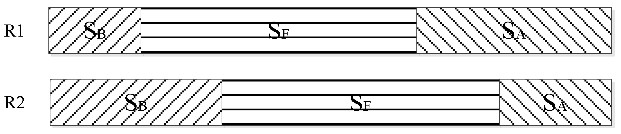
On the other hand, for theoretical comparison of two risk evaluation formulas $R_1$ and $R_2$, $R_1$ is said to perform better than $R_2$ if “$S_B^{R_1}\subseteq S_B^{R_2}$ and $S_A^{R_1}\supseteq S_A^{R_2}$” [14]. Figure 2 depicts this situation. In fact, when $S_B^{R_1}=S_B^{R_2}$ and $S_A^{R_1}=S_A^{R_2}$, $R_1$ and $R_2$ have the same performance. In addition, readers may argue the fact that this may not be very accurate. For example, after the ranking, if the “actual faulty statement” is located at the end of $S_F^{R_1}$ for $R_1$ and is located in the front of $S_F^{R_2}$ for $R_2$, $R_2$ can perform better than $R_1$. The concept of consistent tie-breaking scheme is assumed in the theoretical study. This assumption of using consistent tie-breaking to compare the performance between two formulas seems reasonable without further information.

Based on this idea, we propose a new condition for comparing two risk evaluation formulas $R_1$ and $R_2$. We first define our notations. For a risk evaluation formula R, we use $n_B^R$, $n_F^R$ and $n_A^R$ to denote the number of statements in $S_B^R$, $S_F^R$, and $S_A^R$. Let n denote the total number of statements in a program. Please observe that $n=n_B^R+n_F^R+n_A^R$. We now define the expected faulty location, EFL, of a risk evaluation formula R by

$$EFL(R)=n_B^R+\frac{1}{2}{n}_F^R$$

(1)

where $n_B^R$ and $n_F^R$ are the numbers of statements in $S_B^R$ and $S_F^R$ respectively. This is, in fact, the expected location of the faulty statement in the ranking list generated by the risk evaluation formula R. Please observe that $EFL(R)=n_B^R+\frac{1}{2}{n}_F^R=n_B^R+\frac{1}{2}(n-n_B^R-n_A^R)=\frac{1}{2}(n+n_B^R-n_A^R)$. By assuming that the faulty statement is at the middle of $S_F^R$, we can then calculate the ranking of the faulty statement.

We now formally define our condition for comparing two risk evaluation formulas. For two risk evaluation formulas $R_1$ and $R_2$, we said that $R_1$ performs better than $R_2$ if the expected faulty location of $R_1$ is in front of that of $R_2$; that is, $EFL(R_1)<EFL(R_2)$. We have the following proposition.

Proposition 1.

For any two risk evaluation formulas $R_1$ and $R_2$, if $n_B^{R_1}-n_A^{R_1}<n_B^{R_2}-n_A^{R_2}$, then $R_1$ performs better than $R_2$.

Proof. 

For any two risk evaluation formulas $R_1$ and $R_2$, the expected faulty locations of $R_1$ and $R_2$ are $EFL(R_1)=\frac{1}{2}(n+n_B^{R_1}-n_A^{R_1})$ and $EFL(R_2)=\frac{1}{2}(n+n_B^{R_2}-n_A^{R_2})$ respectively. Since $n_B^{R_1}-n_A^{R_1}<n_B^{R_2}-n_A^{R_2}$, the expected faulty location for $R_1$ is in front of that for $R_2$; that is, $EFL(R_1)<EFL(R_2)$. Hence, $R_1$ performs better than $R_2$. □

3.2. Five Scenarios for One Formula Better Than Another

In a previous study [14], formula $R_1$ is said to be better than $R_2$ with the condition “$S_B^{R_1}\subseteq S_B^{R_2}$ and $S_A^{R_1}\supseteq S_A^{R_2}$”, which means that the number of statements in $S_B^{R_1}$ is smaller than that in $S_B^{R_2}$, and the number of statements in $S_A^{R_1}$ is larger than that in $S_A^{R_2}$. However, our experimental results show that this is not the only scenario for one formula better than another. In the following, we present five scenarios when a risk evaluation formula $R_1$ performs better than $R_2$. We denote them as $B_{(<)}{A}_{(>)}$, $B_{(<)}{A}_{(=)}$, $B_{(<)}{A}_{(<)}$, $B_{(=)}{A}_{(>)}$, and $B_{(>)}{A}_{(>)}$, where (1) B indicates the comparison pair between the number of statements in the subsets $S_B^{R_1}$ and $S_B^{R_2}$; (2) A represents the comparison pair between the number of statements in the subsets $S_A^{R_1}$ and $S_A^{R_2}$; and (3) <, =, and > respectively mean the former number is smaller than, equal to, and larger than the latter one. They are

• $B_{(<)}{A}_{(>)}$: When $n_B^{R_1}<n_B^{R_2}$ and $n_A^{R_1}>n_A^{R_2}$, we have $n_B^{R_1}-n_A^{R_1}<n_B^{R_2}-n_A^{R_1}<n_B^{R_2}-n_A^{R_2}$.
• $B_{(<)}{A}_{(=)}$: When $n_B^{R_1}<n_B^{R_2}$ and $n_A^{R_1}=n_A^{R_2}$, we have $n_B^{R_1}-n_A^{R_1}<n_B^{R_2}-n_A^{R_1}=n_B^{R_2}-n_A^{R_2}$.
• $B_{(<)}{A}_{(<)}$: When $n_B^{R_1}<n_B^{R_2}$, $n_A^{R_1}<n_A^{R_2}$ and $n_B^{R_1}-n_A^{R_1}<n_B^{R_2}-n_A^{R_2}$, it is obvious that $n_B^{R_1}-n_A^{R_1}<n_B^{R_2}-n_A^{R_2}$.
• $B_{(=)}{A}_{(>)}$: When $n_B^{R_1}=n_B^{R_2}$ and $n_A^{R_1}>n_A^{R_2}$, we have $n_B^{R_1}-n_A^{R_1}=n_B^{R_2}-n_A^{R_1}<n_B^{R_2}-n_A^{R_2}$.
• $B_{(>)}{A}_{(>)}$: When $n_B^{R_1}>n_B^{R_2}$, $n_A^{R_1}>n_A^{R_2}$ and $n_B^{R_1}-n_A^{R_1}<n_B^{R_2}-n_A^{R_2}$, it is obvious that $n_B^{R_1}-n_A^{R_1}<n_B^{R_2}-n_A^{R_2}$.

Figure 3 depicts these five different scenarios, which cover all possible cases when one risk evaluation formula performs better than another one.

4. Empirical Study

4.1. Subject Programs and Test Suite

Eleven C programs whose number of executable statements (eLOC) range from 135 to 9932 with an average of 3137.8 eLOC were selected for our study. The eLOCs of these programs were counted by SLOCCount 2.26 [29]. These programs were selected because they have been used in fault localization experiments performed by other researchers [25,30,31,32]. These programs were downloaded from the Software-artifact Infrastructure Repository (SIR) [33]. These 11 programs are (1) three UNIX utilities, namely, flex, grep, and sed; (2) one real life application space; and (3) seven small programs usually referred to as the Siemens suite. The following is a description of these 11 programs.

• Flex is an UNIX utility to generate lexical analyzer by scanning a lex file with definitions, rules, and user code contained. The generated analyzer then transforms the input stream into a sequence of tokens.
• Grep is a pattern matching engine. Given one or more patterns and some input files for searching, it outputs the lines that match one or more of the patterns.
• Sed is a stream editor to perform operations on the input stream, such as replacement, deletion, and insertion on a specific line or the global text.
• Space is an interpreter for an array definition language (ADL) to check the ADL grammar and specific consistency rules. If the ADL file is correct, space outputs an array data file; otherwise, the program outputs error messages.
• Print_tokens and print_tokens2 are two lexical parsers used to group input strings into tokens and identify the token categories. The main difference between these two programs is that print_tokens uses a hard-coded DFA, while print_tokens2 does not.
• Replace is a program of regular expression matching and substitution. It replaces any substring matched by the input regular expression with a replacement string, and outputs a new file.
• Schedule and schedule2 are used to schedule the priority in three job lists. Schedule is non-preemptive and schedule2 is preemptive.
• Tcas is used to avoid air accident by detecting on-board conflict through radar system and providing a resolution advice, such as climb, descend, or remain on the current trajectory.
• Tot_info takes a set of tables as input and outputs the Kullbacks information measure, degrees of freedom, and possibility density of a ${\chi }^2$ distribution for each table and the summary of the entire set.

Since previous fault localization investigations on the effectiveness of risk evaluation formulas have the assumption that the faulty program contains one fault, e.g., [14], we used the same assumption in our empirical study. Related to the faulty versions of these 11 programs on SIR, some of them have multiple faults, and hence, were excluded from our experiments. For the three UNIX utilities, it is unfortunate that all their faulty versions contain multiple faults. Hence, we manually generated five faulty versions for each of these UNIX utilities and each faulty version contained only one single fault. The space program has 38 faulty versions with real faults. Only seven out of these 38 faulty versions contain single faults, and hence were selected for our experiments. The Siemens suite includes seven small C programs with various seeded faults in their faulty versions. Some of these faulty versions were excluded from our experiments as they contain more than one fault. Most of the faulty statements are conditional statements and assignment statements. For example, the faulty statement of print_tokens2 v6 is “if (isdigit(*(str+i+1)))”, which should be “if (isdigit(*(str+i)))”. A faulty version that is selected or manually generated for our empirical study is referred to as a “selected faulty version” whenever it is clear from the context.

Table 2. Subject programs and test suite.

Program	eLOC	Faulty Versions Selected for Empirical Study	(Number/Total)	Test Suite Size	Description
flex 1.1	9932	m1, m2, m3, m4, m5	(5 / 5)	670	lexical scanner
grep 1.2	7306	m1, m2, m3, m4, m5	(5 / 5)	806	pattern match
sed 2.0	9205	m1, m2, m3, m4, m5	(5 / 7)	441	stream editor
Space 2.0	5902	v14, v15, v18, v20, v23, v26, v33	(7 / 38)	13,550	ADL interpreter
print_tokens 2.0	342	v5, v7	(2 / 7)	4130	lexical analyzer
print_tokens2 2.0	355	v4, v5, v6, v7, v8, v9, v10	(7 / 10)	4115	lexical analyzer
replace 2.1	512	v1, v15, v30	(3 / 32)	5542	pattern match
schedule 2.0	292	v3, v4	(2 / 9)	2650	priority scheduler
schedule2 2.0	262	v6, v7, v10	(3 / 10)	2710	priority scheduler
tcas 2.0	135	v1	(1 / 41)	1608	altitude separation
tot_info 2.0	273	v5, v7, v8, v15, v16, v17, v20, v23	(8 / 23)	1052	information measure

summarizes the information of these programs for our empirical study. As discussed earlier, the eLOC column reports the number of executable statements collected by SLOCCount 2.26 [29]. The mutants generated from the UNIX utilities, the selected faulty versions of space and the Siemens suite, the number of manually mutated or selected faulty versions, and the total number of faulty versions provided in SIR are listed in the third column. The size of each test suite is listed in the second to last column—obtained from the individual “universe” test plan. In summary, our empirical study had 15 mutants for the three UNIX utilities, seven faulty versions for the space program, and 26 faulty versions for the Siemens suite. The size of the corresponding test suite ranged from 441 to 13,550 test cases, with an average of 3782.9 test cases per selected faulty version.

4.2. The Empirical Process

We performed an empirical study to compare the effectiveness of five maximal formula groups, ${\mathit{ER}}_1^{{}^{\prime }}$, ${\mathit{ER}}_5$, GP02, GP03 and GP19. It has been proven by Xie et al. [14] that all formulas in the same maximal formula group have the same performance. Therefore, it is sufficient to select only one representative formula from each group for study. In other words, if another formula is chosen, we would still observe the same results. We chose Naish1 (abbreviated as N1) from ${\mathit{ER}}_1^{{}^{\prime }}$ and Wong1 (abbreviated as W1) from ${\mathit{ER}}_5$ because they are the simplest formulas in their own groups. We chose GP02, GP03, and GP19 from the last three groups because there is only one maximal formula contained in each group.

The empirical study aimed to compare the performance of these formulas in a pairwise manner. As a result, we have 10 comparison pairs. For ease of reference, we use CP1–CP10 to denote these 10 pairs, in which CP1 denotes the comparison pair between N1 and W1, CP2 for N1 and GP02, CP3 for N1 and GP03, CP4 for N1 and GP19, CP5 for W1 and GP02, CP6 for W1 and GP03, CP7 for W1 and GP19, CP8 for GP02 and GP03, CP9 for GP02 and GP19, and finally, CP10 for GP03 and GP19.

For the selected 11 C programs, there were, altogether, 48 faulty versions selected for the empirical study. For each selected faulty version, it was executed with respect to its corresponding test suite. All of the executions of faulty programs with respect to their test suites were performed using Fedora 20 64-bit virtual machine with one processor and 4GB of memory. After the execution, all information related to the program spectrum was recorded; namely, $e_f^i$, $e_p^i$, $n_f^i$, and $n_p^i$, for every statement $s_i$ in the selected faulty version. Once all information had been collected, we then applied the five maximal risk evaluation formulas, each from its own formula group, to calculate the risk values for each statement and get the corresponding ranking lists. As a reminder, statements with the same risk value were then ordered according to their corresponding statement IDs in the faulty program. For each maximal formula R in {N1, W1, GP02, GP03, and GP19}, we then divided its ranking list into three mutually exclusive subsets; namely, $S_B^R$, $S_F^R$, and $S_A^R$. We then calculated the expected faulty location, $EFL$, of the risk evaluation formula R using the formula $EFL(R)=n_B^R+\frac{1}{2}{n}_F^R$.

Once we calculated all the expected faulty locations of these five formulas, we performed our analysis on the pairwise comparison between these formulas. For each comparison pair of formulas $R_1$ and $R_2$, we conclude that $R_1$ performs better than $R_2$ on that instance of the selected faulty version when $EFL(R_1)<EFL(R_2)$. When $EFL(R_1)=EFL(R_2)$, the two formulas have the same performance. When $EFL(R_2)<EFL(R_1)$, we conclude that $R_2$ performs better than $R_1$.

4.3. Experimental Results and Analysis

Table 3. Performances of various comparisons of the five maximal formulas.

Subject Program	CP1	CP2	CP3	CP4	CP5	CP6	CP7	CP8	CP9	CP10
	N1,W1	N1,GP02	N1,GP03	N1,GP19	W1,GP02	W1,GP03	W1,GP19	GP02,GP03	GP02,GP19	GP03,GP19
flex m1	N1	N1	N1	N1	W1	W1	W1	GP02	GP02	same
flex m2	W1	N1	N1	GP19	W1	W1	GP19	GP03	GP19	GP19
flex m3	N1	GP02	N1	N1	GP02	W1	same	GP02	GP02	GP19
flex m4	N1	same	N1	N1	GP02	W1	W1	GP02	GP02	GP19
flex m5	N1	same	same	same	GP02	GP03	GP19	same	same	same
grep m1	N1	N1	N1	N1	GP02	GP03	W1	GP03	GP02	GP03
grep m2	W1	N1	same	GP19	W1	W1	GP19	GP03	GP19	GP19
grep m3	N1	N1	same	N1	W1	GP03	W1	GP03	GP19	GP03
grep m4	W1	GP02	GP03	GP19	same	same	same	same	same	same
grep m5	W1	GP02	GP03	GP19	W1	GP03	GP19	GP03	GP19	GP03
sed m1	W1	GP02	GP03	GP19	W1	W1	GP19	GP03	GP19	GP19
sed m2	N1	same	same	N1	GP02	GP03	W1	same	GP02	GP03
sed m3	N1	N1	same	N1	GP02	GP03	W1	GP03	GP02	GP03
sed m4	W1	N1	same	GP19	W1	W1	GP19	GP03	GP19	GP19
sed m5	W1	N1	same	GP19	W1	W1	GP19	GP03	GP19	GP19
space v14	N1	N1	N1	N1	W1	same	W1	GP03	GP02	GP03
space v15	N1	same	N1	N1	GP02	same	W1	GP02	GP02	GP03
space v18	N1	N1	same	N1	GP02	GP03	W1	GP03	GP02	GP03
space v20	N1	N1	GP03	N1	GP02	GP03	W1	GP03	GP02	GP03
space v23	N1	N1	N1	N1	GP02	W1	W1	GP02	GP02	GP03
space v26	W1	GP02	GP03	GP19	GP02	same	same	GP02	GP02	same
space v33	N1	N1	same	N1	GP02	GP03	W1	GP03	GP02	GP03
print_tokens v5	N1	same	same	N1	GP02	GP03	W1	same	GP02	GP03
print_tokens v7	N1	N1	same	N1	GP02	GP03	W1	GP03	GP02	GP03
print_tokens2 v4	N1	N1	same	N1	GP02	GP03	W1	GP03	GP02	GP03
print_tokens2 v5	N1	N1	same	same	GP02	GP03	GP19	GP03	GP19	same
print_tokens2 v6	N1	N1	same	same	GP02	GP03	GP19	GP03	GP19	same
print_tokens2 v7	N1	GP02	same	N1	GP02	GP03	W1	GP02	GP02	GP03
print_tokens2 v8	N1	N1	same	N1	GP02	GP03	W1	GP03	GP02	GP03
print_tokens2 v9	N1	same	same	N1	GP02	GP03	W1	same	GP02	GP03
print_tokens2 v10	N1	GP02	same	N1	GP02	GP03	W1	GP02	GP02	GP03
replace v1	N1	same	same	N1	GP02	GP03	W1	same	GP02	GP03
replace v15	W1	N1	same	GP19	W1	W1	GP19	GP03	GP19	GP19
replace v30	N1	GP02	same	N1	GP02	GP03	W1	GP02	GP02	GP03
schedule v3	N1	same	same	N1	GP02	GP03	W1	same	GP02	GP03
schedule v4	N1	same	same	N1	GP02	GP03	W1	same	GP02	GP03
schedule2 v6	N1	N1	N1	N1	W1	W1	W1	GP02	GP19	GP19
schedule2 v7	W1	N1	same	GP19	W1	W1	GP19	GP03	GP19	GP19
schedule2 v10	W1	N1	same	GP19	W1	W1	GP19	GP03	GP19	GP19
tcas v1	N1	GP02	same	N1	GP02	GP03	W1	GP02	GP02	GP03
tot_info v5	N1	N1	same	N1	W1	GP03	W1	GP03	GP02	GP03
tot_info v7	N1	same	same	N1	GP02	GP03	W1	same	GP02	GP03
tot_info v8	N1	N1	same	same	GP02	GP03	GP19	GP03	GP19	same
tot_info v15	N1	N1	same	same	GP02	GP03	GP19	GP03	GP19	same
tot_info v16	W1	same	same	GP19	W1	W1	GP19	same	GP19	GP19
tot_info v17	N1	same	same	N1	GP02	GP03	W1	same	GP02	GP03
tot_info v20	same	N1	same	same	W1	same	same	GP03	GP19	same
tot_info v23	N1	same	same	N1	GP02	GP03	W1	same	GP02	GP03

lists all the results of these 10 comparison pairs. For example, “N1” in the cell of row “tcas v1” and column “CP1” indicates that “N1 performs better than W1”. Some cells in Table 3 have “same” meaning that the two risk formulas in the comparison pair have the same performance.

Since the performance of maximal formulas in each comparison pair varies with different programs,

Table 4. Comparison results as percentages of one formula being better than another (%).

Comparison Pair		Flex	Grep	Sed	Space	print_tokens	print_tokens2	Replace	Schedule	schedule2	tcas	tot_info	Average
CP1	N1 better	80	40	40	85.7	100	100	66.7	100	33.3	100	75	74.6
	same	0	0	0	0	0	0	0	0	0	0	12.5	1.1
	W1 better	20	60	60	14.3	0	0	33.3	0	66.7	0	12.5	24.3
CP2	N1 better	40	60	60	71.4	50	57.1	33.3	0	100	0	50	47.4
	same	40	0	20	14.3	50	14.3	33.3	100	0	0	50	29.3
	GP02 better	20	40	20	14.3	0	28.6	33.3	0	0	100	0	23.3
CP3	N1 better	80	20	0	42.9	0	0	0	0	33.3	0	0	16.0
	same	20	40	80	28.6	100	100	100	100	66.7	100	100	75.9
	GP03 better	0	40	20	28.6	0	0	0	0	0	0	0	8.1
CP4	N1 better	60	40	40	85.7	100	71.4	66.7	100	33.3	100	50	67.9
	same	20	0	0	0	0	28.6	0	0	0	0	37.5	7.8
	GP19 better	20	60	60	14.3	0	0	33.3	0	66.7	0	12.5	24.3
CP5	W1 better	40	60	60	14.3	0	0	33.3	0	100	0	37.5	31.4
	same	0	20	0	0	0	0	0	0	0	0	0	1.8
	GP02 better	60	20	40	85.7	100	100	66.7	100	0	100	62.5	66.8
CP6	W1 better	80	20	60	14.3	0	0	33.3	0	100	0	12.5	29.1
	same	0	20	0	42.9	0	0	0	0	0	0	12.5	6.9
	GP03 better	20	60	40	42.9	100	100	66.7	100	0	100	75	64.0
CP7	W1 better	40	40	40	85.7	100	71.4	66.7	100	33.3	100	50	66.1
	same	20	20	0	14.3	0	0	0	0	0	0	12.5	6.1
	GP19 better	40	40	60	0	0	28.6	33.3	0	66.7	0	37.5	27.8
CP8	GP02 better	60	0	0	42.9	0	28.6	33.3	0	33.3	100	0	27.1
	same	20	20	20	0	50	14.3	33.3	100	0	0	50	28.0
	GP03 better	20	80	80	57.1	50	57.1	33.3	0	66.7	0	50	44.9
CP9	GP02 better	60	20	40	100	100	71.4	66.7	100	0	100	50	64.4
	same	20	20	0	0	0	0	0	0	0	0	0	3.6
	GP19 better	20	60	60	0	0	28.6	33.3	0	100	0	50	32.0
CP10	GP03 better	0	60	40	85.7	100	71.4	66.7	100	0	100	50	63.9
	same	40	20	0	14.3	0	28.6	0	0	0	0	37.5	10.2
	GP19 better	60	20	60	0	0	0	33.3	0	100	0	12.5	26.0

summarizes the results as the percentage of “$R_1$ which performs better than $R_2$”, “$R_1$ which performs the same as $R_2$”, and “$R_2$ which performs better than $R_1$” for each comparison pair and each individual subject program. For example, in the row of “CP1” and the column of flex, out of the five mutant programs, there are four mutants for which N1 performs better than W1 and there is only one mutant for which W1 performs better than N1. Hence, we can conclude that, among these five mutants of flex, N1 performs better than W1 more often. For ease of reference, we use the term more-frequently-better to reflect this situation. In other words, we conclude that N1 performs more-frequently-better than W1. Formally, for two risk evaluation formulas $R_1$ and $R_2$, we say that $R_1$ performs more-frequently-better than $R_2$, denoted as $R_1⤏R_2$, if, among all selected faulty versions, the number of times that “$R_1$ performs better than $R_2$” is higher than that of “$R_2$ performs better than $R_1$”.

From Table 4, we have the following observations.

(1)

N1 has a higher chance to perform better than W1, GP02, GP03, and GP19.

• For CP1, we observe that N1 has a higher chance to perform better than W1 for all programs except grep, sed, and schedule2. The percentage values of $\mathrm{N}1⤏\mathrm{W}1$ range from 33.3% to 100% with an average of 74.6%, whereas those of $\mathrm{W}1⤏\mathrm{N}1$ range from 0% to 66.7% with an average of 24.3%. Hence, we can conclude that N1 performs more-frequently-better than W1.
• Similarly, for CP2, CP3 and CP4, we can also conclude that N1 has a higher chance to perform better than GP02, GP03, and GP19, respectively. However, we have to point out an interesting observation of the N1 and GP03 pair. For N1 and GP03, the percentages of $\mathrm{N}1⤏\mathrm{GP}03$ range from 0% to 80% with an average of 16.0%, whereas those of $\mathrm{GP}03⤏\mathrm{N}1$ range from 0% to 40% with an average of 8.1%. In fact, N1 and GP03 have the same performance with an average of 75.9%.

(2)

GP03 has a higher chance to perform better than W1, GP02 and GP19.

• For CP8, GP03 has a higher chance to perform better than GP02 for all programs except flex, replace, schedule, and tcas. In fact, for replace and schedule, the chances for $\mathrm{GP}03⤏\mathrm{GP}02$ and that of $\mathrm{GP}02⤏\mathrm{GP}03$ are the same; both are 0% for schedule and 33.3% for replace. The percentage values of $\mathrm{GP}03⤏\mathrm{GP}02$ range from 0% to 80% with an average of 44.9%, whereas those of $\mathrm{GP}02⤏\mathrm{GP}03$ range from 0% to 100% with an average of 27.1%. Hence, we can conclude that GP03 performs more-frequently-better than GP02.
• Similarly, for CP6 and CP10, we can also conclude that GP03 performs more-frequently-better than W1 and GP19 since the average percentage values of $\mathrm{GP}03⤏\mathrm{W}1$ and $\mathrm{GP}03⤏\mathrm{GP}19$ are 64.0% and 63.9% respectively.

(3)

GP02 has a higher chance to perform better than W1 and GP19.

• For CP5, we observe that GP02 performs more-frequently-better than W1 for all programs except grep, sed and schedule2. The percentage values of $\mathrm{GP}02⤏\mathrm{W}1$ range from 0% to 100% with an average of 66.8% whereas those of $\mathrm{W}1⤏\mathrm{GP}02$ range from 0% to 100% with an average of 31.4%. Hence, we can conclude that GP02 performs more-frequently-better than W1.
• Similarly, for CP9, we can also conclude that GP02 performs more-frequently-better than GP19.

(4)

W1 has a higher chance to perform better than GP19.

• For CP7, W1 performs more-frequently-better than GP19 for all programs except flex, grep, sed and schedule2. In fact, for flex and grep, the chances for $\mathrm{W}1⤏\mathrm{GP}19$ and that of $\mathrm{GP}19⤏\mathrm{W}1$ are the same; both are 40% for flex and 40% for grep. The percentage values of $\mathrm{W}1⤏\mathrm{GP}19$ range from 33.3% to 100% with an average of 66.1% whereas those of $\mathrm{GP}19⤏\mathrm{W}1$ range from 0% to 66.7% with an average of 27.8%. Hence, we can conclude that W1 performs more-frequently-better than GP19.

In summary, it is very likely to observe that N1 ⤏ GP03 ⤏ GP02 ⤏ W1 ⤏ GP19.

An interested reader may argue that the result of “N1 ⤏ GP03 ⤏ GP02 ⤏ W1 ⤏ GP19” is based on the percentage of the selected faulty versions per individual program, and we compare them by taking the average of these percentages. This may be unfair because, for tcas, there is only one selected faulty version. Only tcas v1 was selected as the faulty version since the scale of tcas subject program is too small, and most of the faulty versions are of the same type. Hence, a 100% of $\mathrm{N}1⤏\mathrm{W}1$ in tcas may actually add some advantages to N1 compared with other individual programs. So, one may then ask what the result would be if we used the total number of selected faulty versions to compare between these risk evaluation formulas. The answer to this question is, “We would have the same result.” We are going to discuss this in the rest of this paragraph.

Table 5. Comparison results as number of selected faulty versions that one formula is better than another.

Comparison Pair (${\mathit{R}}_1$ vs. ${\mathit{R}}_2$)	${\mathit{R}}_1$ Better	${\mathit{R}}_2$ Better	${\mathit{R}}_1$ Same as ${\mathit{R}}_2$
CP1 (N1 vs. W1)	35	12	1
CP2 (N1 vs. GP02)	26	9	13
CP3 (N1 vs. GP03)	9	5	34
CP4 (N1 vs. GP19)	30	12	6
CP5 (W1 vs. GP02)	16	31	1
CP6 (W1 vs. GP03)	14	29	5
CP7 (W1 vs. GP19)	29	15	4
CP8 (GP02 vs. GP03)	11	25	12
CP9 (GP02 vs. GP19)	29	17	2
CP10 (GP03 vs. GP19)	27	12	9

shows, for each comparison pair $R_1$ and $R_2$, the total number of selected faulty versions that fall into the results of “$R_1$ better”, “$R_2$ better”, and “$R_1$ same as $R_2$”. For example, in the row of CP3 (the pair of N1 and GP03), there are nine selected faulty versions that fall into “$\mathrm{N}1$ better”, five in “$\mathrm{GP}03$ better”, and 34 in “N1 same as GP03”. Hence, N1 performs more-frequently-better than GP03. From Table 5, we have the following observations:

(1)

For CP1–CP4, N1 has a higher chance to perform better than W1, GP02, GP03, and GP19.

(2)

For CP8, CP6, and CP10, GP03 has a higher chance to perform better than GP02, W1, and GP19.

(3)

For CP5 and CP9, GP02 has a higher chance to perform better than W1 and GP19.

(4)

For CP7, W1 has a higher chance to perform better than GP19.

As a result, we have the same observation. That is, N1 ⤏ GP03 ⤏ GP02 ⤏ W1 ⤏ GP19.

Since N1 and W1 are representative formulas from their original maximal formula groups $E{R}_1^{{}^{\prime }}$ and $E{R}_5$ respectively, we can conclude further that any maximal formula in the $E{R}_1^{{}^{\prime }}$ group performs more-frequently-better than GP03, which in turns performs more-frequently-better than GP02, which in turns performs more-frequently-better than any maximal formula in the $E{R}_5$ group, which in turns performs more-frequently-better than GP19. That is, we have $E{R}_1^{{}^{\prime }}⤏\mathrm{GP}03⤏\mathrm{GP}02⤏E{R}_5⤏\mathrm{GP}19$. Here, we extend the meaning of “⤏” to compare between two maximal formula groups. In other words, if GpA and GpB are two maximal risk evaluation formula groups, GpA ⤏ GpB means $R_a⤏R_b$ where $R_a$ is a risk evaluation formula in GpA and $R_b$ is in GpB. Please be remindeded that all risk evaluation formulas in the same maximal formula group have the same performance.

As discussed in Section 3.2, when comparing between two risk evaluation formulas $R_1$ and $R_2$, there are five scenarios to characterize all possible cases of $R_1$ performs better than $R_2$.

Table 6. Scenarios covered by individual subject program.

Scenarios	Flex	Grep	Sed	Space	print_tokens	print_tokens2	Replace	Schedule	schedule2	tcas	tot_info	Total
$B_{(<)}{A}_{(>)}$	22	18	23	27	9	28	14	8	20	5	29	203
$B_{(<)}{A}_{(=)}$	6	2	2	3	0	2	0	0	0	0	0	15
$B_{(<)}{A}_{(<)}$	5	5	6	10	1	2	4	0	5	1	6	45
$B_{(=)}{A}_{(>)}$	6	7	6	2	5	9	4	3	0	1	12	55
$B_{(>)}{A}_{(>)}$	2	10	7	20	1	16	3	3	3	2	8	75
$R_1=R_2$	9	8	6	8	4	13	5	6	2	1	25	87
total	50	50	50	70	20	70	30	20	30	10	80	480

summarises the scenarios covered by each subject program. For example, for the case of “flex”, among totally 50 comparison results (10 comparison pairs × 5 mutants of flex), there are 22 comparison results of $R_1⤏R_2$ obtained from Scenario $B_{(<)}{A}_{(>)}$, six from Scenario $B_{(<)}{A}_{(=)}$, five from Scenario $B_{(<)}{A}_{(<)}$, six from Scenario $B_{(=)}{A}_{(>)}$, two from Scenario $B_{(>)}{A}_{(>)}$, and nine comparison results indicating $R_1=R_2$. As shown in Table 6, $51.7\%$ cases of $R_1⤏R_2$ fall in Scenario $B_{(<)}{A}_{(>)}$, $3.8\%$ in Scenario $B_{(<)}{A}_{(=)}$, $11.5\%$ in Scenario $B_{(<)}{A}_{(<)}$, $13.9\%$ in Scenario $B_{(=)}{A}_{(>)}$, and $19.1\%$ in Scenario $B_{(>)}{A}_{(>)}$. According to the observation, Scenario $B_{(<)}{A}_{(>)}$ covers the majority of cases that $R_1⤏R_2$.

4.4. Discussion

Yoo et al. [17] achieved a conclusion to some extent different from the conclusion in our experiment. Their results concluded that ${\mathit{ER}}_1^{{}^{\prime }}$ is the best performer, ${\mathit{ER}}_5$ is the worst in most cases, and the other three formula groups $\mathrm{GP}02$, $\mathrm{GP}03$, and $\mathrm{GP}19$ perform similarly, but with $\mathrm{GP}03$ being better than $\mathrm{GP}02$ and $\mathrm{GP}19$. The difference between their study and our study is probably because different metrics and experimental setups were used. Yoo et al. used the expense metric to measure the number of statements should be examined before the faulty statement is found. In this paper, we utilized the expected faulty location to measure the expected location of faulty statement in the faulty program. Additionally, Yoo et al. conducted an empirical study with five subject programs from SIR, including flex, grep, gzip, sed, and space. In our experiment, we performed the empirical study with 11 subject programs in which flex, grep, sed, and space were used as well. Nevertheless, their conclusion is slightly different to that of our study of ${\mathit{ER}}_1^{{}^{\prime }}⤏\mathrm{GP}03⤏\mathrm{GP}02⤏{\mathit{ER}}_5⤏\mathrm{GP}19$. Most importantly, Yoo et al. and ourselves both observed that ${\mathit{ER}}_1^{{}^{\prime }}$ is the best performer followed by GP03; that is, we have the same recommendation of using ${\mathit{ER}}_1^{{}^{\prime }}$.

4.5. Threats to Validity

4.5.1. Test Suite

There are two threats related to the test suite used in our empirical study. First is the size of the test suite. In our empirical study, we treated all test cases as one single test suite for fault localization purposes as in previous empirical study. This has been referred to as the “universe” plan in benchmarks. As mentioned in Naish et al. [13], the performance of a risk evaluation formula “may” be dependent on the actual number of test cases used in the test suite. Hence, readers should not over-generalize our results without further research. Second, it is related to the composition of test cases in a test suite. Intuitively speaking, different test cases may have different fault detection capabilities. Hence, the performance of the same risk evaluation formula may be different if two different test suites having the same number of test cases are used. It may be more interesting to investigate the diversity of test cases in a test suite to detect different types of faults in our future work.

4.5.2. Fault Type

In order to adapt to our experiment and localize the faulty statement, we excluded those faulty versions which deleted or inserted some statements in the original programs. Also, we performed our experiments on those programs with single faults. For future work, we can extend our experimental study using programs with multiple faults.

5. Related Work

The effectiveness of different SBFL techniques strongly depends on the input test suite and corresponding execution results. In contrast to the assumption of the existence of test oracles in conventional SBFL techniques, Xie et al. [34,35] presented an alleviation approach to solve the test oracle problem by using the metamorphic slice and Zhang et al. [31] used the unlabelled test cases. Additionally, a kind of test case prioritization technique is presented to improve the effectiveness of fault localization process and reduce the testing cost [36,37,38]. The FLINT has been proven to outperform similar localization techniques in 52% of the cases in [39]. Yu et al. [40] investigated different test suite reduction strategies as well for SBFL effectiveness increase.

More empirical comparisons of the performance between various formulas were also reported in [10,17]. Pearson et al. [10] compared the performances of seven different formulas on artificial faults and real faults from Defects4J and indicated that the artificial faults were not as useful as the real faults to predicate the best formula. Xu et al. [32] found that labeling perturbations influenced the robustness of risk evaluation formulas significantly, especially the impacts of mislabeling passed cases as failed cases.

6. Conclusions and Future Work

Various empirical and theoretical research works on SBFL risk evaluation formulas have been proposed to compare the performance between different formulas. Five maximal formula groups—${\mathit{ER}}_1^{{}^{\prime }}$, ${\mathit{ER}}_5$, GP02, GP03 and GP19—have been proven and it was also proven that there does not exist a greatest risk evaluation formula in terms of fault localization effectiveness. From the experimental observation, we notice that some maximal formulas can perform better than others more frequently. Hence, we propose a notion of “more-frequently-better” to compare between two maximal formulas $R_1$ and $R_2$ in this paper.

To verify our proposition that there exists one maximal formula performs more-frequently-better than another one, an empirical study on 11 C programs with real and seeded faults has been conducted. According to the experimental results, we conclude that ${\mathit{ER}}_1^{{}^{\prime }}⤏\mathrm{GP}03⤏\mathrm{GP}02⤏{\mathit{ER}}_5⤏\mathrm{GP}19$. This means, ${\mathit{ER}}_1^{{}^{\prime }}$ performs more-frequently-better than any of the other four. Therefore, we have provided a way to compare the performance between any two maximal formulas using the notion of more-frequently-better, and illustrated the feasibility of our approach with an empirical study.

Since we make the assumption that there is a single fault in the faulty program, more experimental studies using programs with multiple faults should be conducted to investigate the effectiveness of our approach.

References

- Harrold, M.J.; Rothermel, G.; Wu, R.; Yi, L. An empirical investigation of program spectra. In Acm Sigplan Notices; ACM: New York, NY, USA, 1998; Volume 33, pp. 83–90. [Google Scholar]
- Jones, J.A.; Harrold, M.J. Empirical evaluation of the tarantula automatic fault-localization technique. In Proceedings of the 20th IEEE/ACM international Conference on Automated Software Engineering, Long Beach, CA, USA, 7–11 November 2005; pp. 273–282. [Google Scholar]
- Wong, W.E.; Gao, R.; Li, Y.; Abreu, R.; Wotawa, F. A survey on software fault localization. IEEE Trans. Softw. Eng. 2016, 42, 707–740. [Google Scholar] [CrossRef] [Green Version]
- Abreu, R.; Zoeteweij, P.; Van Gemund, A.J. On the accuracy of spectrum-based fault localization. In Proceedings of the Testing: Academic and Industrial Conference Practice and Research Techniques- MUTATION (TAICPART-MUTATION 2007), Windsor, UK, 10–14 September 2007; pp. 89–98. [Google Scholar]
- Chen, Y.; Probert, R.L.; Sims, D.P. Specification-based regression test selection with risk analysis. In Proceedings of the 2002 Conference of the Centre for Advanced Studies on Collaborative Research, Toronto, ON, Canada, 30 September–3 October 2002; p. 1. [Google Scholar]
- Jones, J.A.; Harrold, M.J.; Stasko, J.T. Visualization for fault localization. In Proceedings of the ICSE 2001 Workshop on Software Visualization, Toronto, ON, Canada, 13–14 May 2001. [Google Scholar]
- Abreu, R.; Zoeteweij, P.; Van Gemund, A.J. An evaluation of similarity coefficients for software fault localization. In Proceedings of the 2006 12th Pacific Rim International Symposium on Dependable Computing (PRDC’06), Riverside, CA, USA, 18–20 December 2006; pp. 39–46. [Google Scholar]
- Abreu, R.; Zoeteweij, P.; Golsteijn, R.; Van Gemund, A.J. A practical evaluation of spectrum-based fault localization. J. Syst. Softw. 2009, 82, 1780–1792. [Google Scholar] [CrossRef]
- Wong, W.E.; Qi, Y.; Zhao, L.; Cai, K.Y. Effective fault localization using code coverage. In Proceedings of the 31st Annual International Computer Software and Applications Conference (COMPSAC 2007), Beijing, China, 24–27 July 2007; Volume 1, pp. 449–456. [Google Scholar]
- Pearson, S.; Campos, J.; Just, R.; Fraser, G.; Abreu, R.; Ernst, M.D.; Pang, D.; Keller, B. Evaluating and improving fault localization. In Proceedings of the 39th International Conference on Software Engineering, Buenos Aires, Argentina, 20–28 May 2017; pp. 609–620. [Google Scholar]
- Xie, X. On the Analysis of Spectrum-Based Fault Localization. Ph.D. Thesis, Swinburne University of Technology, Melbourne, Australia, 2012. [Google Scholar]
- Lee, H.J.; Naish, L.; Ramamohanarao, K. Study of the relationship of bug consistency with respect to performance of spectra metrics. In Proceedings of the 2009 2nd IEEE International Conference on Computer Science and Information Technology, Beijing, China, 8–11 August 2009; pp. 501–508. [Google Scholar]
- Naish, L.; Lee, H.J.; Ramamohanarao, K. A model for spectra-based software diagnosis. ACM Trans. Softw. Eng. Methodol. (TOSEM) 2011, 20, 11. [Google Scholar] [CrossRef]
- Xie, X.; Chen, T.Y.; Kuo, F.C.; Xu, B. A theoretical analysis of the risk evaluation formulas for spectrum-based fault localization. ACM Trans. Softw. Eng. Methodol. (TOSEM) 2013, 22, 31. [Google Scholar] [CrossRef]
- Chen, T.Y.; Xie, X.; Kuo, F.C.; Xu, B. A revisit of a theoretical analysis on spectrum-based fault localization. In Proceedings of the 2015 IEEE 39th Annual Computer Software and Applications Conference, Taichung, Taiwan, 1–5 July 2015; Volume 1, pp. 17–22. [Google Scholar]
- Xie, X.; Kuo, F.C.; Chen, T.Y.; Yoo, S.; Harman, M. Provably optimal and human-competitive results in sbse for spectrum based fault localisation. In International Symposium on Search Based Software Engineering; Springer: Berlin, Germany, 2013; pp. 224–238. [Google Scholar]
- Yoo, S.; Xie, X.; Kuo, F.C.; Chen, T.Y.; Harman, M. Human competitiveness of genetic programming in spectrum-based fault localisation: Theoretical and empirical analysis. ACM Trans. Softw. Eng. Methodol. (TOSEM) 2017, 26, 4. [Google Scholar] [CrossRef]
- Yoo, S.; Xie, X.; Kuo, F.C.; Chen, T.Y.; Harman, M. No pot of gold at the end of program spectrum rainbow: Greatest risk evaluation formula does not exist. RN 2014, 14, 14. [Google Scholar]
- Wong, W.E.; Sugeta, T.; Qi, Y.; Maldonado, J.C. Smart debugging software architectural design in SDL. J. Syst. Softw. 2005, 76, 15–28. [Google Scholar] [CrossRef]
- Harrold, M.J.; Rothermel, G.; Sayre, K.; Wu, R.; Yi, L. An empirical investigation of the relationship between spectra differences and regression faults. Softw. Test. Verif. Reliab. 2000, 10, 171–194. [Google Scholar] [CrossRef] [Green Version]
- Agrawal, H.; Horgan, J.R.; London, S.; Wong, W.E. Fault localization using execution slices and dataflow tests. In Proceedings of the Sixth International Symposium on Software Reliability Engineering, ISSRE’95, Toulouse, France, 24–27 October 1995; pp. 143–151. [Google Scholar]
- Wong, W.E.; Qi, Y. Effective program debugging based on execution slices and inter-block data dependency. J. Syst. Softw. 2006, 79, 891–903. [Google Scholar] [CrossRef]
- Jones, J.A.; Harrold, M.J.; Stasko, J. Visualization of test information to assist fault localization. In Proceedings of the 24th International Conference on Software Engineering, ICSE 2002, Orlando, FL, USA, 25 May 2002; pp. 467–477. [Google Scholar]
- Chen, M.Y.; Kiciman, E.; Fratkin, E.; Fox, A.; Brewer, E. Pinpoint: Problem determination in large, dynamic internet services. In Proceedings of the International Conference on Dependable Systems and Networks, Washington, DC, USA, 23–26 June 2002; pp. 595–604. [Google Scholar]
- Wong, W.E.; Debroy, V.; Choi, B. A family of code coverage-based heuristics for effective fault localization. J. Syst. Softw. 2010, 83, 188–208. [Google Scholar] [CrossRef]
- Wong, E.; Wei, T.; Qi, Y.; Zhao, L. A crosstab-based statistical method for effective fault localization. In Proceedings of the 2008 1st International Conference on Software Testing, Verification, and Validation, Lillehammer, Norway, 9–11 April 2008; pp. 42–51. [Google Scholar]
- Yoo, S. Evolving human competitive spectra-based fault localisation techniques. In International Symposium on Search Based Software Engineering; Springer: Berlin, Germany, 2012; pp. 244–258. [Google Scholar]
- Russell, P.F.; Rao, T.R. On habitat and association of species of anopheline larvae in south-eastern Madras. J. Malar. Inst. India 1940, 3, 153–178. [Google Scholar]
- SLOCCOUNT. Available online: http://www.dwheeler.com/sloccount/sloccount.html (accessed on 15 April 2019).
- Mao, X.; Lei, Y.; Dai, Z.; Qi, Y.; Wang, C. Slice-based statistical fault localization. J. Syst. Softw. 2014, 89, 51–62. [Google Scholar] [CrossRef]
- Zhang, X.Y.; Zheng, Z.; Cai, K.Y. Exploring the usefulness of unlabelled test cases in software fault localization. J. Syst. Softw. 2018, 136, 278–290. [Google Scholar] [CrossRef]
- Xu, Y.; Yin, B.; Zheng, Z.; Zhang, X.; Li, C.; Yang, S. Robustness of spectrum-based fault localisation in environments with labelling perturbations. J. Syst. Softw. 2019, 147, 172–214. [Google Scholar] [CrossRef]
- SIR. Available online: https://sir.csc.ncsu.edu/portal/index.ph (accessed on 15 April 2019).
- Xie, X.; Wong, W.E.; Chen, T.Y.; Xu, B. Spectrum-based fault localization: Testing oracles are no longer mandatory. In Proceedings of the 2011 11th International Conference on Quality Software, Madrid, Spain, 13–14 July 2011; pp. 1–10. [Google Scholar]
- Xie, X.; Wong, W.E.; Chen, T.Y.; Xu, B. Metamorphic slice: An application in spectrum-based fault localization. Inf. Softw. Technol. 2013, 55, 866–879. [Google Scholar] [CrossRef]
- Jiang, B.; Zhang, Z.; Tse, T.; Chen, T.Y. How well do test case prioritization techniques support statistical fault localization. In Proceedings of the 2009 33rd Annual IEEE International Computer Software and Applications Conference, Seattle, WA, USA, 20–24 July 2009; Volume 1, pp. 99–106. [Google Scholar]
- Jiang, B.; Chan, W. On the integration of test adequacy, test case prioritization, and statistical fault localization. In Proceedings of the 2010 10th International Conference on Quality Software, Zhangjiajie, China, 14–15 July 2010; pp. 377–384. [Google Scholar]
- Jiang, B.; Chan, W.; Tse, T. On practical adequate test suites for integrated test case prioritization and fault localization. In Proceedings of the 2011 11th International Conference on Quality Software, Madrid, Spain, 13–14 July 2011; pp. 21–30. [Google Scholar]
- Yoo, S.; Harman, M.; Clark, D. Fault localization prioritization: Comparing information-theoretic and coverage-based approaches. ACM Trans. Softw. Eng. Methodol. (TOSEM) 2013, 22, 19. [Google Scholar] [CrossRef]
- Yu, Y.; Jones, J.; Harrold, M.J. An empirical study of the effects of test-suite reduction on fault localization. In Proceedings of the 2008 ACM/IEEE 30th International Conference on Software Engineering, Leipzig, Germany, 10–18 May 2008; pp. 201–210. [Google Scholar]
Figure 1.
Essential information for SBFL.
Figure 2.
Criteria of performs better than in theoretical study (e.g., [14]).
Figure 3.
Five scenarios for performs better than .