Kinetics and Optimization by Response Surface Methodology of Aerobic Bioremediation. Geoelectrical Parameter Monitoring

Abstract

This study aimed to investigate the kinetics of an aerobic bioremediation process of diesel oil removal by indigenous microorganisms, and to define the optimal operative conditions by means of response surface methodology. This was carried out by setting up a series of microcosms (200 g of soil), polluted with the same diesel oil concentration (70 g·kg⁻¹ of soil), but with different water contents (u%) and carbon to nitrogen (C/N) ratios. The process was monitored by: (1) residual diesel oil concentration, to measure the removal efficiency, and (2) fluorescein production, to check the microbial activity. These two parameters were the objective variables used for the analysis of variance (ANOVA) and response surface methodology (RSM). The results allowed the interactions between u% and C/N to be defined and the optimal range to be adopted for each. The process kinetics was modeled with first- and second-order reaction rates; slightly better results were achieved for the second-order model in terms of parameter variability. Biological processes like degradation may have effects on dielectric properties of soil; an open-ended coaxial cable was used to measure the dielectric permittivity of microcosm matrices at the start and after 130 days of bioremediation. The evolution of the real and the imaginary components of dielectric permittivity provided results that supported the evidence of a biodegradation process in progress.

1. Introduction

Aerobic bioremediation of polluted soils is becoming a common technique to clean up areas contaminated with a variety of biodegradable compounds. Its success is due to some features that must be considered when a soil remediation technique must be chosen: it is cheap, easy to manage, and environmentally compatible, even if it is slow and time consuming. In general, it can be considered a “green” technique and a valid alternative to chemical methods.

In addition, together with heavy metals and metalloids, biodegradable compounds represent the main group of pollutants in soil, even if at low levels. Their origin is usually anthropogenic, due to industrial activities or events linked to them.

Among these anthropogenic-origin pollutants, hydrocarbons represent a significant portion of compounds that can be found in soils that need to be cleaned up. Due to its wide use, diesel oil is an example.

This oil is a mixture of several hydrocarbons, with gross composition of 2/3 alkanes and 1/3 aromatic hydrocarbons, all toxic compounds for living organisms. Its removal by biological processes has been the object of many studies [1,2,3,4,5,6] and many solutions have been given in terms of operative conditions, kind of microorganisms, and biological strategies. Moreover, soil properties can influence the process, which means that there is no one optimum solution. Biostimulation has proven to be one of the best solutions in terms of easiness and management of application, relative to the achieved results [2,3,7,8]. In this area, previous studies have demonstrated that good removal efficiency can be achieved when indigenous bacteria are stimulated with mineral salt media in order to aerobically biodegrade soil pollutants without any addition of other carbon sources [9,10].

Given the multitude of findings, it can be useful to know the kinetics of the process for planning in situ remediation activities. Moreover, optimization of the process in terms of the optimal operative parameters for a given system of soil pollution can be of help to maximize the achievable results.

Several studies [11,12,13,14,15] have shown that hydrocarbon removal can be modeled with first- or second-order reaction kinetics. The complexity of the biological process explains the different results produced by these models. The study of kinetics can be used to estimate biodegradation duration, considering the time to obtain acceptable pollutant removal.

Process optimization can be based on factorial analysis and response surface methodology (RSM). These statistical tools allow the reciprocal influence of the process parameters to be studied, in order to define those with positive or negative effect and the ones without effect (they can be disregarded). On this base of this statistical analysis, the optimal conditions can be defined.

Previous studies [16,17,18,19,20,21] have shown that these mathematical techniques, especially used in quality control [22], can also be applied with good success to bioremediation processes.

In this study, part of a wider project aimed at monitoring the process by geophysical methods, the kinetics of diesel oil removal from soil was studied, to check which model can best provide reliable evaluation of the results achievable with given operative conditions. This was done by the realization of microcosms, set up considering findings achieved in previous studies of the project (aerobic biostimulation of indigenous bacteria with no carbon source in addition to pollutant). The microcosm set-up also took into account the experimental design properties, namely the properties of factorial design.

Moreover, the experimental findings were used to analyze the process variance and optimize the variables by the response surface methodology [22].

We also monitored the microcosms by observing the electrical properties of the systems. Geophysical measurements are widely applied to monitor biological processes at field and laboratory scales [23,24]. In fact, biological processes can change the chemistry of the pore water and can alter the soil structure itself (a phenomenon called “soil weathering”). Among the various techniques to investigate the electrical properties of soil, Godio [25] studied open-ended coaxial cables as a tool to independently measure the real and imaginary components of dielectric permittivity of a water–oil–soil matrix. We aimed to extend its application range to the monitoring of the variations of dielectric permittivity due to biological processes like hydrocarbon degradation. An open-ended coaxial cable was adopted to measure the real and imaginary parts of the dielectric permittivity on microcosms in the frequency range between 200 MHz and 20 GHz; the final goal was to estimate the sensitivity of the observed geophysical parameters to the evolution of the degradation process.

2. Materials and Methods

2.1. Soil Properties

The soil was the same as that used for a previous study [26], taken at a depth around 3 m under the surface in Trecate (Italy), near a site polluted by a crude oil spill. Previous analyses had confirmed that the crude oil concentration was negligible [9,23]. For the tests, just the particles with size distribution between 0.15 and 2 mm were used. The soil was sieved according to ASTM C method 136.

Some physical and chemical properties were measured in a previous study [26] and the main characteristics were porosity = 40%–42% by volume; grain density = 2700 kg·m⁻³; dielectric permittivity for dry soil = 2.5–3; water content was negligible.

2.2. Soil Microcosms

Microcosms were set up in sealed glass jars (volume = 0.2 L) with 200 g of soil (layer height = 3 cm) and mineral salt medium for bacteria (MSMB) with the composition given in

Table 1. Mineral salt medium for bacteria (MSMB) composition.

Salt	Concentration
(NH4)2HPO4 (g·L−1)	11.62
NH4NO3 (g·L−1)	75.97
KH2PO4 (g·L−1)	0.5
K2HPO4∙H2O (g·L−1)	0.5
MgSO4∙7H2O (g·L−1)	0.008
CuSO4∙4H2O (g·L−1)	0.002
MnSO4∙H2O (g·L−1)	0.002
FeSO4 ∙7H2O (g·L−1)	0.002
CaCl2∙2H2O (g·L−1)	0.002

. The microcosms had no replicates.

In each microcosm, MSMB solution was dosed in order to get the proper water content and the C/N ratio for the experimental design, namely:

• for u%: 8%, 12%, and 15% by weight;
• for C/N: 60, 120, 180, and 300.

The tested soil was spiked with commercial diesel oil, followed by mixing the compounds with a laboratory spoon for 5 min.

Diesel oil concentration was 70 g per 100 g of soil.

Biodegradation occurred aerobically, and to this end, each microcosm was aerated every 3–4 days by manual mixing with a laboratory spoon for 5 min.

2.3. Fluorescein Diacetate (FDA) Analysis

To evaluate microbial activity, the hydrolysis of fluorescein diacetate (FDA) was measured, according to Schnurer and Rosswall’s method as modified by Adam and Duncan [27,28].

FDA can be hydrolyzed by different enzymes present in soil, including protease, lipase, and esterase. The product of this reaction is fluorescein, and its concentration can be measured through spectrophotometric analysis (it has an intense yellow color).

This method is a simple, fast, and reliable technique to determine overall microbial activity.

The method requires the use of two solutions:

• potassium phosphate buffer: 8.7 g·L⁻¹ of K₂HPO₄ and 1.3 g·L⁻¹ of KH₂PO₄ at pH = 7.6;
• FDA stock solution in acetone: 0.1 g of FDA and 50 mL of acetone.

From each sample, 2 g of wet soil was taken and mixed into 15 mL of potassium phosphate buffer and 100 µL of FDA stock solution in acetone. The solution was agitated for 1 h at 50 rpm. Subsequently, to stop the hydrolysis reaction, 15 mL of acetone was added. The samples were centrifuged at 6000 rpm for 5 min, and then filtered through a 1.2 µm filter to remove possible colloidal particles. Solution absorbance was then measured via spectrophotometric analysis at 490 nm, referenced to the blank that contained only the potassium phosphate solution.

For each sample, two replicates were done. In this paper, all the results have been reported without error bars and standard deviations, since two replicates cannot support a reliable statistical analysis.

The amount of FDA hydrolyzed was evaluated using Lambert and Beer’s law:

$$\mathrm{A}=\mathsf{ϵ}·\mathrm{C}·\mathrm{l}$$

(1)

where

• $\mathrm{A}=\log \frac{{\mathrm{I}}_0}{{\mathrm{I}}_1}$, with I₀ initial light intensity and I₁ transmitted light intensity;
• $\mathsf{ϵ}$ = molar attenuation coefficient (L·mol⁻¹·cm⁻¹);
• C = molarity of attenuating species (mol·L⁻¹);
• $\mathrm{l}$ = optical path length (cm).

The calibration line was made with fluorescein samples at known concentration.

The fluorescein production was monitored from t = 0 to t = 30 days, two to three times a week.

2.4. Residual Diesel Oil Concentration

The residual diesel oil concentration was measured in sample extracts achieved from each microcosm. The extraction was done via the EPA method 3546 (moisture 15%–30% by weight), based on microwave heating.

From each microcosm, 2 g of wet soil was mixed with 30 mL of solvent (acetone and n-hexane with ratio 1:1 by volume) and 2 g of anhydrous sodium sulfate. The mixture was then put in a microwave oven, where the thermal cycle was:

• heating at 110 °C and power 1100 W for 15 min;
• constant temperature at 110 °C and power 1100 W for 10 min;
• cooling for 20 min.

When the extraction was concluded, the sample was filtered through 0.45 µm filter.

From each microcosm, two soil samples were taken in order to replicate the extraction. As for fluorescein production, the results have been reported without error bars and standard deviations, since two replicates cannot support a reliable statistical analysis.

The diesel oil concentration was evaluated using EPA method 8015. The sample extract was analyzed using a gas chromatograph equipped with a flame ionization detector and DB-5 fused silica capillary column, operated with helium as carrier and with injector and detector maintained at 220 °C and 250 °C, respectively. The thermal cycle was:

• keeping at 50 °C for 1 min;
• heating at 320 °C by rate 8 °C·min⁻¹;
• keeping at 320 °C for 40 min;
• cooling at 50 °C.

The residual diesel oil concentration was calculated using a calibration line made with the commercial diesel oil used in the tests. In addition, it was possible to identify the alkanes from C-8 to C-24 and the polycyclic aromatic hydrocarbons using reference standards.

Just the peaks between 6 and 33 min were evaluated, since this time range contains the characteristic peaks of diesel oil.

The monitoring was done for 138 days for the microcosms with C/N = 120 and C/N = 180. The focus on these microcosms was due to their better efficiency in terms of fluorescein production.

For the microcosms with C/N = 60 and C/N = 300, the diesel oil removal was monitored only from t = 0 to t = 35 days.

2.5. Diesel Oil Removal Efficiency

The pollutant removal efficiency, η, was defined as:

$$\mathsf{\eta }=\left({\mathrm{C}}_0-{\mathrm{C}}_1\right)/{\mathrm{C}}_0·100$$

(2)

where C₀ and C₁ are, respectively, the diesel oil concentration at the initial time and the end of the process. This parameter was calculated along each run on the basis of the measured residual pollutant concentration, as detailed in Section 2.4.

Due to imperfect microcosm homogenization, evaporation of some volatile compounds, and experimental errors, it was also decided to measure the initial concentration, C₀, in order to investigate its influence on the diesel removal efficiency.

For this reason, the η value was calculated twice for each test, with the initial concentration, C₀, equal to:

• the theoretical concentration calculated on the base of spiking amount (70 g·kg⁻¹ of soil);
• the experimental concentration on microcosm samples measured at t = 0 on soil samples.

2.6. Kinetic Modeling

The kinetic of diesel oil degradation can be described with the model:

$$\mathrm{R}=\frac{\mathrm{dC}}{\mathrm{dt}}=-\mathrm{k}·{\mathrm{C}}^{\mathrm{n}}$$

(3)

where R is the reaction rate, C is the residual diesel oil concentration in soil, k is the reaction rate constant, and n is the reaction order.

In this study, first- (n = 1) and the second-order (n = 2) kinetics were considered due to their good fitting of experimental data, already demonstrated by previous studies [9,12,29,30].

Considering the first-order model (n = 1), Equation (3) becomes:

$$\mathrm{R}=\frac{\mathrm{dC}}{\mathrm{dt}}=-\mathrm{k}·\mathrm{C}$$

(4)

and the residual diesel oil can be achieved integrating Equation (4) between t = 0 and t:

$${\mathrm{C}}_{\mathrm{t}}={\mathrm{C}}_0·{\mathrm{e}}^{-\mathrm{kt}}$$

(5)

where C₀ and C_t are, respectively, the residual diesel oil concentration at t = 0 and t, and k is the reaction rate constant.

It was useful to evaluate the half-life time, i.e., the time when the diesel oil concentration was half the initial concentration, to say C_t = C₀/2. This parameter, t_1/2, can be calculated as:

$${\mathrm{t}}_{1/2}=\frac{\ln 2}{\mathrm{k}}=0.693/\mathrm{k}$$

(6)

In the first-order reaction rate model, t_1/2 does not depend on the initial oil concentration.

In the second-order model (n = 2), the reaction rate becomes:

$$\mathrm{R}=\frac{\mathrm{dC}}{\mathrm{dt}}=-\mathrm{k}·{\mathrm{C}}^2$$

(7)

In the same way, the residual diesel oil concentration can be expressed integrating Equation (7) between t = 0 and t:

$$\frac{1}{{\mathrm{C}}_{\mathrm{t}}}=\frac{1}{{\mathrm{C}}_0}+\mathrm{k}·\mathrm{t}$$

(8)

where k is the reaction rate constant.

In this case, the half-life time t_1/2 depends on initial diesel oil concentration:

$${\mathrm{t}}_{1/2}=\frac{1}{\mathrm{k}·{\mathrm{C}}_0}$$

(9)

Experimental data fitting was used to find the most suitable order for the process kinetics.

2.7. Experimental Design: Analysis of Variance (ANOVA) and Response Surface Methodology (RSM)

Factorial design and response surface were formulated to investigate the effects of water content (u%) and carbon to nitrogen ratio (C/N) on two objective variables, namely (1) percentage of removed diesel oil and (2) amount of produced fluorescein.

To evaluate the effects of independent factors, namely u% (x₁) and C/N ratio (x₂), each factor was investigated at three levels (low, high, and central). In this way, the factorial design was of type 3^k, where k = 2 were independent factors and 3 was the number of levels at which two factors were varied. Moreover, for the study of C/N ratio another intermediate point was added, using this variable at four levels. In this way, the data could be interpolated with a cubic polynomial.

Values for u% and C/N ratio were selected according to the values most used for the optimal biological metabolism. The values of the independent variables investigated in factorial design are shown in

Table 2. Experimental parameters and levels investigated.

Independent Variable	Low Level	High Level	Central Point(s)
Water content (u%), x1	8	15	12
Carbon to nitrogen ratio (C/N), x2	60	300	120, 180

.

Thus, for the experimental design, 12 microcosms were set up, as shown in

Table 3. Microcosms for experimental design.

Microcosm No.	u% (By Weight)	C/N Ratio
1	8	60
2	8	120
3	8	180
4	8	300
5	12	60
6	12	120
7	12	180
8	12	300
9	15	60
10	15	120
11	15	180
12	15	300

, to define the optimal conditions for the biodegradation process.

The results of the factorial design were expressed by a regression model and shown in a three-dimensional response surface plot. The surface allowed identification of different areas that depended on the effects of the two independent factors (u% and C/N ratio), and the optimum point could be detected. In this work, two response surfaces were calculated, for (1) the diesel oil removal efficiency and (2) the produced fluorescein.

In both cases, the data can be represented with a third-order regression polynomial:

$$\mathrm{y}={\mathsf{\beta }}_0+{\mathsf{\beta }}_1{\mathrm{x}}_1+{\mathsf{\beta }}_2{\mathrm{x}}_2+{\mathsf{\beta }}_3{\mathrm{x}}_1^2+{\mathsf{\beta }}_4{\mathrm{x}}_1{\mathrm{x}}_2+{\mathsf{\beta }}_5{\mathrm{x}}_2^2+{\mathsf{\beta }}_6{\mathrm{x}}_1{\mathrm{x}}_2^2+{\mathsf{\beta }}_7{\mathrm{x}}_2^3+\mathsf{ϵ}$$

(10)

where x₁ is the coded variable that represents the water content and x₂ represents the carbon to nitrogen ratio; β₀ is the value of the fixed response at the central point of the design and β_i (i = 1 to 7) is the linear, quadratic, cubic, and interaction effects regression terms; and ε is the random error.

RSM was used to determine the optimal operative conditions. A maximum point was calculated inside factor space and on the surface.

The analysis of variance allowed the sequential sum of squares (SS), the Fischer’s variance ratio (F), the mean squares (MS), and the probability value (p) to be determined. Because the factorial design had no replicates and the number of independent factors was lower tn 4, it was not possible to do the analysis considering p < 0.05 with a confident level equal to 95% [22]. The data were considered statistically significant when p < 1.

2.8. Analysis of Complex Dielectric Permittivity with Open-Ended Coaxial Cable

An open-ended coaxial cable connected to a network analyzer was used to measure the real and imaginary components of dielectric permittivity of the contaminated soil of all the microcosms with C/N = 120 and C/N = 180. Analysis was done at t = 0 and t = 130 days of bioremediation, to evaluate the evolution of geoelectrical parameters. Both real and imaginary parts of the dielectric permittivity can provide useful indirect information about the water content, the contaminant content, and other parameters, such as salinity, in a contaminated soil [24]. The water content in the microcosms should have stayed constant, as they were sealed except when mixing was carried out (2–3 times a week) to provide oxygen.

The probe was put in contact with soil after mixing to make it homogeneous, and the frequency of the applied signal ranged from 200 MHz to 20 GHz. Ten replicates per sample were made, allowing the calculation of standard errors.

3. Results

3.1. Fluorescein Diacetate (FDA) Analysis

Results based on the average value of two measurements of the cumulate fluorescein production in each microcosm are shown in Figure 1, Figure 2, Figure 3 and Figure 4.

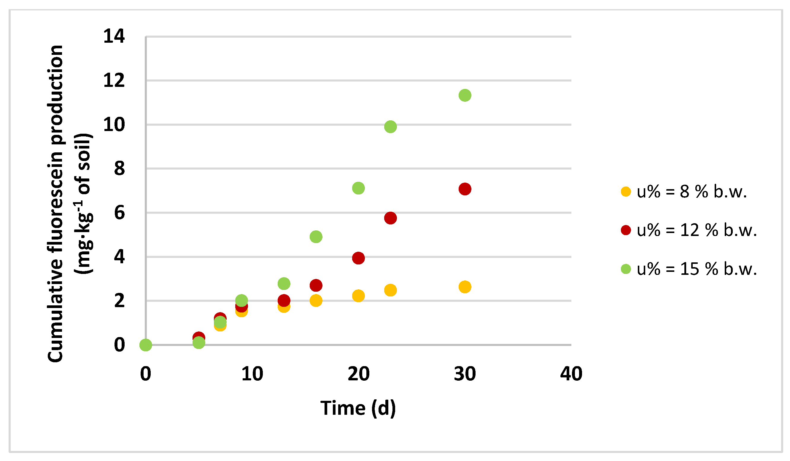
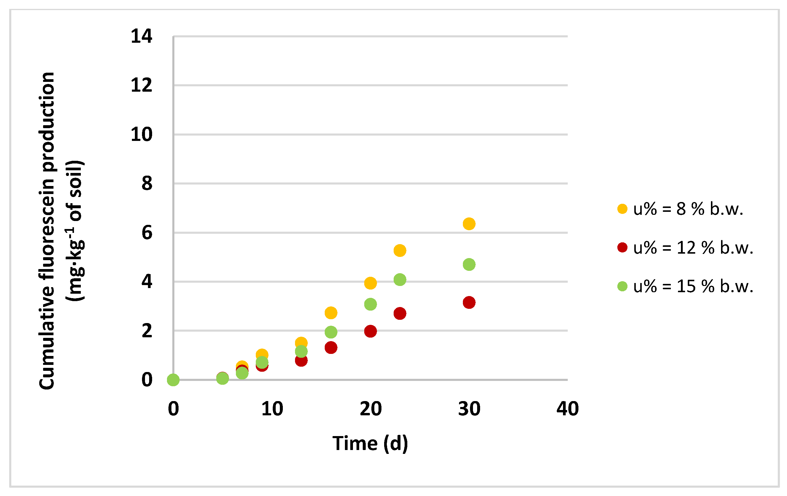
In general, it was evident that in all the microcosms, the fluorescein production started at about t = 5 days, very probably due to the time required for microbial acclimatization.

The graphs show that the fluorescein production was strongly influenced by the carbon to nitrogen ratio (C/N) and water content (u%) in the microcosms.

In the microcosms with the extreme values of C/N, namely 60 and 300, the microbial activity was reduced compared to other microcosms. This was mainly due to excessive or insufficient concentrations of nitrogen.

In addition, the water content influenced microbial growth, and the highest activity occurred with u% = 8% b.w. and u% = 12% b.w., except for the microcosms with C/N = 120, where the maximum fluorescein production (11 mg·kg⁻¹ of soil) was with u% = 15% b.w.

The highest production (12 mg·kg⁻¹ of soil) was achieved in the microcosm with C/N = 180 and u% = 12% b.w.

Table 4. Cumulative fluorescein production in 30 days.

Microcosm No.	u% (By Weight)	C/N Ratio	Cumulative Fluorescein Production (mg·kg−1 of Soil)
1	8	60	3
2	8	120	3
3	8	180	10
4	8	300	6
5	12	60	1
6	12	120	7
7	12	180	12
8	12	300	3
9	15	60	1
10	15	120	11
11	15	180	5
12	15	300	5

summarizes the cumulative fluorescein concentrations that were produced in 30 days by every tested microcosm.

3.2. Diesel Oil Removal Efficiency

All microcosms were set up with an initial diesel oil concentration equal to 70 g·kg⁻¹ of soil, and the pollutant concentration was monitored along the test.

In Figure 5, the percentage of removed contaminant is reported for microcosms with C/N = 60 and 300 after 35 days. Each value is the average derived from twice-replicated analyses on two extracts.

The findings showed that a limited amount of pollutant was removed, in both C/N ratios, independently of the water content.

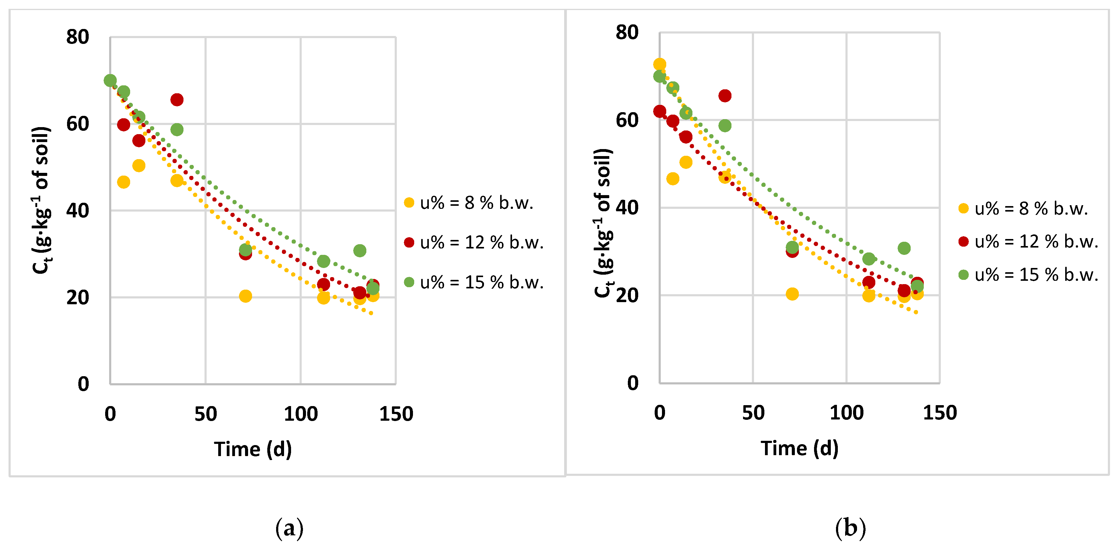
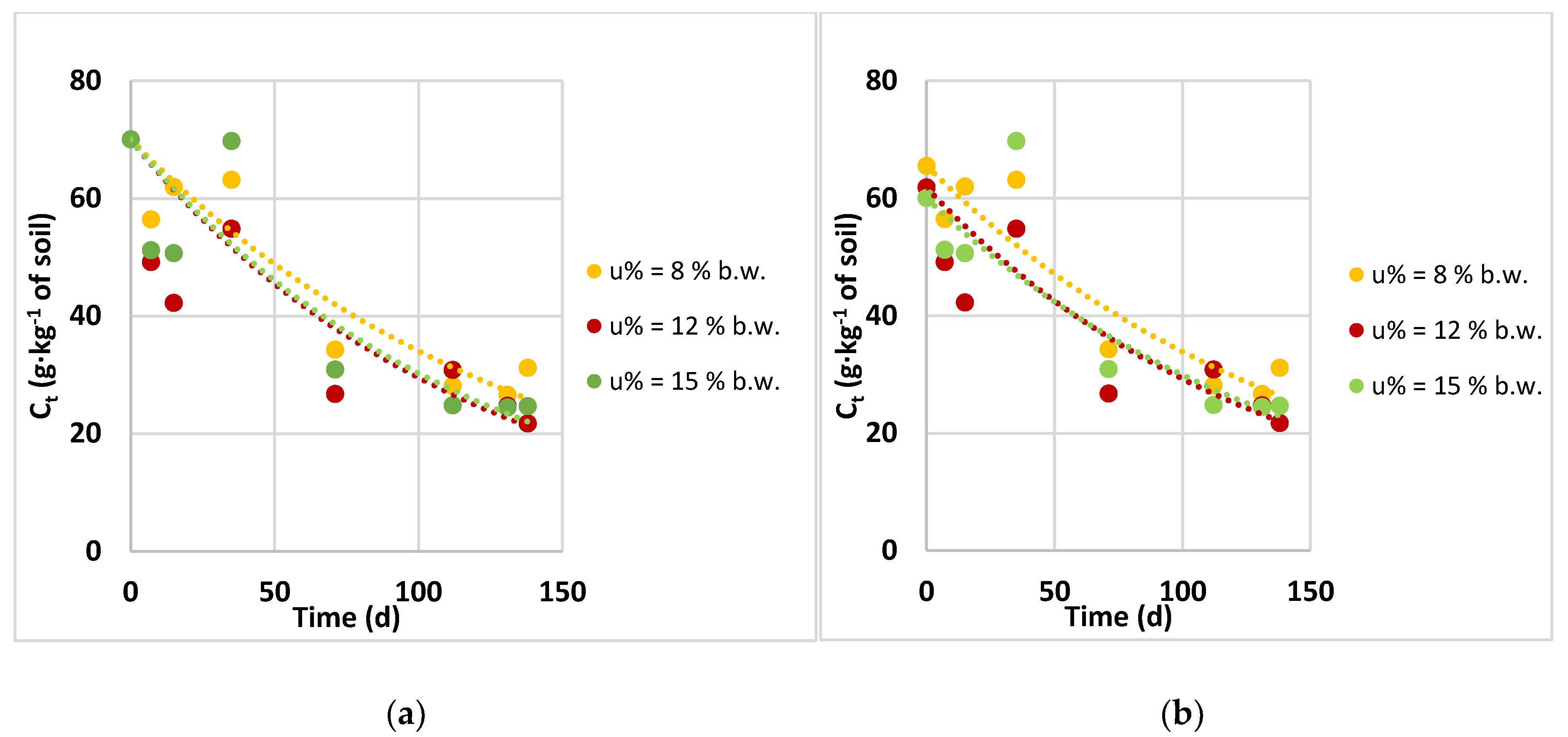
Figure 6 and Figure 7 report the monitoring of removed diesel oil by microcosms with C/N = 120 and C/N = 180, respectively. For these results, each value is the average derived from twice-replicated analyses of two extracts.

As previously mentioned, the pollutant removal efficiency was calculated considering (a) C₀ = 70 g·kg⁻¹ of soil and (b) C₀ measured by analysis.

In these tests, the diesel oil removal was evident from the start, even if appreciable results could be found after about two months.

The data showed that in the first month, the removal was influenced by the water content. Moreover, in the first 7 days for both C/N ratios, the water content that gave the highest removal result maintained this position for the entire test duration:

• after 7 days, the microcosm with u% = 8% b.w. and C/N = 120 had the highest percentage of removed diesel oil and this trend continued throughout the test;
• for microcosms with C/N = 180, the highest removal was always achieved with u% = 12% b.w.

These data proved that the biostimulation process is efficient when right conditions are adopted.

The effect of water content was evident in the first days, whereas in the last run period, the percentage of removed diesel oil was similar for all microcosms with the same C/N ratio.

In general, the data trends showed that:

• for both C/N ratios, after t = 70–75 days, the removal efficiency grew slowly: this is a feature to be considered for real-scale applications, in order to reach a compromise between long remediation times and achieved removal;
• for C/N = 180, the removal efficiency was always lower than for C/N = 120.

3.3. Kinetic Modeling

As explained in Section 2.5, in each microcosm, the initial diesel oil concentration was also measured, with the aim of detecting differences from the theoretical value of 70 g·kg⁻¹ of soil.

As already done for the diesel oil removal, kinetic modeling was done twice, in order to evaluate the influence of initial diesel oil concentration, C₀, using:

(a)

theoretical concentration calculated on the base of spiking amount and equal to 70 g·kg⁻¹ of soil;

(b)

experimental concentration of microcosm samples measured at t = 0 on soil samples.

3.3.1. First-Order Reaction Rate

Figure 8a,b shows the first-order kinetics for microcosms with C/N = 120 and with the double evaluation of the initial diesel oil concentration, as explained in Section 2.5.

The data were fitted rather well by the first-order model and R² was about 0.90, except for the microcosm with u% = 8% b.w., as shown in

Table 5. First-order reaction rate constants and half-life times for microcosms with C/N = 120.

	u% (By Weight)	First-Order Model k (d−1)	R2	t1/2 (d)
Theoretical C0	8	0.0115	0.77	60
	12	0.0091	0.92	76
	15	0.0080	0.92	89
Experimental C0	8	0.0115	0.75	60
	12	0.0080	0.91	76
	15	0.0082	0.92	85

.

The half-life times were calculated using Equation (9), and the values are reported in Table 5.

It was possible to observe that t_1/2 values were in the range of 60 to 89 days, which agrees with the percentages of diesel removal and with a previous study carried out using the same soil and pollution, although if with different C/N ratio [9].

Figure 9a,b shows the findings for microcosms with C/N = 180.

The kinetic constants and the R² values are given in

Table 6. First-order reaction rate constants and half-life times for microcosms with C/N = 180.

	u% (By Weight)	First-Order Model k (d−1)	R2	t1/2 (d)
Theoretical C0	8	0.0072	0.88	96
	12	0.0086	0.70	82
	15	0.0084	0.83	83
Experimental C0	8	0.0066	0.90	105
	12	0.0074	0.84	94
	15	0.0070	0.84	99

. The data approximation was fine in both cases, but the kinetic rate constants differed due to the influence of initial diesel oil concentration.

Table 6 also shows the half-life times for these microcosms.

3.3.2. Second-Order Reaction Rate

The data fitting with the second-order model is shown in Figure 10 and Figure 11, respectively, for microcosms with C/N = 120 and C/N = 180. As in the previous case, the modeling was done both considering the initial diesel oil concentration, equal to 70 g·kg⁻¹ of soil, and measuring the initial concentration by analysis.

With this model, the two cases gave very similar results for k value, as shown in

Table 7. Second-order reaction rate constant and half-life time for microcosms with C/N = 120.

	u% (By Weight)	Second-Order Model k (kg of soil·g−1·d−1)	R2	t1/2 (d)
Theoretical C0	8	0.0003	0.85	48
	12	0.0002	0.95	71
	15	0.0002	0.90	71
Experimental C0	8	0.0003	0.85	46
	12	0.0002	0.93	81
	15	0.0002	0.90	71

for C/N = 120, and in

Table 8. Second-order reaction rate constant and half-life time for microcosms with C/N = 180.

	u% (By Weight)	Second-Order Model k (d−1)	R2	t1/2 (d)
Theoretical C0	8	0.0002	0.90	71
	12	0.0002	0.81	71
	15	0.0002	0.90	71
Experimental C0	8	0.0002	0.90	76
	12	0.0002	0.85	81
	15	0.0002	0.90	83

for C/N = 180.

The half-life times were determined using Equation (9) and, as already discussed, this parameter depended just on the initial diesel oil concentration.

Table 7 and Table 8 report that the tested microcosms gave very similar results for reaction rate constant. However, it was noted that the differences heavily influenced the half-life time, which became a sensitive parameter, and its use in real cases should be done with attention to avoiding incorrect or overly optimistic estimates of clean-up times.

3.4. Analysis of Variance (ANOVA) and Response Surface Methodology (RSM)

In this study, the regression analysis was done considering the influence of carbon to nitrogen ratio (C/N) and water content (u%) with respect to two parameters, namely the percentage of diesel oil removal and the fluorescein production.

3.4.1. ANOVA and RSM for Percentage of Diesel Oil Removal

The results of the two-way ANOVA done on percentage of diesel oil removal in 35 days are shown in

Table 9. Analysis of variance (ANOVA) for percentage of diesel oil removal.

	SS	Df	MS	F	p
u%	0.005	2	0.004	0.42	0.67
C/N	0.039	3	0.013	1.27	0.37
Error	0.06	6	0.01
Total	0.108	11

SS = sequential sum of squares; Df = degrees of freedom; MS = mean squares; F = Fischer’s variance ratio; p = probability value.

.

Both the u% and C/N variables were statistically different in the studied confidence level. Considering the F and p parameters, the C/N effect on the objective variable (pollutant removal) was greater than that of water content.

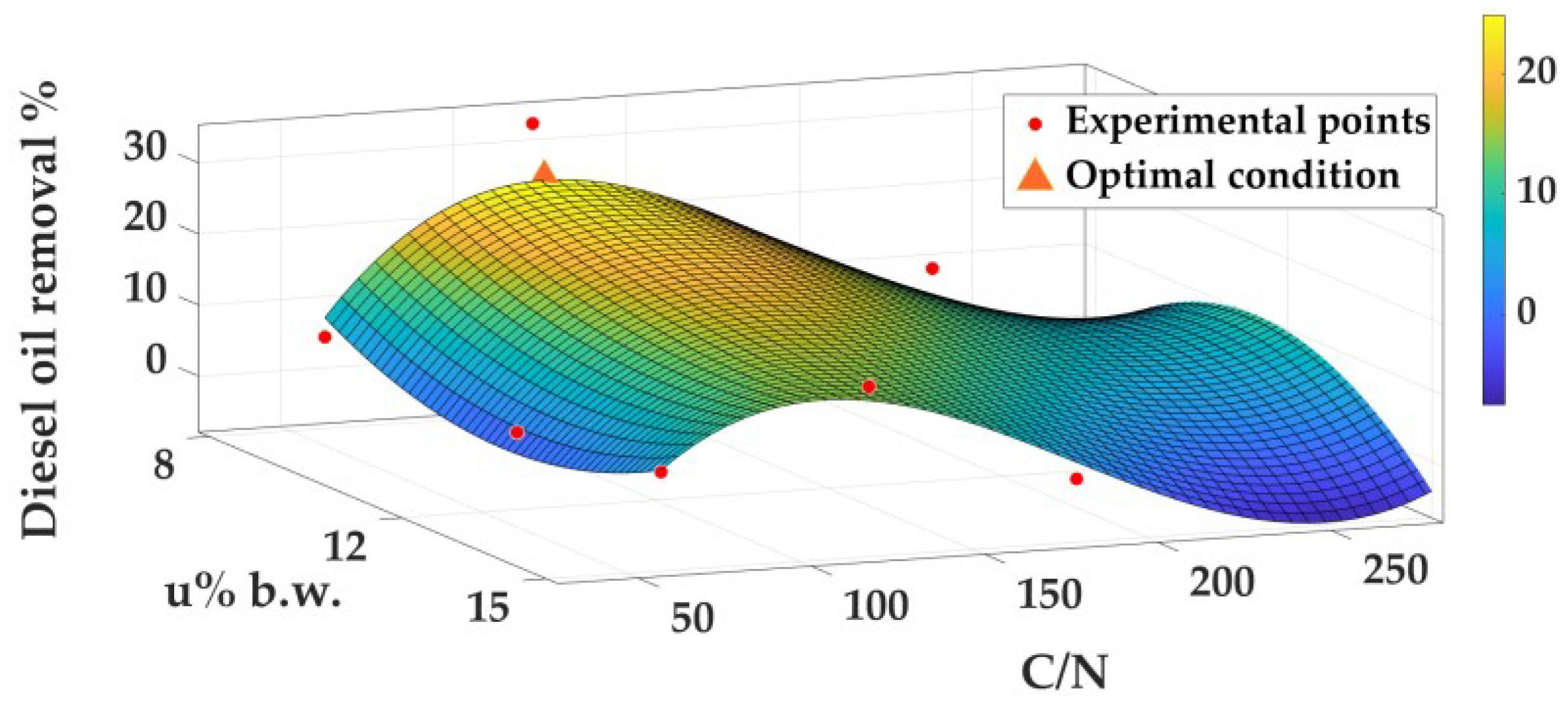
The third-degree polynomial regression was:

$$\begin{array}{c}\%\mathrm{removed}\mathrm{diesel}\mathrm{oil}=\\ 50.28-21.36{\mathrm{x}}_1+1.011{\mathrm{x}}_2+1.029{\mathrm{x}}_1^2+0.1244{\mathrm{x}}_1·{\mathrm{x}}_2-0.01006{\mathrm{x}}_2^2+\\ -0.007591{\mathrm{x}}_1^2·{\mathrm{x}}_2+0.0001458{\mathrm{x}}_1·{\mathrm{x}}_2^2+0.00001472·{\mathrm{x}}_2^3\end{array}$$

(11)

where x₁ is the water content (u%) and x₂ is the carbon to nitrogen ratio (C/N).

Considering the linear terms, the water content negatively influenced the diesel degradation (β₁ = −21.36), while the nutrient concentration had a positive effect (β₂ = 1.011). The second- and third-order terms were very small and could be considered negligible.

The combined effect of the two variables was positive (β₅ = 0.1244), but the value was small; therefore, this term can be considered negligible, too.

The same results were obtained by Lahel et al. [17]. They did an experimental design to evaluate the effects of diesel concentration, moisture content, and biomass dose on amount of removed diesel oil and CO₂ produced during the process. The study was carried out with 25 g of soil polluted with diesel oil concentration in the range of 5000 to 15,000 mg·kg⁻¹ of soil.

The response surface is shown in Figure 12.

It is evident that a maximum occurred in the area C/N = 100–180 and u% = 8%–10% b.w. By calculation, the theoretical optimum was identified: after 35 days, the maximum percentage of removed diesel oil was 24.9%, with u% = 8% b.w. and C/N ratio = 123.

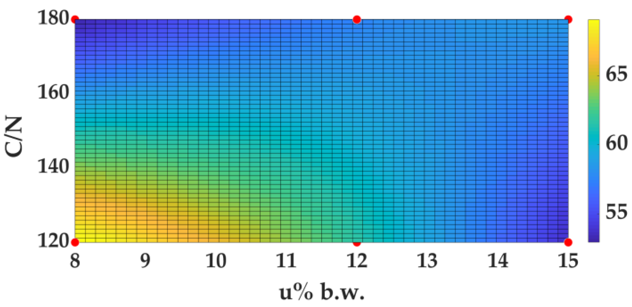
Deepening the analysis only for microcosms with C/N = 120 and C/N = 180, it was possible to monitor the yellow area’s variation throughout the test (Figure 13, Figure 14, Figure 15 and Figure 16). It was noted that the greatest percentage of diesel was removed in the space C/N = 120–130 and u% = 8%–10% b.w. After 138 days, the amount of pollutant was reduced by 70% in all microcosms with C/N = 120, while in the microcosms with C/N = 180, the diesel oil removal was still heavily influenced by the water content.

3.4.2. ANOVA and RSM for Cumulative Fluorescein Production

An analysis of variance was also done for the fluorescein production, again to evaluate the influence of u% and C/N ratio on the microbial activity. The analysis was done at t = 30 days.

It was shown that the concentration of nutrients influenced the amount of fluorescein produced, while the effects of water content were almost negligible. This was proven by the F and p values given in

Table 10. ANOVA for fluorescein production.

	SS	Df	MS	F	p
u%	0.86	2	0.43	0.036	0.96
C/N	88.66	3	29.55	2.472	0.16
Error	71.73	6	11.95
Total	161.25	11

SS = sequential sum of squares; Df = degrees of freedom; MS = mean squares; F = Fischer’s variance ratio; p = probability value.

. For C/N, the p value was lower than α; therefore, the C/N ratio was statistically important to microbial activity. For the u%, the p value was about 1; thus, the variation of water content did not affect the production of fluorescein.

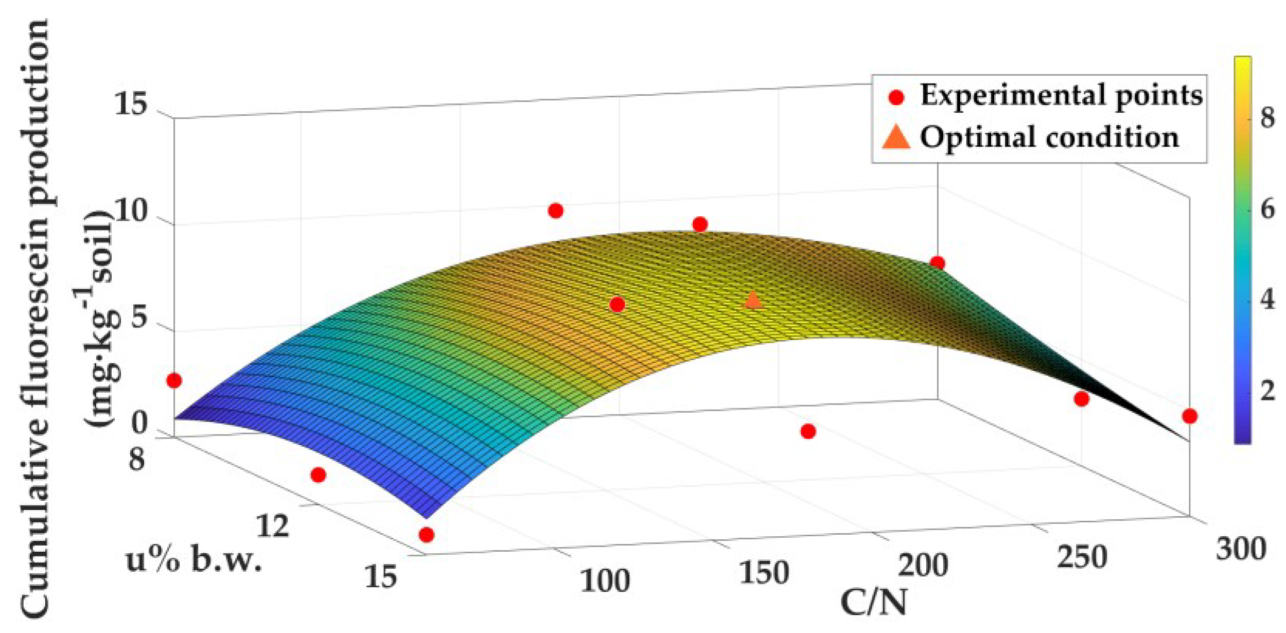
The third-degree regression polynomial was:

$$\begin{array}{c}\mathrm{Fluorescein}\mathrm{production}\left(\mathrm{mg}·{\mathrm{kg}}^{-1}\mathrm{of}\mathrm{soil}\right)=\\ -21.29+2.674{\mathrm{x}}_1+0.1879{\mathrm{x}}_2+0.1207{\mathrm{x}}_1^2-0.005597{\mathrm{x}}_1·{\mathrm{x}}_2-0.0003775{\mathrm{x}}_2^2+\\ +0.0004529{\mathrm{x}}_1^2·{\mathrm{x}}_2-0.00001929{\mathrm{x}}_1·{\mathrm{x}}_2^2+0.0000003735·{\mathrm{x}}_2^3\end{array}$$

(12)

where x₁ is the water content (u%) and x₂ is the carbon to nitrogen ratio (C/N).

Considering the polynomial coefficients, it is possible to see that the second- and third-order terms were negligible and the coefficients for water content (β₁ = 2.674) and for C/N ratio (β₂ = 0.1879) were positive. Therefore, an increase of u% and C/N ratio enhanced production of fluorescein, i.e., the microbial activity.

The response surface for the fluorescein production after 30 days is shown in Figure 17.

For microbial activity, the optimal condition occurred with a C/N ratio in the range of 180 to 220, regardless of the water content in the tested range. This means that fluorescein production was not influenced by the percentage of water content when this factor was in the range of 8% to 15% b.w.

With reference to Equation (12), the theoretical optimum on the surface was calculated; the fluorescein production was equal to 9.8 mg·kg⁻¹ of soil, with u% = 13.3% b.w. and C/N ratio = 182.

3.5. Open-Ended Coaxial Cable Measurements

Figure 18a,b shows the real and imaginary components of soil versus the frequency of the applied signal. They refer to the microcosm with C/N ratio = 120 and water content = 8% b.w. The values measured at t = 0 are shown in blue, and the ones at t = 130 days in red.

The main information that can be inferred from observing Figure 18a,b is that a significant decrease in complex permittivity happened at all investigated frequencies. This could evidence the loss of diesel compounds by means of biodegradation, or a slight loss in water content, although the microcosms were sealed for the most of the time (namely, except when they were mixed to provide oxygen). It is interesting to notice that the imaginary part decreased after bioremediation, especially at low frequencies, probably indicating a loss in the material conductivity due to the depletion of nutrient salts.

4. Discussion

The experimental tests on microcosms polluted with diesel oil at a constant concentration (70 g·kg⁻¹ of soil) but with different water contents (u%) and carbon to nitrogen ratios (C/N) were designed according to the factorial analysis, to get experimental results useful

• to model the process kinetics;
• to study the interactions between these two operative factors, u% and C/N;
• to optimize the operative conditions to remove pollution in a reasonable time and with good efficiency

with limited number of tests but exploiting their links to highlight their interactions, if any.

In biological processes, as well as in chemical ones, kinetic modeling is one of the pillars used to plan real processes. Its identification must be derived from experimental tests done at smaller scale than the future application one. In this study, the reaction rate was modeled with a first- and second-order model, to check whether one model was more reliable and robust than the other. Given that the squared regression coefficient, R², of a model reflects the variability of the target parameter, with reference to this work, Table 5, Table 6, Table 7 and Table 8 report this quantity representing the variability of the residual diesel oil concentration in soil for each run changing the operative factors (u% and C/N). In general, the R² values were high in both models, confirming that they were both satisfactory for this application. This has also been shown by other authors [12,30]. Comparing the R² values, the second-order model seemed to give lower variability, especially when the half-life time, t_1/2, was longer. However, at a more careful check, this was also shown by the first-order model. This finding could mean that removal efficiency is estimated with better reliability when reaction kinetics are slower, i.e., when t_1/2 is longer.

Regarding the half-life time, t_1/2, the findings were in line with results achieved by other authors [15,29,31]; this parameter has a particular relevance when study previsions must be transferred to in situ application, i.e., where its value has influence on the management remediation plan.

The analysis of variance allowed us to estimate the influence and interactions of the operative parameters on diesel oil removal efficiency and fluorescein production (indirect measurements of microbial activity). The regression model done at t = 35 days and given by Equation (11) showed that only the linear effects of u% and C/N and the quadratic effect of u% were significant for the removal efficiency; specifically, the water content had a negative effect (β₁), while the other significant interactions, shown by β₂ and β₃, were positive. The additional ones, from β₄ to β₇, had no influence. For the microbial activity, depicted by fluorescein production at t = 30 days (Equation (12)), the effects to be considered were still the same as for diesel oil removal efficiency (β₁, β₂, and β₃), even if with different trends (they were all positive).

Finally, the response surface methodology was applied to optimize the objective parameters already considered in the analysis of variance: diesel oil removal efficiency and fluorescein production. In both cases, the graphical result was a curved surface, due to cubic regression.

For η-value, the findings clearly identified the zones where the parameter was higher than in the others; in these zones, the optimum could be found. Using chromatic representation, these results were rather evident. For the fluorescein production, the response surface showed that when the water content was in the range of 8% to 15% b.w., this parameter had limited effect.

As we have demonstrated, statistical analysis by analysis of variance and response surface methodology can be adopted successfully for experimental analysis of the degradation process at a laboratory scale. The findings confirm the applicability of the tool to complex systems, as already proposed by other authors [16,17,18,19,20,21] in similar studies and with similar conditions.

The second challenging issue was to check the reliability of fast and accurate technology to monitor the process itself. In a previous study, tests using a time domain reflectometer (TDR) were adopted to measure the dielectric properties of the samples. In those cases, even if the approach seemed promising, some inaccuracies made the results ambiguous in terms of the relationship between the biomass activities and the observed geophysical parameters. The open-ended coaxial cable could, in theory, overcome some of the previous problems, as discussed by Skierucha et al. [32], who carried out a detailed comparison of TDR and open-ended coaxial probes applied to non-contaminated agricultural soils. The two kinds of probes gave highly correlated results in determining the real part of permittivity at frequencies around 1 GHz. However, the open-ended coaxial cable investigated the frequency-dependent imaginary part with much more detail. It provided a wide frequency spectrum of analysis, in which different polarization phenomena influenced the complex dielectric permittivity.

We did not find in the literature the use of open-ended coaxial cables in monitoring of bioremediation of contaminated soils, while these probes are commonly used in other application fields to evaluate biological substances or tissues [33].

In fact, the use of an open-ended coaxial cable to monitor the effects of biodegradation on dielectric properties of soil gave interesting results, because of the capability to monitor both the real and the imaginary part in a wide frequency range. Variations in diesel oil content can significantly affect the real part of the dielectric permittivity of a soil matrix, as also observed by Comegna with TDR [34], and by Godio with an open-ended coaxial cable [25] in non-bioremediated contaminated soils. Instead, the variations in the imaginary component are related to progressive changes in the pore water chemistry due to biological phenomena. The latter are observed especially at low frequencies (<1 GHz): after 130 days of bioremediation, the imaginary component at 200 MHz decreased to near-zero values, indicating that the conductivity of pore water decreased during the process. Fluctuations in pore water conductivity of a soil under bioremediation were also observed in Mori et al. [35].

The use of an open-ended coaxial cable is a fast method to estimate both electrical permittivity and conductivity. The application of this technology to soil bioremediation is a new research field, and these initial experiments allowed us to focus on different phenomena of the degradation process, such as hydrocarbon depletion or salt depletion. However, the correlation between biological findings and geophysical ones remains a challenge for researchers.