1. Introduction
Economic load dispatch (ELD) is known as a means of lowering fuel costs for electricity generation in thermal power plants. In power system operation, the main purpose of the ELD problem is to allocate the power output of each power plant continuously, while observing the conditions such as fuel consumption characteristics, capacity of each generator, technical requirements in the system, and total demand of all loads. The objective function of this problem is to reduce the values of a quadratic function, a non-convex function, or a non-smooth function as much as possible. So, the complexity of the problem is partially dependent on the complexity level of the objective function. Basically, a solution can be regarded as an acceptable operation method if all constraints are exactly met. Thus, complex of constraints is also a challenge for the complexity level of the ELD problem. Due to these challenges, approximately all studies have focused on the objective function and the considered constraints to demonstrate their method’s efficiency.
In the later years of the previous century, traditional methods were effectively applied to solve the ELD problem with acceptable results. These methods are the lambda-iteration method (LIM) [
1], gradient method (GM) [
1], hierarchical method (HM) [
2], Lagrange relaxation (LR) [
3], linear programming technique (LPT) [
4], Newton’s method (NM) [
1], and fast Newton Raphson method (FNM) [
5]. Traditional methods have the advantage of using a small number of iterations, and results are the same for different runs because they are deterministic methods. However, traditional methods have to take the partial derivative in the process of finding solutions. So, these methods have some restrictions if they solve the ELD problem for complex systems, for example, those with non-smooth shape objective functions.
Another method group that appeared after these traditional methods and has also been successfully applied to solve the ELD problems is composed of the artificial neural network (ANN)-based methods. This group includes the Hopfield neural network (HNN) [
6], adaptive Hopfield neural network (AHNN) [
7], new Hopfield model (NHM) [
8], enhanced augmented Lagrange Hopfield network (EALHN) [
9], and augmented Lagrange Hopfield network (ALHN) [
10]. ANN-based methods perform better than traditional methods by combining the Lagrange function and Hopfield network. However, these methods, like traditional methods, struggle with complex objective functions.
In contrast to the above methods, evolutionary algorithms (EAs) and improved evolutionary algorithms (IEAs) have been popularly applied to solve the ELD problem with complex systems. These types of algorithms include the improved genetic algorithm (IGA) [
11], real-code genetic algorithm (RCGA) [
12], new RCGA (NRCGA) [
12], evolutionary strategy optimization (ESO) [
13], improved differential evolution (IDE) [
14], differential evolution (DE) [
15], hybrid integer coded differential evolution and dynamic programming (HDE-DP) [
16], and stud differential evolution (SDE) [
17]. Among these methods, RCGA [
12] is the best because it can solve the ELD problem with valve point effects (VPEs), multi fuels (MFs), ramp rate limit (RRL), prohibited operating zones (POZs), and spinning reserve (SR), whereas IDE [
14] is the best method in terms of solving problems considering transmission losses.
Similar to IEAs, metaheuristic-based methods have been very quickly developing for solving the ELD problem, and there have been a large number of methods developed from the metaheuristic algorithms such as Particle swarm optimization (PSO) [
18], Quantum-inspired particle swarm optimization (QIPSO) [
19], Particle Swarm Optimization and Tabu Search Algorithm (DSPSO-TSA) [
20], Fuzzy and Self-Adaptive Particle Swarm Optimization (FSAPSO) [
21], Theta Particle Swarm Optimization (θ-PSO) [
22], Modified Particle Swarm Optimization (MPSO) [
23], Artificial Immune System Algorithm (AISA) [
24], Biogeography-based Optimization (BBO) [
25], Chaotic Firefly Optimization Algorithm (CFOA) [
26], Cuckoo Search Algorithm (CSA) [
27], Modified Cuckoo Search Algorithm (MCSA) [
28], One Rank Cuckoo Search Algorithm (RCSA) [
29], CSA [
30], MCSA [
31], Krill Herd Algorithm (KHA) [
32,
33], Modified Krill Herd Algorithm (MKHA) [
34], Modified Firefly Algorithm (MFA) [
35], Varying Firefly Optimization Algorithm (VFOA) [
36], Firefly Optimization Algorithm (FOA) [
37], Improved Firefly Optimization Algorithm (IFOA) [
37], Effectively Modified Firefly Algorithm (EMFA) [
38], Immune Algorithm (IA) [
39], Grey Wolf Optimization Algorithm (GWOA) [
40], Chaotic Bat Optimization Algorithm (CBOA) [
41], Exchange Market Algorithm (EMA) [
42], Antlion Optimization Algorithm (ALO) [
43,
44], and Spotted Hyena Optimizer (SHO) [
45]. Among the metaheuristic-based methods, EMFA [
38] has been tested on many systems with complicated constraints such as transmission losses, POZs, ramp rate limits, spinning reserve, and fuel consuming characteristics such as MFs and VPEs. In addition, the method has been tried for very large-scale problems with a high number of generators and a high number of control variables. The results showed that the EMFA method provided the highest quality results compared to all other methods including the FOA, PSO, DE, CSA, and genetic algorithm (GA). In summary, improved methods have a good ability to search for better optimal solutions. Conversely, these methods become complex because of the combination of the original algorithms-based developed methods and modified mechanisms.
In this paper, an improved antlion optimization algorithm (IALO) is suggested for solving the ELD problem. Constraints such as transmission losses, POZ, RRL, and SR are considered. Moreover, we take into account the consuming characteristics of MFs and VPEs. In 2015, Mirjalili [
43] suggested the antlion optimization (ALO) algorithm for solving technology problems. The ALO method has been applied for solving the ELD problem in very small-scale electricity systems considering VPEs [
44]. More research is needed to further clarify the efficiency of the ALO method. The suggested IALO method was tested on five different systems with different consuming characteristics and constraints. The results obtained by the IALO were analyzed, evaluated, and compared in other papers in the literature. The goals of the current work can be summarized as follows:
Present all the computation steps of the ALO in detail and analyze drawbacks of the method;
Discuss improved versions of the ALOs that previous studies have proposed;
Propose a highly effective modification to produce a promising solution search strategy;
Combine our proposal with a modification that was proposed in a previous work. The combination of the highly effective proposed modification and the applied modification can support the proposed IALO method in finding optimal solutions effectively and quickly;
Consider the different systems that contain complex objective functions and constraints;
Compare our proposed IALO with classic ALO. Our proposed IALO can achieve much better results than those of the ALO with the same settings for control parameters. The proposed method is better or equal to other existing methods in comparing quality of solution, but it is more robust than these methods when comparing computational steps.
The remaining parts of the paper are organized as follows:
Section 2 expresses the mathematical formulation of the ELD problem.
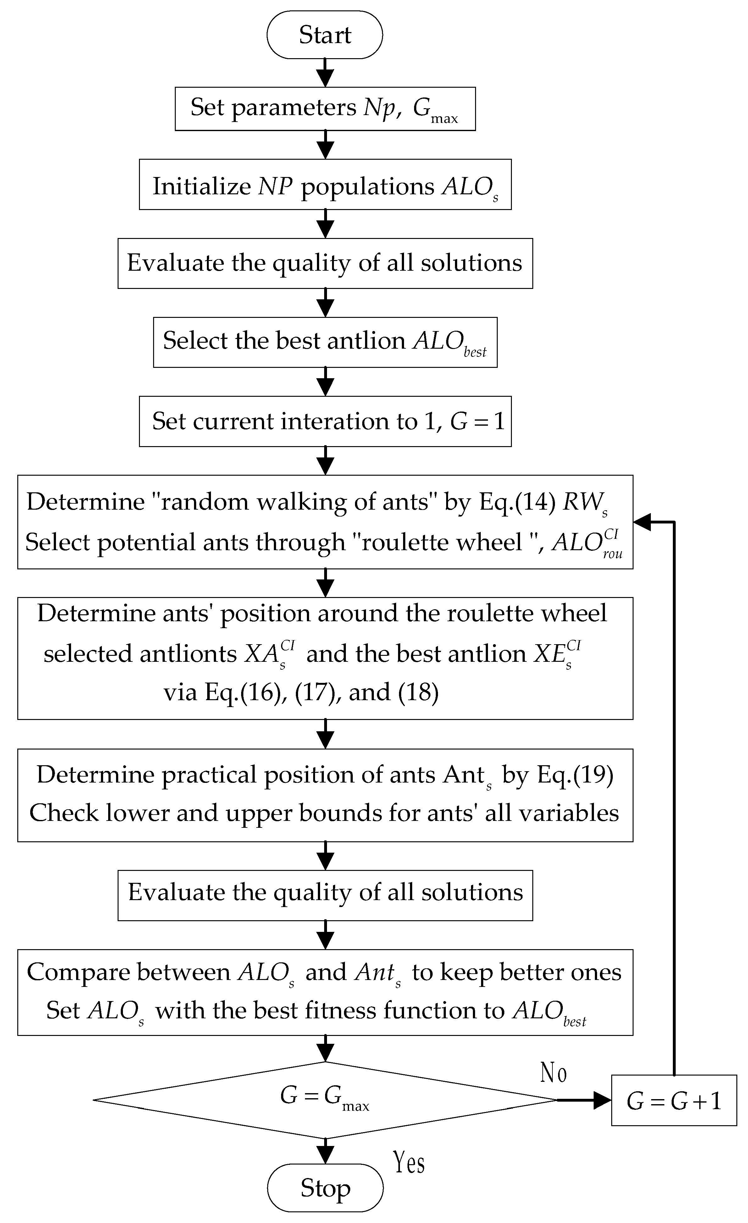
Section 3 presents the ALO and IALO methods in detail.
Section 4 shows the detailed implementation of IALO for the ELD problem.
Section 5 presents simulation results and discussion.
Section 6 summarize the achievement and conclusions of the study.
5. Numerical Results
To demonstrate the effectiveness of the proposed IALO method, four main study cases are implemented as follows:
- (i)
Consider MFs for each unit of a 10-unit system;
Case 1: Consider four load cases of 2400, 2500, 2600, and 2700 MW without VPEs;
Case 2: Consider one load case of 2700 MW with VPEs;
Case 3: Consider one load case of 2700 MW with VPEs and constraints such as SR, POZ, and RRL.
- (ii)
Consider SF for each unit of a 20-unit system supplying a 2500 MW load considering power loss;
- (iii)
Consider MFs and VPEs for the 80-unit system with a 21,600 MW load;
- (iv)
Consider SF for each unit for the 15, 30, 60, and 90-unit systems with POZ constraints.
The proposed method together with the ALO were programmed in the Matlab platform and run on a PC (Processor with 2.7 GHz, RAM with 4.0 GB). In order to investigate the real performance of the IALO method, another comparison criterion was also considered to be the number of fitness evaluations,
Nfes, which is shown in the following equation:
In the equation above, ω is the number of new solution generation times in each iteration. The IALO method has only one generation time for each iteration, so
ω is 1 for IALO while
ω is 2 for CSA [
27] and RCSA [
29]. For other methods such as FOA and IFOA in [
37],
Nfes had another model as follows:
Furthermore, we also computed the improvement of the proposed method over other compared methods by using the best cost of the compared methods and our proposed method. The improvement in % (
ic) can be obtained by the following model:
In Equation (48), values of ic can be classified into three cases in which Case 1 corresponds to positive values, Case 2 corresponds to zero values, and Case 3 corresponds to negative values. If Case 1 occurs, the suggested method is more effective than the compared method. In the case of an ic with zero value, the suggested method is as good as other ones. In contrast, Case 3 indicates the suggested method is less effective than the compared methods if the compared methods have reported valid solutions and used smaller Nfes values in Equation (47).
5.1. Comparison for Results from the 10-Unit System with Different Cost Function Characteristics
This system has ten thermal generating units with a non-smooth fuel cost function. There are three cases for this system consisting of MFs; MFs and VPEs; and MFs and VPEs under complex constraints. Data of the system are taken from [
7] for Case 1 and [
11] for Cases 2 and 3.
5.1.1. Case 1: 10-Unit Systems with MFs
The suggested IALO method was tested on four sub-cases of load demands consisting of 2400, 2500, 2600, and 2700 MW. For each case, 100 trial runs were executed to obtain results and comparisons. In order to investigate the search potential, we compared the proposed method with other methods based on the obtained results (including the best cost, minimum cost, and average cost) and the number of fitness evaluations
Nfes (which was calculated by using Equation (46) with the presence of the population size and the number of iterations). The comparison of obtained results indicated the search performance of the methods, meanwhile the comparison of
Nfes indicated the search speed of methods. For better comparison of search performance, we converted better cost into improvement in %, which was calculated by using Equation (48). Basically, methods have a better chance to reach better results if they are run with larger population sizes and more iterations. We wanted to reflect the real performance of the proposed method and so we compared the obtained results; however,
Nfes was always compared to assure a fair comparison between the proposed method and other methods. In
Table 1, a comparison is shown for the same system with four different load cases. We ignored the comparisons of the mean and maximum costs because there were four comparison cases. Furthermore, the proposed method was run by using smaller
Nfes than that of other methods. Therefore, if the proposed method can reach the same best cost as the other methods, the proposed method is more effective because it is faster. Observing the best cost indicates that the suggested method is better than the ALO method in terms of the best cost for all of load demand cases. In comparison with the ALO, the highest improvement level was 0.931%, corresponding to the case of a 2600 MW load demand, and the lowest level of improvement was 0.330% for a 2700 MW load demand. As compared to the other methods, the IALO method can reach the same result as other methods, excluding CSA [
27], which suffers from a slightly higher cost than the proposed method. For example, in the case of a load demand of 2600 MW, the best fuel cost of the IALO was 574.381
$/h. It is smaller than the 574.410 (
$/h) value for the CSA, being tantamount to 0.005%. Although, the proposed method cannot reach better cost values than the other remaining methods, the proposed method uses smaller
Nfes than all other methods excluding EALHN [
9], which is not a population-based method. In fact, the proposed method produced about 750 fitness evaluations while the other methods produced from 2000 to 20,000 fitness evaluations. The search speed of the suggested method was 2.6–26 times faster than those of the other methods. The analysis of the best cost and search speed indicates that the application of the suggested method to solve a 10-unit system with multi-fuel options is absolutely effective.
5.1.2. Case 1: 10-Unit System with MFs and VPEs
This system had ten generating units with the sum of several non-convex functions. The load demand of the test system was 2700 MW. The obtained results including the best cost, mean cost, worst cots, and standard deviation for 100 trial runs are shown in
Table 2. In addition,
Np,
Gmax,
Nfes, and
ic (%) are also reported for comparison in detail. The best cost value of the IALO method was the lowest among all compared methods, including PSO, FOA, IFOA, CSA, RCSA, and ALO. The highest improvement was 6.124% as compared to the FOA method and the lowest improvement was 0.004% as compared to the RCSA method. Clearly, FOA was not a powerful method for the system and it was modified and changed into IFOA with much better results with an
ic of 0.007% even though the IFOA used only half of the number of fitness evaluations. CSA [
27] used the highest number of fitness evaluations, at 10,000, among all compared methods, but it could not reach the best solution and, therefore, the proposed method reached improvement over that method with 0.005%. The proposed method reached the best solution, but it used the highest number of fitness evaluations, excluding the comparison with CSA. The results show that it is hard to improve the results for the system with a small number of fitness evaluations, similar to the other compared methods. However, the running time of the proposed method was small compared to those of the other methods. Consequently, the proposed method is a potential method for 10-unit system taking multi-fuel options and vale point loading effects into account.
5.1.3. Case 3: 10-Unit System with MFs, VPEs, and Other Complexity Constraints
Next, we added several complex constraints such as spinning reserve, generating capacity, POZs, and ramp rate into the 10-unit system with MFs and VPEs.
Table 3 lists the obtained results for a 2700 MW load demand and reports
Nfes and
ic for better comparisons. The IALO method was better than RCGA, FOA, IFOA, and ALO methods because the best cost of the IALO method was the smallest. The highest and the lowest improvement of the suggested method over these methods was, respectively, 7.304% and 0.005%. The values of
Nfes from all methods indicates that the proposed method was one of the fastest methods with 3000 fitness evaluations, whereas the slowest method used 6000 fitness evaluations. However, the best cost of the IALO is slightly higher than that of the NRCGA method with −0.001%. This number shows that the best performance was not achieved by the proposed method, but our method is still a very efficient one. In fact, NRCGA reached the lowest cost, but the application of that method was only for the study cases with multiple fuels and VPEs, whereas the proposed method was implemented for different constraint types, different fuel types, and very large scale systems with 80 units and 90 units.
5.2. Implementation of the Suggested Method on a 20-Unit System Considering Transmission Loss
This section presents the comparison of the best cost,
CPU, and
Nfes from the proposed IALO and other methods with a load power of 2500 MW. Data of this system was taken from [
39]. The obtained results for this study are given in
Table 4. When compared to IA [
39], the suggested method was more powerful for all criteria, such as the best cost with an
ic % of 0.016%,
CPU, and
Nfes. The suggested method was much faster when comparing 4500 and 20,000 fitness evaluations. The outstanding performance cannot be seen when the proposed method was compared to the other remaining methods, but the proposed method was still evaluated to be more powerful. In fact, the best costs of RCSA [
29], CBOA [
41], and ED-SHO [
45] were equal to that of the suggested method, but RCSA, CBOA, and ED-SHO methods used higher values for
Nfes equaling 10,000, 12,000, and 100,000, respectively. These values were much higher than the 4500 of the IALO. Other values such as the mean cost and the standard deviation reveal the stable search ability of the proposed method since the mean cost and the best cost of the proposed method are approximately the same as those of the other methods, and the standard deviation is nearly zero. The proposed method used the lowest number of fitness evaluations, but it reached the same best cost and the most stable ability. As a result, it can be concluded that the IALO is a potential method for the system with 20 units considering quadratic fuel cost function and power loss constraint.
5.3. The Implementation of the Suggested Method on an 80-Unit System
In order to demonstrate the efficiency of the suggested method, a larger system with 80 thermal generating units with multi-fuel options and vale point loading effects was considered [
11]. The load demand of the system was 21,600 MW. The study case was an expanded case of the 10-unit system with MFs and VPEs in
Section 5.1.2 above. Compared methods had the same challenge of a discontinuous objective function and a high number of control variables. The comparisons with CSA, RCSA, and ALO are shown in
Table 5. Because it is a complicated study case, the improvement of the proposed method over its conventional method can be seen clearly. The
ic over ALO was 0.194%, but this value is much smaller compared to those of CSA and RCSA, where the values of
ic were only 0.01% and 0.005, respectively. The insignificant improvement can be understood because the two methods were run by using 132,000 fitness evaluations while the proposed method was run by using only 80,000 evaluations. For this case, the proposed method was the fastest method and reached the best solution. So, it is a very efficient method for a large-scale, 80-unit system considering MFs and VPEs.
5.4. The Implementation of the Suggested Method on 15, 30, 60, and 90-Unit Systems with POZ Constraints
This section investigates the achievement of the suggested method on four cases of 15, 30, 60, and 90 units. Data of the study cases were taken from [
6]. SR of the system was 200 MW for the case with 15 units and its increase was directly proportional to the number of units for the other remaining systems. Control parameters selection for ALO, the proposed method, and other compared methods are given in
Table 6. Obtained results are reported in
Table 7.
Table 7 indicates that the IALO was highly superior to ALO method in terms of the best cost with very high improvement levels, such as 0.43% for a 15-unit system, 0.19% for a 30-unit system, 0.11% for a 60-unit system, and 0.15% for a 90-unit system. The saving cost percentage was significant for the systems because the two methods had the same control parameters selection, as shown in
Table 6. The comparisons with CSA and RCSA do not show a benefit of the proposed method, since IALO was only slightly better than these methods for the case of a 90-unit system, whereas the other cases were similar, excluding the comparison with RCSA for a 15-unit system. The RCSA showed effective cost but did not show optimal generation for verification. The
Np,
Gmax, and
Nfes in
Table 6 indicate that the proposed method is much faster than CSA and RCSA for the 15- and 30-unit systems. The proposed method used 2000 and 20,000 fitness evaluations for the 15- and 30-unit systems, respectively, but CSA and RCSA used 12,000 and 48,000 fitness evaluations, respectively. However, for the two large-scale systems with 60 units and 90 units, the proposed method was slower because it used 80,000 and 160,000 fitness evaluations, respectively, whereas CSA and RCSA used 60,000 and 72,000 fitness evaluations, respectively. The
Nfes and the best cost reveal that the proposed method was very effective for small-scale systems with 15 TGUs and 30 TGUs, but was less effective for large-scale systems with 60 and 90 TGUs.
5.5. Investigation of the Real Performance of IALO and ALO
The results from the suggested method and ALO method are summarized in
Table 8. In all the cases of
Table 8, the best cost of the IALO was always smaller than that of the ALO. Moreover, the time to run the program of the IALO method was always lower than that of the ALO method for all cases. The
ic of 0.43% was the highest improvement of IALO over ALO, corresponding to the case of 15-units with POZ for a 2650 MW load demand. In contrast, 0.0001% was the smallest improvement of the suggested IALO over the ALO, corresponding to the case of a 20-unit system considering transmission loses for a 2500 MW load demand. However, in this case, ALO used
Nfes = 9000 while IALO used only half of that quantity, i.e., 4500. To demonstrate the superiority of the IALO more persuasively, the convergence characteristics of the IALO and ALO are plotted in
Figure 2,
Figure 3,
Figure 4,
Figure 5 and
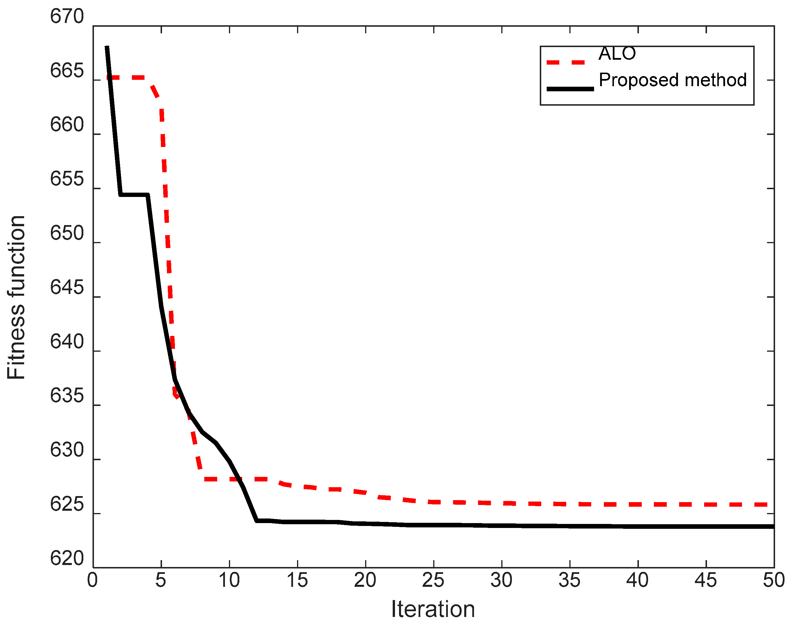
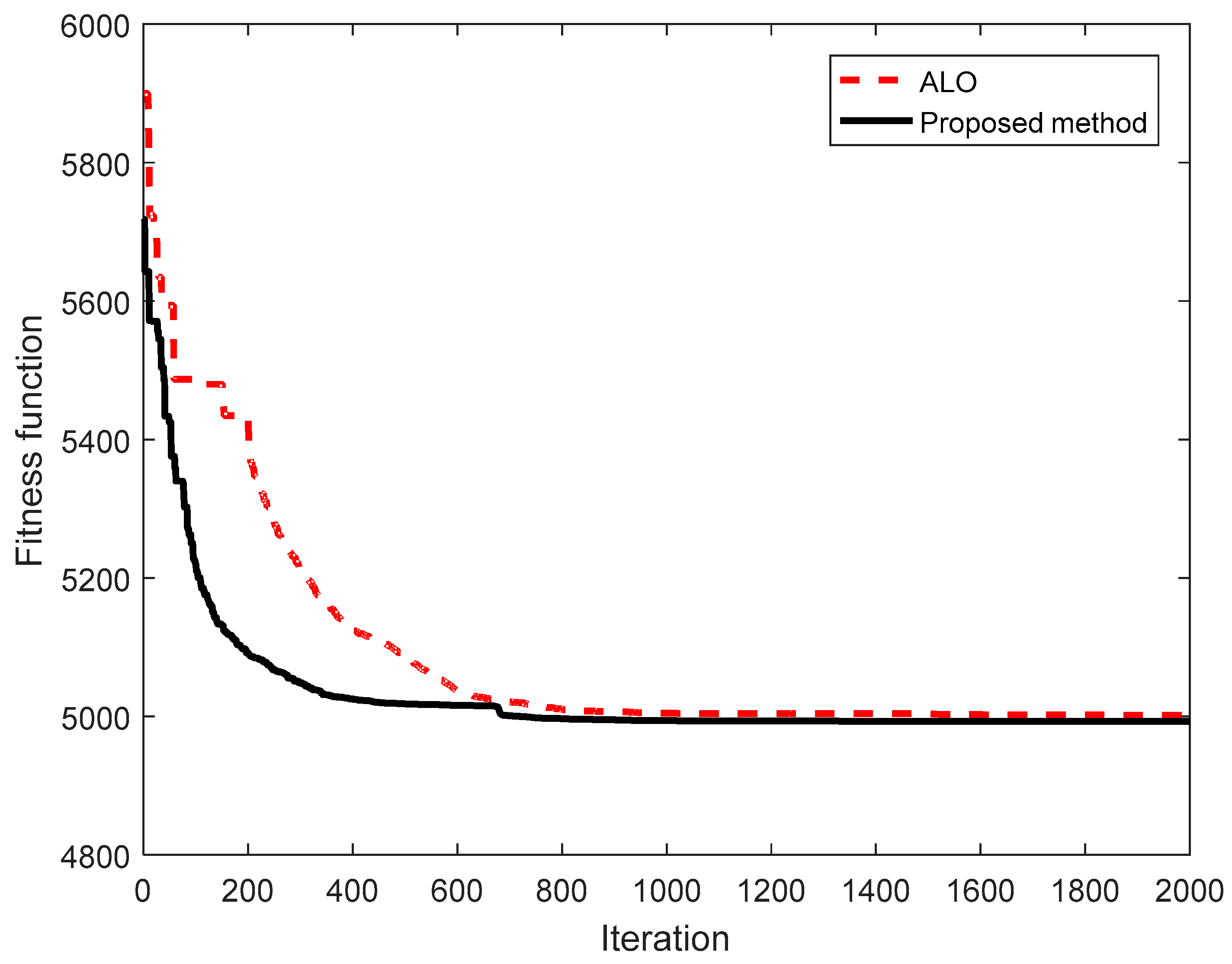
Figure 6 for different cases from the sections above. Through the figures, it can be seen that the IALO converged faster than the ALO after half of the number of iterations, or even fewer than half. For instance,
Figure 2 shows the IALO reached a solution close to the best solution at the fifteenth iteration, whereas the solution of the ALO at the fiftieth iteration was far from the obtained solution of the IALO. In
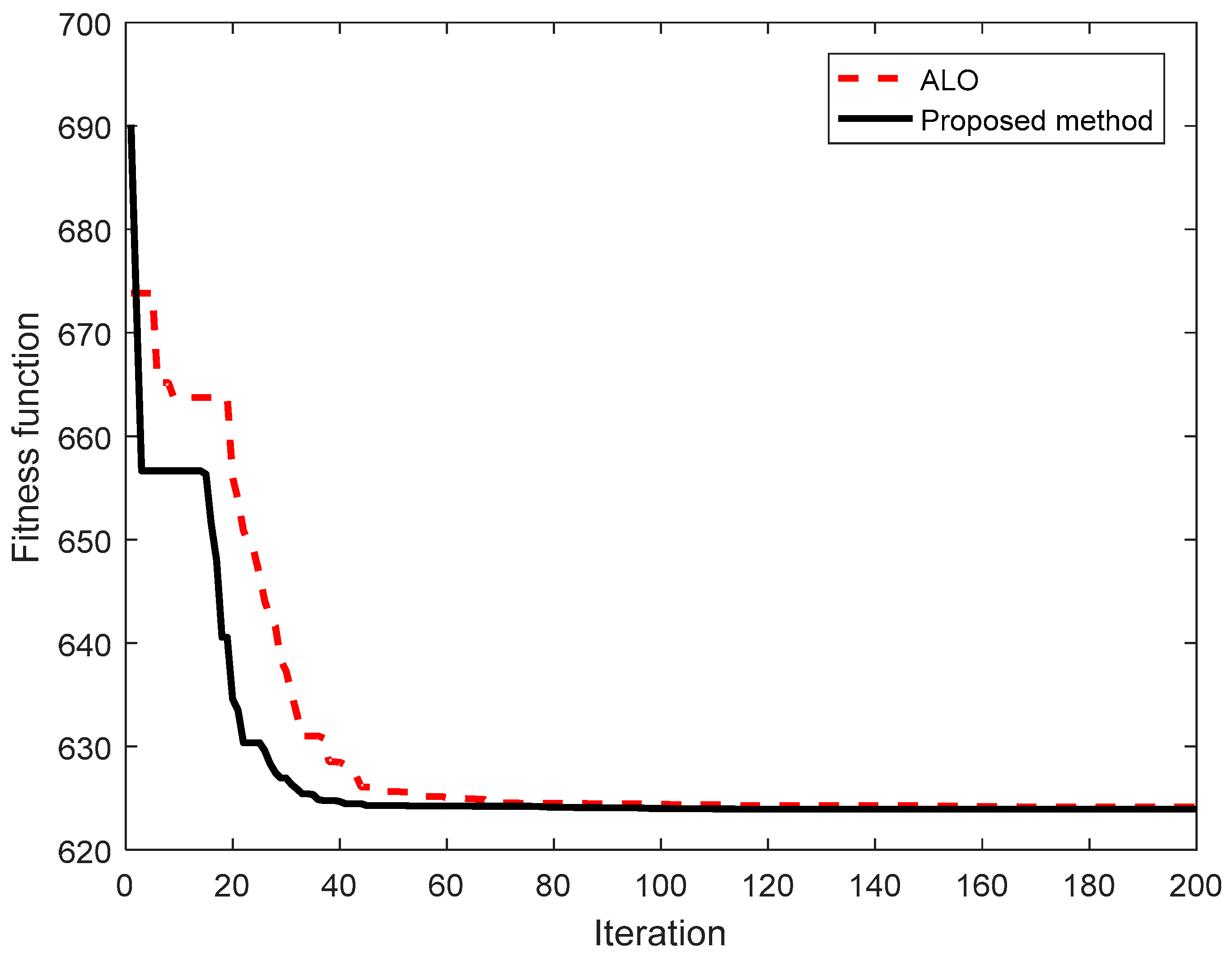
Figure 3, the solution of the IALO at the sixtieth iteration was much more effective than the solution of the ALO at the 200th iteration. Furthermore,
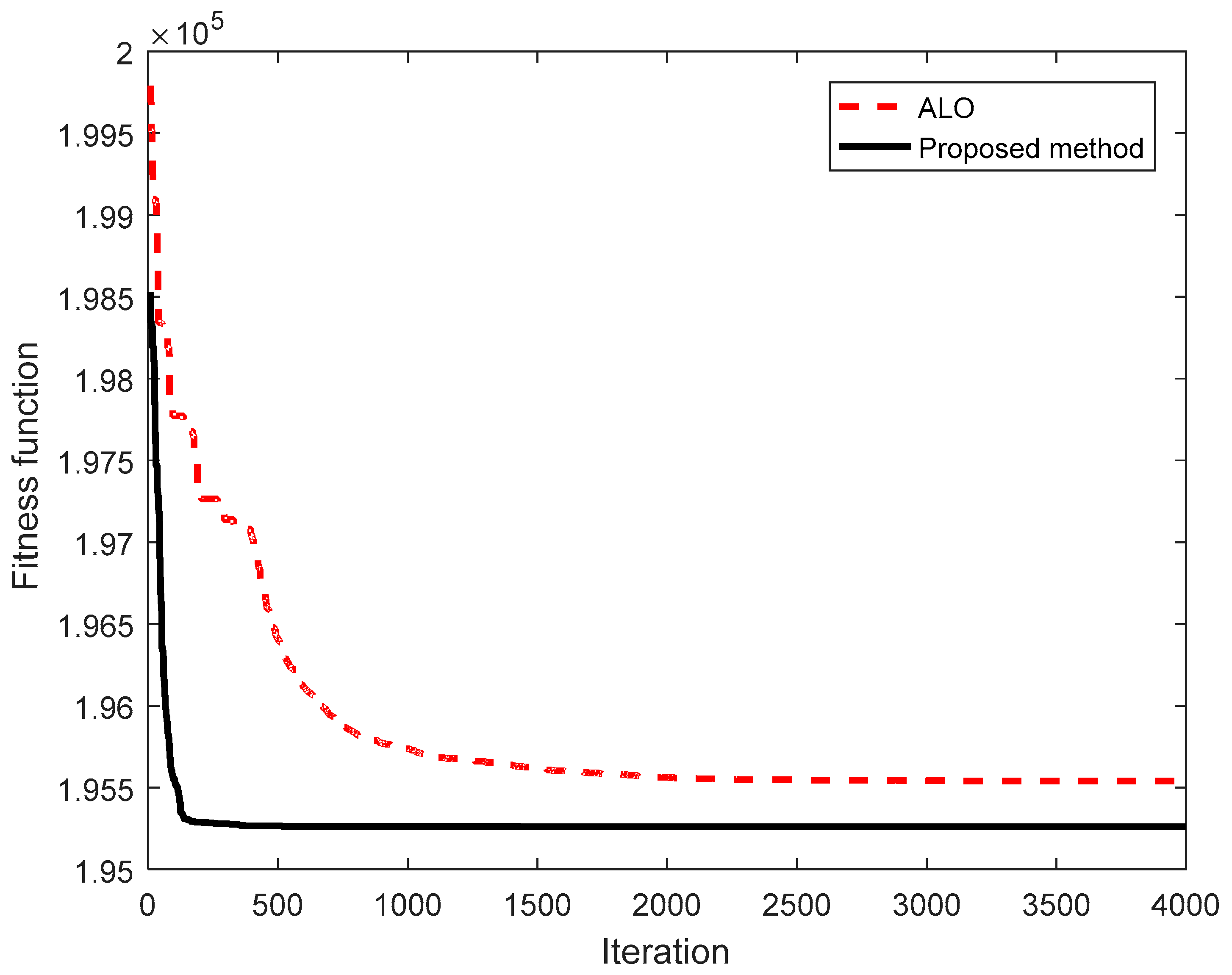
Figure 4,
Figure 5 and
Figure 6 indicate that the IALO was at least three times faster than the ALO, and the best solution of the ALO was much worse that the solution of the IALO at one third the number of iterations.
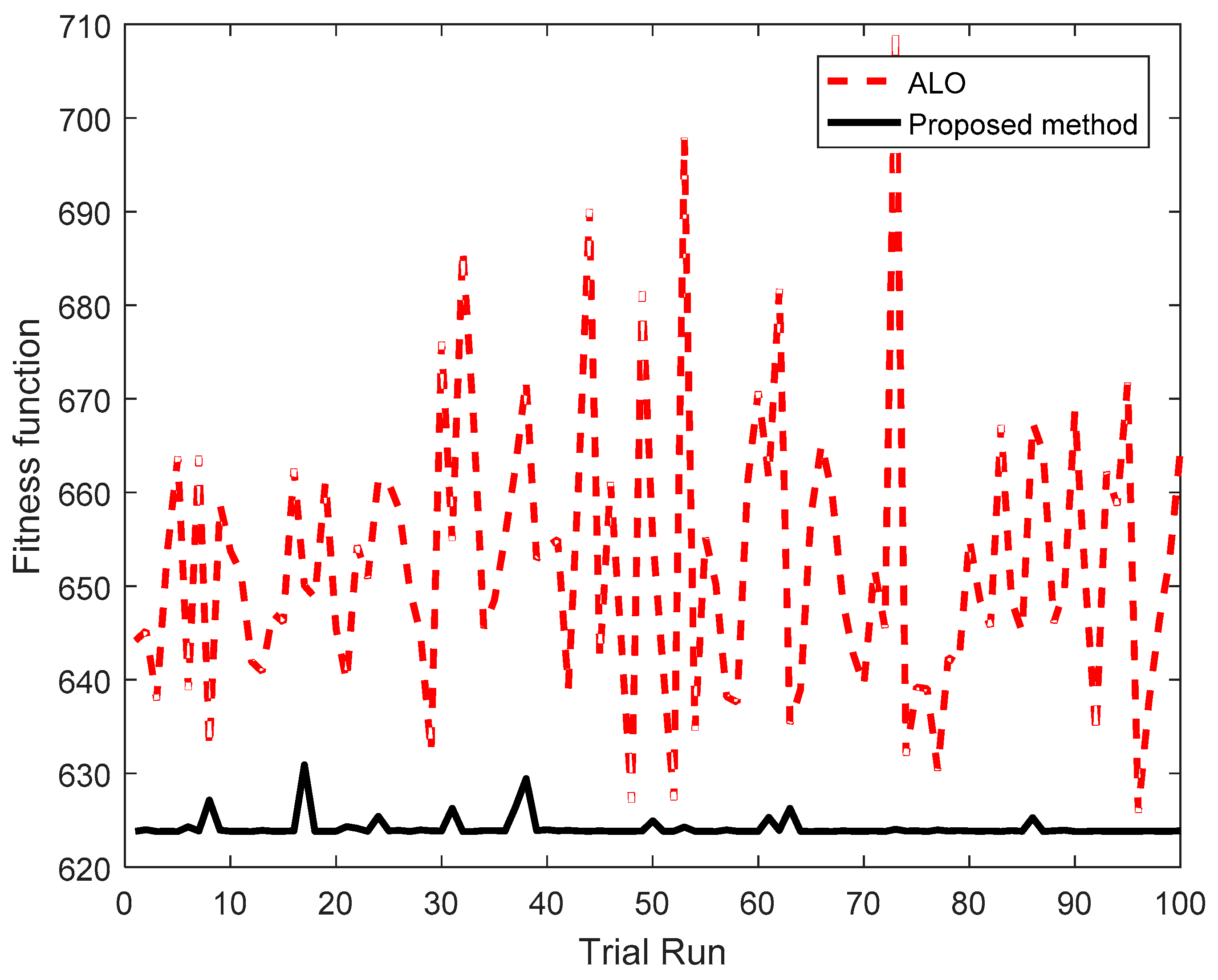
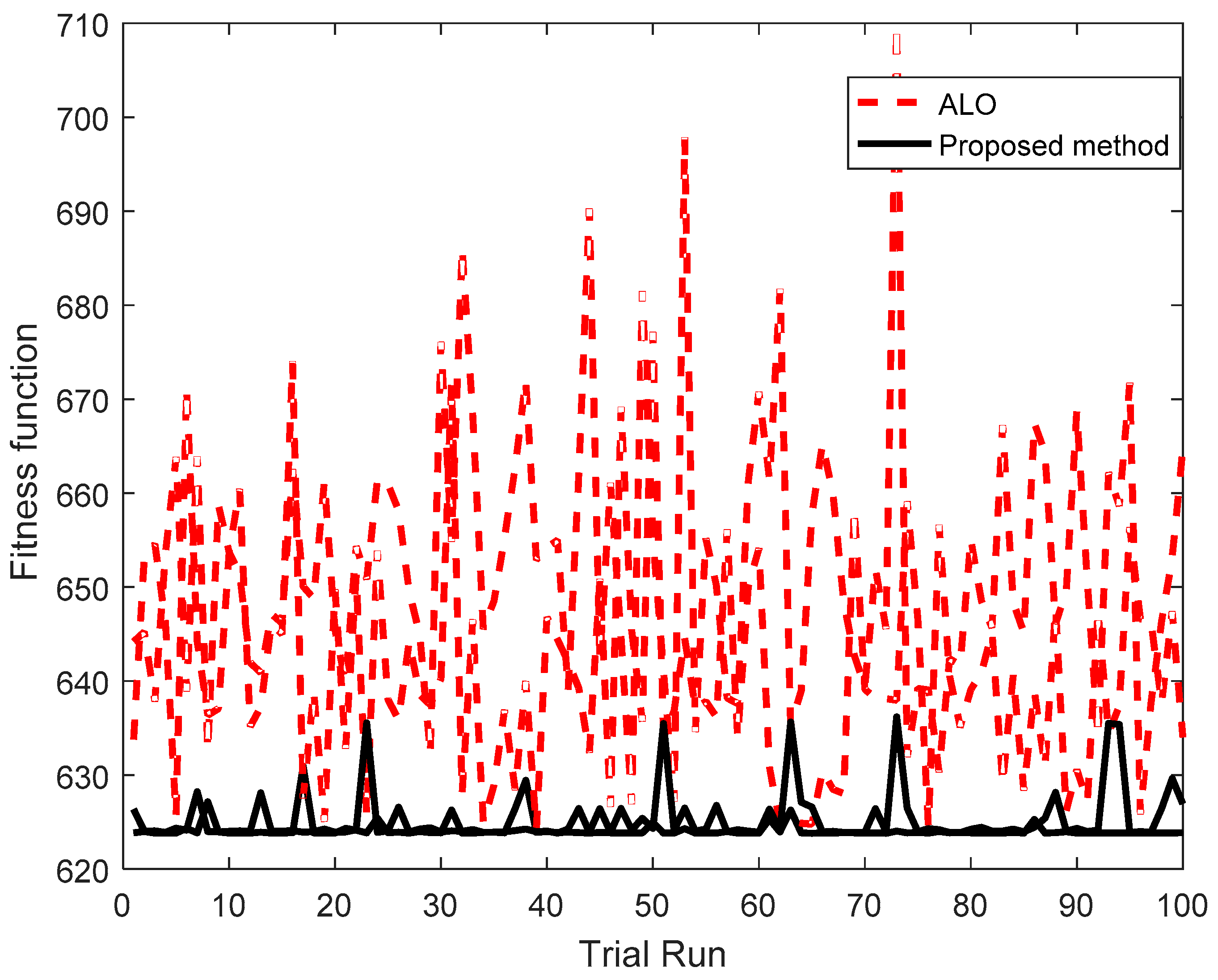
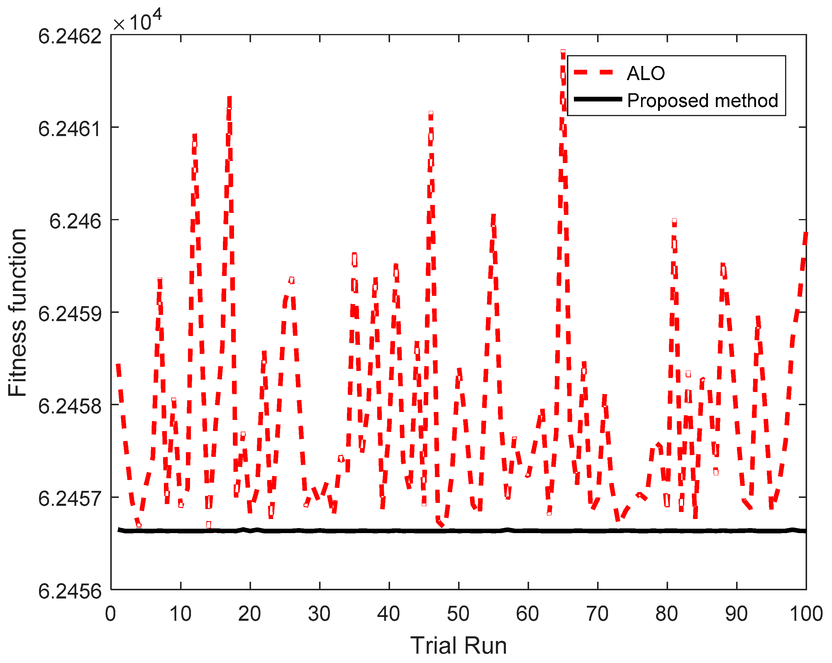
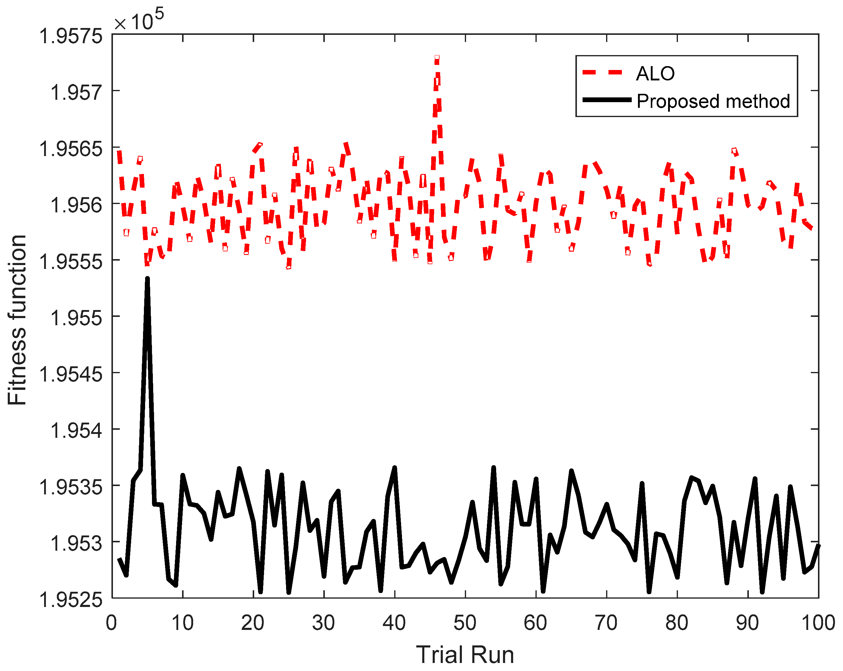
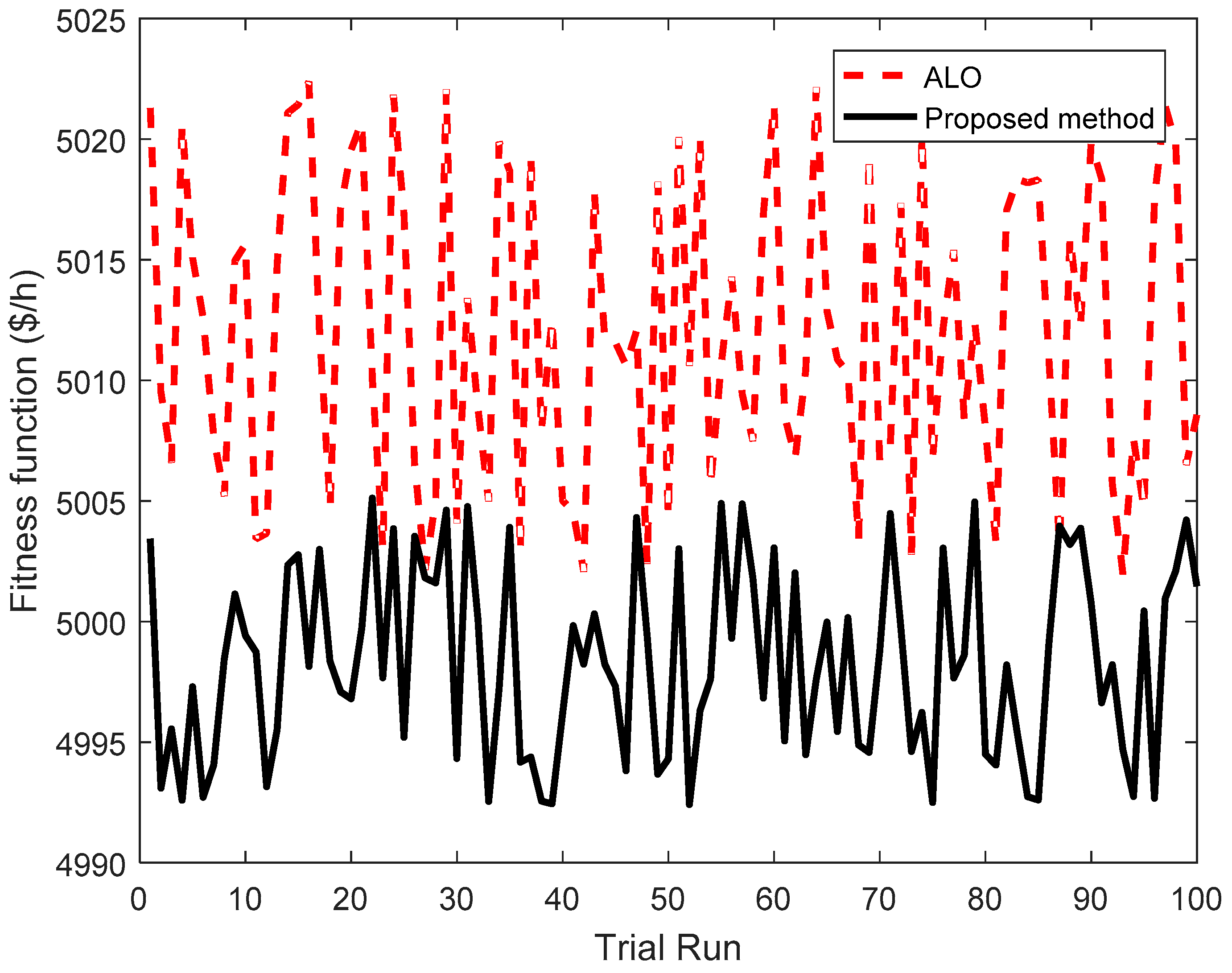
In order to investigate the efficiency of finding optimal solutions, the fitness of the best solution of successful runs was also plotted in
Figure 7,
Figure 8,
Figure 9,
Figure 10 and
Figure 11 for comparison. Fitness values of the IALO are black points while those of the ALO are red points. All the figures have the same characteristic that red points have very large fluctuations, but black points have very tiny deviations, even though they are on a line with the same fitness value. This manner implies that approximately all runs of the IALO are close to the best solution, but the ALO fails to reach the same achievement. Consequently, the performance improvement of the suggested IALO over the ALO is significant when dealing with these considered study cases.
Optimal generations of the studied cases found by the IALO are reported in
Appendix A.

 ,
, 


