Phase Equalization, Charge Transfer, Information Flows and Electron Communications in Donor–Acceptor Systems

Department of Theoretical Chemistry, Jagiellonian University, Gronostajowa 2, 30-387 Cracow, Poland
Appl. Sci. 2020, 10(10), 3615; https://doi.org/10.3390/app10103615
Submission received: 14 March 2020
/
Revised: 17 April 2020
/
Accepted: 23 April 2020
/
Published: 23 May 2020
(This article belongs to the Special Issue The Application of Quantum Mechanics in Reactivity of Molecules)
Abstract
:Subsystem phases and electronic flows involving the acidic and basic sites of the donor (B) and acceptor (A) substrates of chemical reactions are revisited. The emphasis is placed upon the phase–current relations, a coherence of elementary probability flows in the preferred reaction complex, and on phase-equalization in the equilibrium state of the whole reactive system. The overall and partial charge-transfer (CT) phenomena in alternative coordinations are qualitatively examined and electronic communications in A—B systems are discussed. The internal polarization (P) of reactants is examined, patterns of average electronic flows are explored, and energy changes associated with P/CT displacements are identified using the chemical potential and hardness descriptors of reactants and their active sites. The nonclassical (phase/current) contributions to resultant gradient information are investigated and the preferred current-coherence in such donor–acceptor systems is predicted. It is manifested by the equalization of equilibrium local phases in the entangled subsystems.
1. Introduction
The Information Theory (IT) [1,2,3,4,5,6,7,8] of Fisher [1] and Shannon [3] has been successfully applied in an entropic interpretation of the molecular electronic structure (e.g., [9,10,11]). Several information principles have been investigated [9,10,11,12,13,14,15,16] and pieces of molecular electron density attributed to Atoms-in-Molecules (AIM) have been approached [12,16,17,18,19,20], providing the IT basis for the intuitive stockholder division of Hirshfeld [21]. Patterns of entropic bond multiplicities have been extracted from electronic communications in molecules [9,10,11,22,23,24,25,26,27,28,29,30,31,32], information distributions in molecules have been explored [9,10,11,33,34], and the nonadditive Fisher (gradient) information [1,2,9,10,11,35,36] has been linked to Electron Localization Function (ELF) [37,38,39] of Density Functional Theory (DFT) [40,41,42,43,44,45]. This analysis has enabled a formulation of the novel Contragradience (CG) probe for localizing chemical bonds [9,10,11,46], while the Orbital Communication Theory (OCT) of the chemical bond using the “cascade” propagations in molecular information systems has identified the bridge interactions between AIM [11,47,48,49,50,51,52], realized through orbital intermediates.
In molecular Quantum Mechanics (QM), the wavefunction phase or its gradient determining the effective velocity of probability density and its current give rise to nonclassical information/entropy supplements to classical measures of Fisher [1] and Shannon [3]. In resultant IT descriptors of electronic states, the information/entropy content in the probability (wavefunction modulus) distribution is combined with the relevant complement due to the current density (wavefunction phase) [53,54,55,56,57,58,59,60,61,62]. The overall gradient information is then proportional to the expectation value of the system kinetic energy of electrons. Such combined descriptors are also required in the phase distinction between the bonded (entangled) and nonbonded (disentangled) states of molecular subsystems, e.g., the substrate fragments of reactive systems [63,64,65]. This generalized treatment then allows one to interpret the variational principle for electronic energy as equivalent information rule, and to use the molecular virial theorem [66] in general reactivity considerations [67,68,69,70,71].
The extremum principles for the global and local (gradient) measures of the state resultant entropy have determined the phase-transformed (“equilibrium”) states of molecular fragments, identified by their local “thermodynamic” phases [53,54,55,56,57]. The minimum-energy principle of QM has also been interpreted as physically-equivalent variational rule for the resultant gradient information, proportional to the state average kinetic energy [67,68,69,70,71]. In the grand-ensemble framework, they both determine the same thermodynamic equilibrium in an externally-open molecular system. This equivalence parallels identical predictions resulting from the minimum-energy and maximum-entropy principles of ordinary thermodynamics [72].
Elsewhere [63,73,74], the potential use of the DFT construction by Harriman, Zumbach, and Maschke (HZM) [75,76], of wavefunctions yielding the prescribed electron distribution, in a description of reactive systems has been examined. In such density-constrained Slater determinants, the defining Equidensity Orbitals (EO), of the Macke/Gilbert [77,78] type, exhibit the same molecular probability density, with the orbital orthogonality being assured by the EO local phases alone. These orbital states define the constrained multicomponent system composed of the mutually-closed orbital units, with each subsystem being characterized by its own phase and separate chemical-potential descriptors. Their simultaneous opening onto a common electron reservoir, and hence also onto themselves, generates the externally- and mutually-open orbital system, in which the EO fragments are effectively “bonded” (entangled) [63]. They then exhibit a common (molecular) phase descriptor and equalize their chemical potentials at the global reservoir level. This (mixed) equilibrium state is determined by the density operator corresponding to thermodynamic (grand-ensemble) probabilities of EO related to their orbital energies and average electron occupations.
In the present analysis, we focus on the phase component of electronic wavefunctions and the related current descriptor of molecular states, with special emphasis on the donor–acceptor reactive systems [63,67,68,69,70,71]. We examine the reactant phases and electronic flows involving the substrate acidic and basic active sites. The mutual relations between the state phase and current descriptors is explored, the phase-equalization in the equilibrium state of the whole reactive system is conjectured, and a coherence of probability flows in the preferred reaction complex is established. The overall and partial charge-transfer (CT) phenomena in alternative coordinations of the acidic (A) and basic (B) reactants are investigated, the electronic communications in alternative A—B complexes are qualitatively examined, and nonclassical contributions to the resultant gradient information are introduced. We also tackle the (internal) polarization (P) of reactants, induced by the (external) CT displacements between both substrates, and patterns of the resultant electronic flows on their active sites are qualitatively explored. The energy changes associated with specific P/CT fluxes in A—B systems are estimated using the familiar descriptors of the Charge Sensitivity Analysis (CSA) [79,80,81,82,83,84,85]: the global or regional chemical-potential/electronegativity [86,87,88,89,90] and hardness/softness [91] or Fukui function [92] descriptors of reactants and their acidic and basic active sites. The preferred coordination of reactants in such donor–acceptor systems is shown to exhibit a substantial current-coherence, which is also manifested by the equalization of the equilibrium local phases in the entangled (bonded) subsystems [63].
2. Molecular States and Their Phases
In QM, the state Ψ(N) of N-electrons is represented by its representative vector in the abstract (Hilbert) space,
where M stands for its modulus (“length”),
and |D(N)〉 denotes the corresponding directional (“unit”) vector:
A variety of quantum states is exhausted by all admissible orientations of the unit vector |D(N)〉 [93]. Thus, for the unity-normalized state vectors, when M = 1, |Ψ(N)〉 ≡ |D(N)〉.
|Ψ(N)〉 ≡ M|D(N)〉,
M = 〈Ψ(N)|Ψ(N)〉1/2 ≡ |Ψ(N)|,
|D(N)| = 〈D(N)|D(N)〉1/2 = 1.
The molecular state can be also identified by the spin-position representation of |Ψ(N)〉, called the wavefunction:
The squared modulus component,
determines the normalized probability distribution of N electrons:
Here, PΨ(N) and PQ(N) stand for the state and basis-set projection operators, respectively, while ∫dQ(N) denotes the integrations over spatial positions {rk} and summations over spin variables {σk} of all N electrons. The state exponential factor F(N) involves the N-electron phase function Φ[Ψ(N)]} ≡ Φ(N), which generates the state current density.
Ψ[Q(N)] = 〈Q(N)|Ψ(N)〉 ≡ Ψ(N) = D[Ψ(N)] exp{iΦ[Ψ(N)]} ≡ D(N) F(N).
D[Ψ(N)] = [Ψ(N)Ψ*(N)]1/2 ≡ D(N),
P(N) = D(N)2 = 〈Q(N)|Ψ(N)〉 〈Ψ(N)|Q(N)〉 ≡ 〈Q(N)|PΨ(N)|Q(N)〉
= 〈Ψ(N)|Q(N)〉 〈Q(N)|Ψ(N)〉 ≡ 〈Ψ(N)|PQ(N)|Ψ(N)〉,
= 〈Ψ(N)|Q(N)〉 〈Q(N)|Ψ(N)〉 ≡ 〈Ψ(N)|PQ(N)|Ψ(N)〉,
∫P(N) dQ(N) ≡ 1,
The wave function Ψ(N) thus reflects projections (directional “cosines”) of the state vector |Ψ(N)〉 onto the basis vectors {|Q(N)〉} of the adopted representation. It contains all essential “orientation” information about |Ψ(N)〉. This specific representation corresponds to the vector basis of N-electron states,
identified by the spin ({σk}) and position ({rk}) variables of all N electrons. It includes the eigenvectors {|qk〉} of the electronic spin (sk = isk,x + jsk,y + ksk,z, sk = −|sk|) and position (rk) operators:
|Q(N)〉 = |q1, q2, …, qN〉 = {|qk〉 = |σk, rk〉}, k = 1, 2, …, N,
sk2|qk〉 = ¾ ħ2|qk〉 ≡ sk2|qk〉, sk.z|qk〉 = σk ħ|qk〉 ≡ sz|qk〉, σk = ± ½, and
rk|qk〉 = rk|qk〉.
In what follows, we also examine (normalized) molecular orbital (MO) states {|ψw〉} of a single electron, |ψw| = 1. The state vector |ψw〉 is then given by the product of the spin (|ξw〉) and spatial (|φw〉) states:
It generates the associated spin-orbital (SO) function in q-representation,
the product of its normalized spin-function of an electron,
and the normalized (complex) spatial MO component,
with pw(r) = dw(r)2 defining the MO probability distribution. One customarily requires the spin-orbitals defining the N-electron configuration in a molecule to form the independent (orthonormal) set:
|ψw〉 ≡ |ξw〉|φw〉.
ψw(q) = 〈q|ψw〉 = 〈σ|ξw〉 〈r|φw〉 ≡ ξw(σ) φw(r),
ξw(σ) = 〈σ|ξw〉, |ξw| = (Σσ |ξw(σ)|2)1/2 = 1,
ξw(σ) ∈ {α(σ), spin-up; β(σ), spin-down},
φw(r) = 〈r|φw〉 = dw(r) exp[iϕw(r)] ≡ dw(r) fw(r),
∫φw(r)*φw(r) dr = 1 or |φw| = 1,
〈φv|φw〉 = ∫〈φv|r〉〈r|φw〉 dr = ∫φv(r)*φw(r) dr = δk,l.
To summarize, the complex MO wavefunction φw(r) fully reflects the orientation properties of |φw〉 in the position representation. The square of its modulus dw(r) = |φw(r)| determines the (normalized) spatial probability distribution in |ψw〉,
while |ξw(σ)|2 similarly determines the probability density of observing the specified spin component sz = σ ħ. The phase factor fw(r) = exp[iϕw(r)] identifies the orientation of the (normalized) state vector |φw〉 in the complex plane. It constitutes the r-representation of the directional (unit) vector
The MO phase gradient ultimately determines the orbital current
As an illustration, we summarize in Appendix A the components of the quantum state describing a single electron, explore its probability/current descriptors, and summarize the relevant continuity relations. The latter result directly from the Schrödinger equation (SE) of molecular QM (see Appendix B).
pw(r) = |φw(r)|2 = dw(r)2 ≥ 0, ∫pw(r) dr = 1,
|dw〉 = |φw〉/|φw| = |φw〉, |φw| = [∫|φw(r)|2 dr]1/2 ≡ 1,
dw(r) = 〈r|dw〉 = exp[iϕw(r)] = cosϕw(r) + i sinϕw(r).
jw(r) = [ħ/(2mi)] [φw(r)* ∇φw(r) − φw(r) ∇φw(r)*] = (ħ/m)] pw(r) ∇ϕw(r).
One finally recalls that in the one-electron (MO) approximation the N-electron wavefunctions are defined as Slater determinants constructed from the configuration occupied SO, ψ = (ψ1, ψ2, …, ψN),
Ψ(N) = 〈Q(N)|Ψ〉 = (N!)−1/2 |ψ1(Ψ)ψ2(Ψ) … ψN(Ψ)| ≡ det[ψ(Ψ)].
3. Electronic Communications
In OCT of the chemical bond [9,10,11,22,23,24,25,26,27,28,29,30,31,32,62], one explores the entropy/information descriptors of molecular information channels, e.g., the electron probability networks in the orthonormal Atomic Orbital (AO) resolution |χ〉 = {|χj〉, j = 1, 2, …, t},
Such electron communications are reflected by the conditional probabilities of observing in the molecular bond system the monitored “output” orbitals, given the specified “input” orbitals.
〈χi|χj〉 = ∫〈χi|r〉 〈r|χj〉 dr = ∫χi(r)* χj(r) dr = δi,j.
In this standard LCAO MO approach, the optimum MO |φ〉 = {|φw〉, w = 1, 2, …, t} are represented as Linear Combinations of the AO basis functions:
where the square matrix of the expansion coefficients, C = 〈χ|φ〉 = {Ci,w}, satisfies the matrix orthonormality relations:
The AO-resolved communication theory explores the entropy/information descriptors of the electronic-signal propagation network between “input” and “output” AO states.
φ(r) = {φw(r) = Σj χj(r) Cj,w} = χ(r) C, χ(r) = 〈r|χ〉,
CC† = {δi,j} = C†C = {δw,w’} ≡ I.
These scattering connections in the given electron configuration of Equation (20) are determined by its occupied MO, ψ(Ψ). The representative probability of observing in Ψ the specified output AO χj(r) = 〈r|χj〉 = mj(r) exp[iϕj(r)], given the input AO χi(r) = 〈r|χi〉= mi(r) exp[iϕi(r)],
is generated by the squared modulus of the associated conditional amplitude A(χj|χi) ≡ A(j|i):
Here, P(χi) ≡ P(i) denotes the probability of detecting AO state |χi〉 ≡ |i〉 in the chemical bond system of the electron configuration in question, while P(χi, χj) ≡ P(i, j) stands for the joint-probability of these two AO events, of simultaneously observing the two AO states |i〉 and |j〉 in Ψ. These probabilities satisfy the relevant normalizations:
P(χj|χi) = P(χi, χj)/P(χi) ≡ P(j|i), Σj P(j|i) = 1,
{P(j|i) ≡ |A(j|i)|2}.
Σi [Σj P(i, j)] = Σi P(i) = 1.
In accordance with the Superposition Principle (SP) of QM [93], the scattering amplitude A(ζ|θ) between states θ(r) ≡ 〈r|θ〉 = mθ(r) exp[iϕθ(r)] and ζ(r) ≡ 〈r|ζ〉 = mζ(r) exp[iϕζ(r)] is defined by the mutual projection of the two state-vectors involved:
This conditional amplitude is thus generated by the (local) effective modulus function M(ζ|θ) = mθ(r) mζ(r) and the phase component
Therefore, the conditional probability P(θ|ζ) can be interpreted as the expectation value in one state of the (idempotent) projection operator onto another state:
A(ζ|θ) = 〈θ|ζ〉 ≡ ∫θ(r)* ζ(r) dr = ∫mθ(r) mζ(r) exp{i[ϕζ(r)−ϕθ(r)]} dr
≡ ∫M(ζ|θ) exp{iΦ(ζ|θ)] dr.
≡ ∫M(ζ|θ) exp{iΦ(ζ|θ)] dr.
Φ(ζ|θ) = ϕζ(r) − ϕθ(r).
P(θ|ζ) ≡ |A(θ|ζ)|2 = 〈ζ|θ〉 〈θ|ζ〉 ≡ 〈ζ|Pθ|ζ〉
= 〈θ|ζ〉 〈ζ|θ〉 ≡ 〈θ|Pζ|θ〉,
Pϑ = |ϑ〉 〈ϑ|, Pϑ2 = Pϑ, ϑ = (θ, ζ).
= 〈θ|ζ〉 〈ζ|θ〉 ≡ 〈θ|Pζ|θ〉,
Pϑ = |ϑ〉 〈ϑ|, Pϑ2 = Pϑ, ϑ = (θ, ζ).
In molecular electron configuration of Equation (20), each AO event is additionally conditional on the molecular state Ψ(N), identified either by the N-electron projection operator PΨ(N) = |Ψ(N)〉〈Ψ(N)| or the configuration (idempotent) bond-projection Pb(N) involving only the occupied MO selected by their finite occupation numbers
where w = 1, 2, …, t (all SO, occupied, and virtual) and s = 1, 2, …, N (occupied SO only).
n(Ψ) = {nw(Ψ)δw,w’},
nw(Ψ) = 1 (Ψ-occupied MO) or nw(Ψ) = 0 (Ψ-virtual MO),
Pb(Ψ) = |Ψ(Ψ)〉 n(Ψ) 〈Ψ(Ψ)| = Σw |ψw(Ψ)〉 nw(Ψ) 〈ψw(Ψ)|
= Σs |Ψs(Ψ)〉 〈Ψs(Ψ)| ≡ Σs Ps(Ψ),
= Σs |Ψs(Ψ)〉 〈Ψs(Ψ)| ≡ Σs Ps(Ψ),
The conditional probability of observing |j〉 given |i〉 in electronic configuration |Ψ〉 thus involves the doubly-conditional (coherent) amplitude AΨ(χj|χi) ≡ A(χj|χi‖Ψ) ≡ AΨ(j|i):
Its amplitude
thus defines the relevant element of the (idempotent) Charge-and-Bond−Order (CBO) matrix of LCAO MO theory:
This molecular communication amplitude is thus characterized by the effective modulus and phase components of γi,j(Ψ) resulting from corresponding descriptors of (complex) LCAO MO coefficients
PΨ(χj|χi) = P(χj|χi‖Ψ) ≡ PΨ(j|i) = |AΨ(j|i)|2.
AΨ(j|i) = 〈i|Pb(Ψ)|j〉 = Σw 〈i|ψw(Ψ)〉 nw(Ψ) 〈ψw(Ψ)|j〉
= Σs 〈i|Ψs(Ψ)〉 〈Ψs(Ψ)|j〉 = Σs Ci,s(Ψ) Cj,s(Ψ)*≡ γi,j(Ψ)
= Σs 〈i|Ψs(Ψ)〉 〈Ψs(Ψ)|j〉 = Σs Ci,s(Ψ) Cj,s(Ψ)*≡ γi,j(Ψ)
γ(Ψ) = 〈χ|Ψ(Ψ)〉 n(Ψ) 〈Ψ(Ψ)|χ〉 = C(Ψ) n(Ψ) C(Ψ)† = {γi,j(Ψ)}.
C(Ψ) = {Ck,w(Ψ) = 〈χk|ψw(Ψ)〉 ≡ 〈k|ψw(Ψ)〉.
For the given electron configuration |Ψ(N)〉, it determines the molecular conditional probabilities between the specified pair of AO states. These scattering probabilities are now defined by the AO expectation values of the (nonidempotent) basis set projections in the occupied MO subspace,
of the system chemical bonds in |Ψ(N)〉:
Plb(Ψ) = Pb(Ψ) |l〉 〈l| Pb(Ψ) = Pb(Ψ) Pl Pb(Ψ), [Plb(Ψ)]2 ≠ Plb(Ψ),
PΨ(j|i) ≡ |AΨ(j|i)|2 = γi,j(Ψ) γj,i(Ψ)
= 〈i|Pb(Ψ)|j〉 〈j|Pb(Ψ)|i〉 = 〈i|Pb(Ψ)PjPb(Ψ)|i〉 ≡ 〈i|Pjb(Ψ)|i〉
= 〈j|Pb(Ψ)|i〉 〈i|Pb(Ψ)|j〉 = 〈j|Pb(Ψ)PiPb(Ψ)|j〉 ≡ 〈j|Pib(Ψ)|j〉.
= 〈i|Pb(Ψ)|j〉 〈j|Pb(Ψ)|i〉 = 〈i|Pb(Ψ)PjPb(Ψ)|i〉 ≡ 〈i|Pjb(Ψ)|i〉
= 〈j|Pb(Ψ)|i〉 〈i|Pb(Ψ)|j〉 = 〈j|Pb(Ψ)PiPb(Ψ)|j〉 ≡ 〈j|Pib(Ψ)|j〉.
4. Phase–Current Relation
In this section, we briefly explore the mutual relation between the phase and current descriptors [see Equation (19)] of the quantum state of an electron,
where
Its probability distribution reflects the square of the MO modulus factor, p(r) = m(r)2, while its phase component ϕ(r) determines the state probability current of Equation (19):
Here, the effective velocity of the probability “fluid”,
measures the local current-per-particle and reflects the state phase gradient:
ψ(q) = φ(r)ξ(σ),
φ(r) = m(r) exp[iϕ(r)].
j(r) = [ħ/(2mi)] [φ(r)* ∇φ(r) − φ(r) ∇φ(r)*]
= (ħ/m) p(r) ∇ϕ(r) ≡ p(r) V(r).
= (ħ/m) p(r) ∇ϕ(r) ≡ p(r) V(r).
V(r) = {Vu(r) ≡ Vu(u, {v≠u}), u = x, y, z},
V(r) = j(r)/p(r) = (ħ/m) ∇ϕ(r).
Therefore, velocity components of the probability flux are determined by the corresponding partials of the state phase function:
It follows from this equation that the phase of electronic state can be formally reconstructed by an indefinite integration of the corresponding components of the velocity field of the probability flux:
Vu(r) = (ħ/m) [∂ϕ(r)/∂u], u = x, y, z.
As an illustrative example, consider the fixed-momentum (free-particle) state
One indeed recovers its phase components,
by straightforward unidimensional integrations of Equation (40).
φK(r) = A exp(iK·r) = A exp[i(Kxx + Kyy + Kzz),
K = (m/ħ)V, V = iVx + jVy + kVz = const.
ϕ(r) = K·r = (m/ħ) (Vxx + Vyy + Vzz),
Consider now the phase/current dependent term of the overall content of MO resultant gradient-information [28,53,54,55,56,57,58,59,60,61,62] in Quantum Information Theory (QIT) [62]:
By analogy to the free-electron wavefunction of Equation (41), one introduces the wave-vector distribution in molecular systems, defined by the local phase gradient
In terms of this local momentum measure, the nonclassical information functional simplifies:
I[ϕ] = 4∫p(r) [∇ϕ(r)]2dr ≡ ∫p(r) Iϕ(r) dr
= (2m/ħ)2 ∫p(r) V(r)2 dr = (2m/ħ)2 ∫p(r)−1 j(r)2 dr.
= (2m/ħ)2 ∫p(r) V(r)2 dr = (2m/ħ)2 ∫p(r)−1 j(r)2 dr.
K(r) = (m/ħ) V(r) = ∇ϕ(r).
I[ϕ] = 4 ∫p(r) K(r)2dr ≡ 4〈K2〉.
Therefore, in such an inhomogeneous (molecular) electron density, the nonclassical MO information reflects the state average square 〈K2〉 of the wave-vector K(r). It thus follows from the preceding equation that this nonclassical information measure, related to the current contribution to the state resultant kinetic energy, depends only on the magnitude of the local probability flow, being independent of its direction.
5. Current Coherence in Donor–Acceptor Systems
Electron flows in molecules are determined by the energy conditions. The molecular energetics is reflected by SE of QM. Indeed, the entropy/information flows in molecular systems are carried by the state electronic flows. The QIT description thus offers only a supplementary, alternative framework for exploring and ultimately better understanding the rules and structures of chemistry. The energetics of a nondegenerate ground-state of the whole molecular system is devoid of any phase aspect, while subtle preferences involving reactants may already involve local phases of electronic states in the substrate subsystems, reflecting their entanglement in the whole reactive complex [63,64,65,66,67,68,69,70,71].
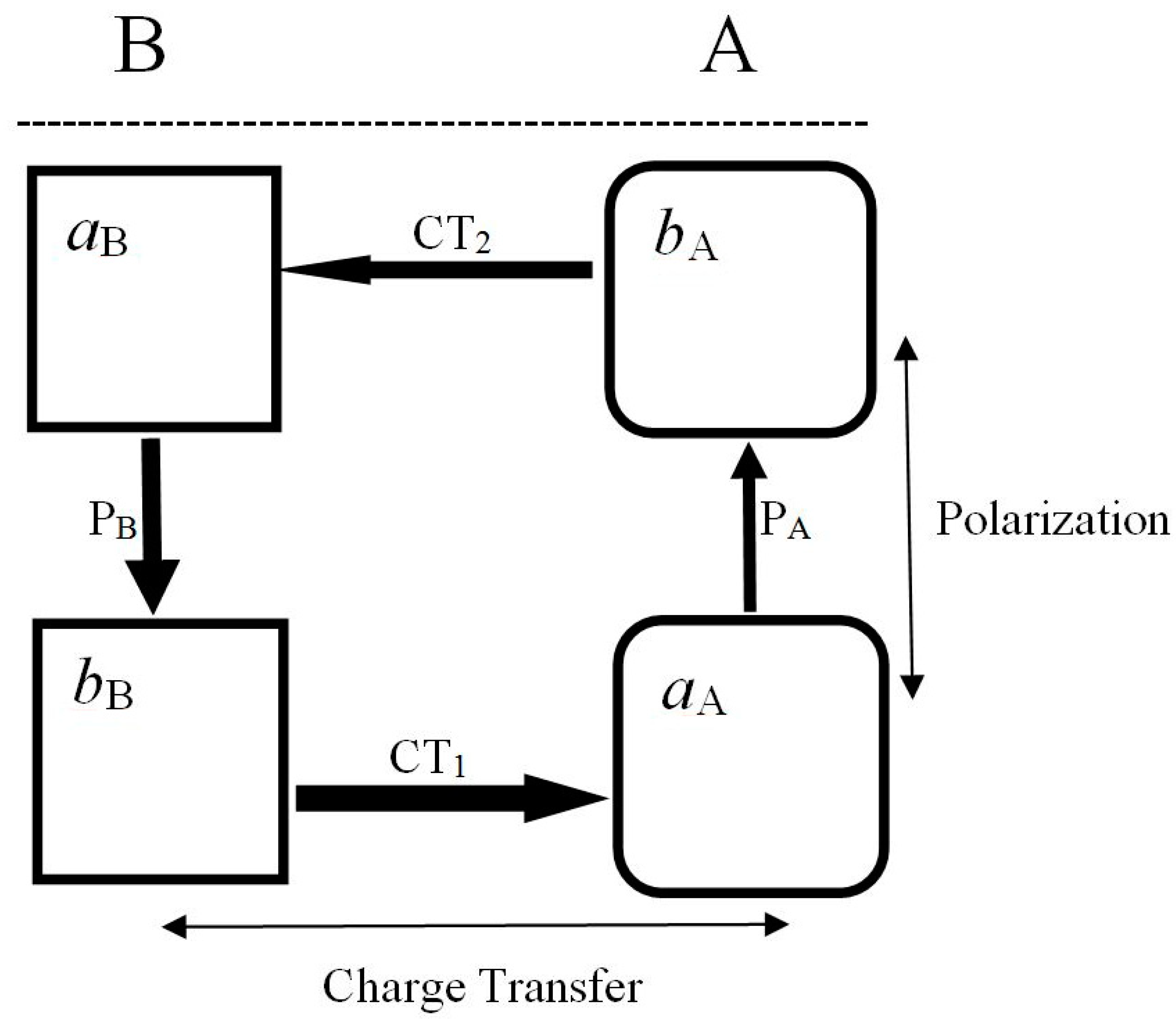
As an illustrative example let us now recall the energy-preferred complementary reactive complex A—B [67,70,94,95] shown in Figure 1, consisting of the basic subsystem
and its reaction companion—the acidic substrate
where aX and bX denote the active acidic and basic sites of X, respectively. The four molecular fragments, λ ∈{(aA, bA), (aB, bB)}, define the active parts in the system charge reconstruction. The acidic (electron acceptor) part is relatively harder, i.e., less responsive to external perturbations, thus exhibiting lower values of the fragment Fukui function or chemical softness descriptor, while the basic (electron donor) fragment is relatively more polarizable, as indeed reflected by higher response descriptors of its electron density or site populations. The acidic part aX exerts an electron-accepting (stabilizing) influence on the neighboring part of another reactant Y, while the basic fragment bX produces an electron-donor (destabilizing) effect on the fragment Y in its vicinity.
B = (aB |…| bB) ≡ (aB|bB)
A = (aA |…| bA) ≡ (aA|bA),
In the most stable complementary (c) complex of Figure 1 [94,95], a geometrically accessible a-fragment of one reactant faces the geometrically accessible b-fragment of the other substrate
while in a less favorable regional HSAB-type coordination the acidic (basic) fragment of one reactant faces the like-fragment of the other substrate:
A relative stability of Rc reflects an electrostatic preference: an electron-rich (repulsive, basic) fragment of one reactant indeed prefers to face an electron-deficient (attractive, acidic) part of the reaction partner. As shown in Figure 1, at finite separations between the two subsystems, spontaneous (primary) CT displacements between reactants trigger the induced (secondary) polarizational flows {PX} within each reactant, which restore the intra-substrate equilibria initially displaced by the presence of the other fragment and the inter-reactant CT:
It has been inferred from the (energetic) Electronegativity Equalization principle [95] that the electronic CT and P flows in Rc generate the concerted pattern shown in Figure 1 and Equation (48), which exhibits the maximum current (phase-gradient) coherence. It implies the least population activation on both reactants, which also energetically favors the complementary complex relative to the regional HSAB arrangement. Indeed, in RHSAB coordination the energy-preferred disconcerted flow pattern implies a more exaggerated depletion of electrons on bB and their more accentuated accumulation on aA. In fact, these partial flows of electrons signify the “bridge” CT between the key (“diagonal”) sites bB and aA, via the intermediate (“off-diagonal”) sites aB and bA.
In the complementary arrangement of both reactants, the partial fluxes involving the four active sites indicate the “flow-through” behavior of all these fragments, which combines the external (CT) and internal (P) currents. One observes that the acidic sites accept electrons as a result of charge transfer between reactants and donate electrons through the substrate polarization. The opposite behavior of the basic sites is observed: they receive electrons due to P-mechanism and lose electrons as a result of CT. In the HSAB complex, one observes a similar flow-through pattern only on the aB and bA sites, bB exclusively donates electrons both internally (P) and externally (CT), while aA only accepts electrons from its complementary fragment bA (P) and aB (CT) part of the other reactant.
To summarize, in Rc, one observes the concerted flow of electrons involving all four active sites of both reactants, with small net changes in electron populations on these fragments, while the charge reconstruction in RHSAB can be regarded as a transfer of electrons from bB to aA through the remaining (intermediate) sites aB and bA. The energetical preference of the complementary arrangement of reactants [94,95] also signifies the maximum phase-gradient coherence on each site, with its P or CT inflow part being accompanied by the associated outflow flux. Such a flow pattern thus corresponds to the least populational displacements on all constituent active sites. The above “activation” perspective then provides a natural physical explanation of the observed preference of the complementary coordination.
The energetically favored, concerted pattern of electronic fluxes in Rc can be realized only by an appropriate coherence of the site effective phase-gradients, of the pure or mixed states {Ψλ} describing the mutually-closed fragments λ ∈ {aA =1, bA = 2, aB = 3, bB = 4} of both reactants. These states define the average resultant currents on each site, weighted by the site electron probability distribution pλ(r),
already accounting for the average outflows-from and inflows-to the part in question, caused by the CT or P displacements in the system electronic structure.
〈j〉λ = ∫pλ(r) jλ(r) dr ≡ j(λ), ∫pλ(r) dr = 1,
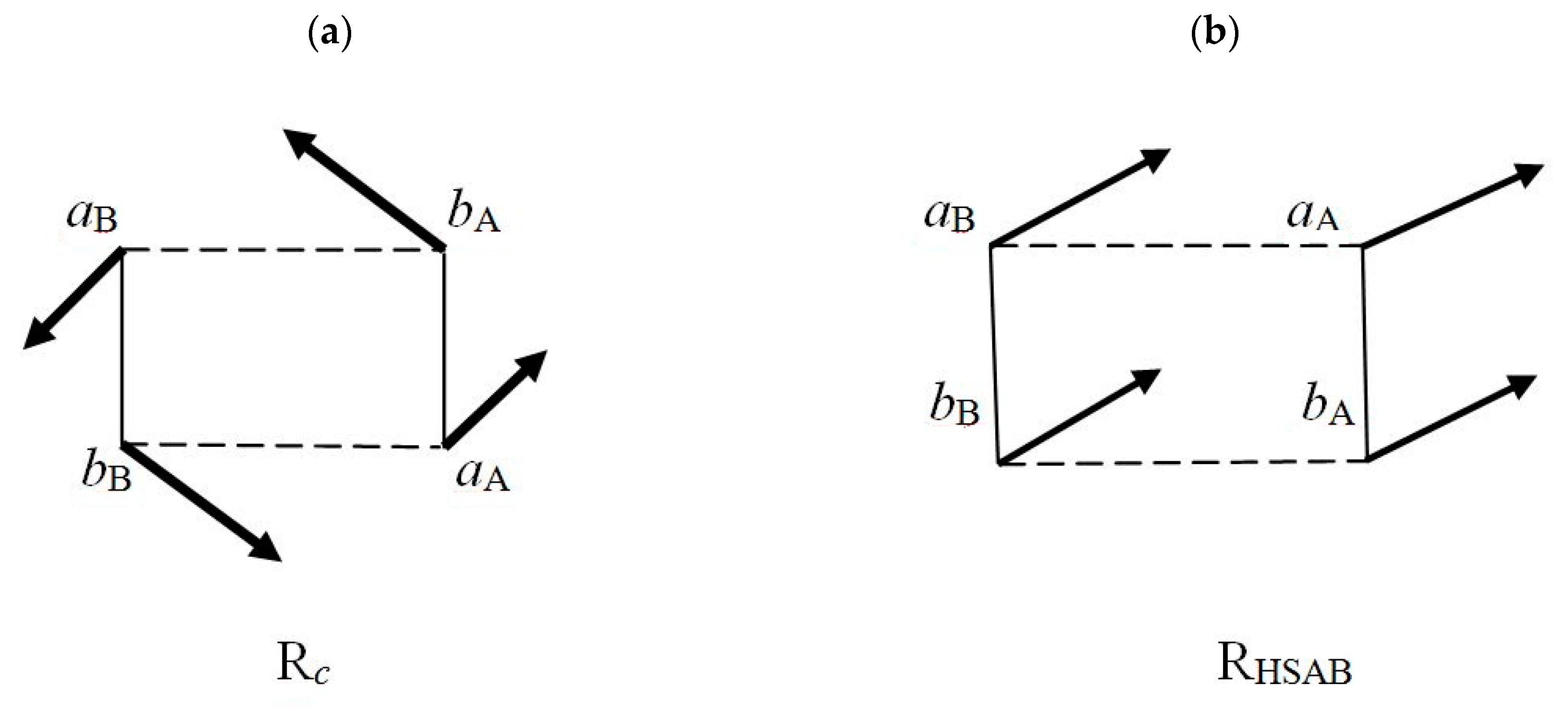
The elementary P and CT currents of the flow-patterns in Equation (48) give rise to the corresponding vector sums {j(λ)}, the site resultant currents schematically drawn in Figure 2. They are seen to generate a “conrotatory” pattern in the complementary complex Rc and a collective “translational” pattern in RHSAB. The magnitude |〈j〉λ| of this average (directional) site descriptor of the probability-flow ultimately determines the size |ΔNλ| of the net change in the fragment electron population in unit time,
where Nλ stands for the fragment average number of electrons in the separate reactant. The energy-favored (complementary) complex, which represents the least population-activation process, then corresponds to the lowest overall population displacement:
ΔNλ = Nλ 〈j〉λ,
Σλ |ΔNλ| = Σλ Nλ |〈j〉λ| ≡ Σλ Nλ 〈j〉λ ⇒ minimum.
A reference to Equation (43) shows that the nonclassical gradient information of site λ also probes the average lengths of the directional phase-related properties:
Therefore, the least site-activation of Equation (51), which occurs for the current-coherence in reactive system, also implies the minimum of the (additive) overall nonclassical information content:
Its absolute minimum is reached for the mutually-open (entangled) sites in the (bound) nondegenerate quantum state of the whole reactive system,
when the local phase contribution identically vanishes. Moreover, in the information equilibrium state of the entangled molecular fragments, corresponding to the minimum of the system nonclassical gradient-information, this also implies the equalization of subsystem phases at the global phase of the wavefunction describing the reactive system as a whole (see also Appendix C).
Iλ[ϕλ] = 4∫pλ(r) [∇ϕλ(r)]2dr
= (2m/ħ)2 ∫pλ(r) Vλ(r)2 dr
= (2m/ħ)2 ∫pλ(r)−1 jλ(r)2 dr.
= (2m/ħ)2 ∫pλ(r) Vλ(r)2 dr
= (2m/ħ)2 ∫pλ(r)−1 jλ(r)2 dr.
I[ϕ] = Σλ Iλ[ϕλ] ⇒ minimum.
R* = (A* ¦ B*) = (aA* ¦ bA* ¦ aB* ¦ bB*),
The normalized probability distributions on sites {κ = (a, b)} in reactants {X = (A, B)},
the shape factors of the fragment electronic densities {ρκ(r; X)}, can be used as weights in determining the corresponding fragment (internal) averages of physical properties. For example, the site vector (directional) densities
generate the associated average descriptors on each substrate:
Here, N(X) = Σκ Nκ(X) stands for the global number of electrons in reactant X,
denotes the site probability in X, and the fragment and local weighting factors obey the usual (internal) normalizations for each reactant:
{pλ(r)} = {pκ(r; X) = ρκ(r; X)/Nκ(X)}, ∫pκ(r; X) dr = 1,
{kκ(r; X)}, {Vκ(r; X)} and {jκ(r; X)}
〈k(X)〉 = Σκ Pκ(X) ∫pκ(r; X) kκ(r; X) dr ≡ Σκ Pκ(X) 〈k(X)〉κ
≡ Σκ ∫wκ(r; X) kκ(r; X) dr ≡ ∫k(r; X) dr,
≡ Σκ ∫wκ(r; X) kκ(r; X) dr ≡ ∫k(r; X) dr,
〈V(X)〉 = Σκ Pκ(X) ∫pκ(r; X) Vκ(r; X) dr ≡ Σκ Pκ(X) 〈V(X)〉κ
≡ Σκ ∫wκ(r; X) Vκ(r; X) dr ≡ ∫V(r; X) dr,
≡ Σκ ∫wκ(r; X) Vκ(r; X) dr ≡ ∫V(r; X) dr,
〈j(X)〉 = Σκ Pκ(X) ∫pκ(r; X) jκ(r; X) dr ≡ Σκ Pκ(X) 〈j(X)〉κ
≡ Σκ ∫wκ(r) jκ(r; X) dr ≡ ∫j(r; X) dr.
≡ Σκ ∫wκ(r) jκ(r; X) dr ≡ ∫j(r; X) dr.
Pκ(X) = Nκ(X)/N(X)
Σκ Pκ(X) = Σκ ∫wκ(r; X) dr = 1.
The corresponding quantities in the whole reactive system then result from weighting these substrate averages with their probabilities in R as a whole:
{PX(R) = N(X)/N(R)}, N(R) = ΣX N(X);
〈k(R)〉 = ΣX PX(R) 〈k(X)〉, 〈V(R)〉 = ΣX PX(R) 〈V(X)〉, 〈j(R)〉 = ΣX PX(R) 〈j(X)〉.
6. Overall Charge Transfer
Let us now briefly examine some energetic consequences of such displacements in electron populations on these functional sites of the acidic and basic subsystems [79,80,81,82,83,84,85]. The known (external) CT action of these substrates in the reactive complex R, the net inflow of electrons to A and an outflow from B, suggests the use of the “biased” estimates of the chemical potentials of the equilibrium reactant subsystems
in the polarized reactive complex Rα+, α = (c, HSAB), defining its substrate-resolution. It combines the internally-open but mutually-closed reactants in presence of each other:
A+ = (aA+ ¦ bA+) and B+ = (aB+ ¦ bB+)
Rα+ = [A+(α)|B+(α)] = [aA+(α) ¦ bA+(α) | aB+(α) ¦ bB+(α)].
Each coordination α defines its specific external potential due to the fixed nuclei in both subsystems,
which is constrained in definitions of the substrate populational derivatives of Rα+: the reactant chemical potentials and hardness descriptors.
v(α) = vA(α) + vB(α),
The chemical potentials (negative electronegativities) of reactant subsystems in Rα+, μ(Rα+) = {μα(X+)}, represent partial derivatives of the system energy Eα+[N(Rα+)}, v(α)] with respect to the substrate electronic populations N(Rα+) = {Nα(X+)} for the fixed external potential v(α), i.e., the “frozen” geometry of the whole reactive system,
μα(X+) ≡ ∂Eα+[N(Rα), v(α)]/∂Nα(X+)]v(α), α = (c, HSAB), X+ ∈ (A+, B+).
These population “potentials” also reflect the subsystem electronegativities,
measuring the related partials of electronic energy Eα+[Q(Rα+), v(α)] with respect to the reactant net-charges Q(Rα+) = {Qα(X+)}, dQα(X+) = −dNα(X+).
χα(X+) ≡ ∂Eα+[Q(Rα+), v(α)]/∂Qα(X+)]v(α) = −μα(X+),
The internally-equalized chemical potentials
of the basic and acidic reactants, when acting as donor (B) and acceptor (A) of electrons, respectively, then read:
where IX+ and AX+ denote the ionization potential and electron affinity of X+, respectively. These biased substrate descriptors apply to both Rc+ and RHSAB+ complexes. Indeed, in the complementary arrangement, the amount of the first partial charge transfer dominates the second one (see Figure 1), N(CT1) > N(CT2), so that B+ net donates and A+ accepts electrons.
μ(Rα+) = [∂Eα+/∂N(Rα+)] v(α) = {μα(X+) = ∂Eα+/∂Nα(X+)}
μα(A+) = μα(aA+) = μα(bA+) = −IA+ and
μα(B+) = μα(aB+) = μα(bB+) = −AB+,
μα(B+) = μα(aB+) = μα(bB+) = −AB+,
The optimum amount of the resultant CT between A+ and B+ substrates in Rα+,
where {Nα(X0)} denote electron numbers in separate reactants and {N(X*)} stand for the average electron populations in the coordination final, equilibrium reactive system with the mutually-open subsystems,
is determined by the corresponding in situ CT “force”, the effective chemical-potential for this process (populational “gradient”), measuring the difference between chemical potentials of the polarized acidic and basic reactants,
and the coordination in situ hardness descriptor η(CT) for this electron transfer,
representing the effective CT-hardness (populational “Hessian”). Here, the elements of the hardness tensor in reactant resolution measure the second populational partials
Since the acidic (basic) reactants are identified by their chemically hard (soft) character, as substrates of relatively small (high) polarizability, their chemical potentials obey the following inequality: μα(A+) < μα(B+) < 0.
Nα(CT) = Nα(A*) − Nα(A0) = Nα(B0) − Nα(B*) > 0,
Rα* = [A*(α) ¦ B*(α)] = [aA*(α) ¦ bA*(α) ¦ aB*(α) ¦ bB*(α)],
μα(CT) = ∂Eα+[Nα(CT), v(α)]/∂Nα(CT) = μα(A+) − μα(B+) < 0,
ηα(CT) = ∂μα(CT)/∂Nα(CT)
= ηα(A+,A+) − ηα(A+,B+) + ηα(B+,B+) − ηα(B+,A+) > 0,
= ηα(A+,A+) − ηα(A+,B+) + ηα(B+,B+) − ηα(B+,A+) > 0,
η(Rα+) = [∂2Eα+/∂N(Rα+) ∂N(Rα+)]v(α) = [∂μ(Rα+)/∂N(Rα+)]v(α) = {ηα(X+,Y+)},
ηα(X+,Y+) ≡ {∂2Eα+[{N(Rα+)}, v(α)]/∂Nα(X+) ∂Nα(Y+)}v(α)
= [∂μα(X+)/∂Nα(Y+)]v(α), X+, Y+ ∈ (A+, B+).
= [∂μα(X+)/∂Nα(Y+)]v(α), X+, Y+ ∈ (A+, B+).
Finally, the coordination equilibrium amount of the inter-reactant CT [79,80,82],
generates the associated 2nd-order stabilization energy due to CT,
Nα(CT) = −μα(CT)/ηα(CT),
Eα(CT) = μα(CT) Nα(CT)/2 = − [μα(CT)]2/[2ηα(CT)] < 0.
It should be emphasized that this energy estimate already contains the implicit polarization contributions, due to internal charge adjustments within each internally-open reactant. Indeed, all spontaneous electron flows, of both of CT and P origins, stabilize the system.
7. Partial Electronic Flows
It is also of interest to establish energy contributions due to all partial electronic flows shown in the flux patterns in Equation (48), of both P and CT origins. As observed above, all such spontaneous responses of the reactive system contribute the stabilizing (negative) contributions to the reaction energy. The P-currents represent the intra-reactant responses created by a presence of the other substrate and the external CT.
The P/CT resolved flow patterns in Equation (48) and the associated energy terms call for the site-resolution of the polarized reactive system, now corresponding to the mutually-closed reaction sites on the internally- and mutually-closed reactants A = (aA | bA) and B = (aB | bB) (see Figure 1), for the external potential v(α) of Equation (64),
Their functional fragments, the acidic and basic sites in both reactants,
which contain n(Rα) = {nλ(α)} electrons, are then characterized by different levels of the site chemical potentials
measured by the partial energy derivatives with respect to average electron populations:
The site-hardness descriptors are similarly defined by the corresponding matrix of the second populational derivatives of the energy in this resolution level:
In this more resolved perspective, one also applies the biased estimates of the fragment chemical potentials, measured either by the site negative ionization potential (uλ = −Iλ) or its negative electron affinity (uλ = −Aλ), when this fragment acts as an external electron donor or acceptor, respectively.
Rα = [A(α) | B(α)] = [aA(α) | bA(α) | aB(α) | bB(α)].
λ(Rα) = {λα(X) ≡ [aX(α), bX(α)]}
≡ {aA(α), bA(α), aB(α), bB(α)} ≡ {λ1, λ2, λ3, λ4},
≡ {aA(α), bA(α), aB(α), bB(α)} ≡ {λ1, λ2, λ3, λ4},
u(Rα) = ∂Eα[n(Rα); v(α)]/∂n = {uα(λ) = ∂Eα/∂nλ ≡ uλ},
n(Rα) = {nα(λ) ≡ nλ} = {nα(X) = [nα(aX), nα(bX)]}.
h(Rα) = {hλ,λ’ = ∂2Eα/∂nλ ∂nλ’ = ∂uα(λ)/∂nλ’}.
A reference to Figure 1 and Equation (48) shows that the given site λ can act in the following three ways:
In the latter category the inflow/outflow currents, either of CT or P origins, compete with one another, thus minimizing the site net electron accumulation or depletion. The corresponding chemical potentials for these types of behavior, the biased measures for Groups (1) and (2) and the unbiased estimates for Group (3), then read:
These chemical potentials are expected to display the following hierarchy reflecting the site softnesses (polarizabilities):
(1) As internal (P) and external (CT) donor of electrons, e.g., bB site in RHSAB;
(2) As internal and external acceptor, e.g., aA site in RHSAB;
(3) As flow-through fragment, e.g., all sites in Rc and (aB, bA) parts of RHSAB.
(2) As internal and external acceptor, e.g., aA site in RHSAB;
(3) As flow-through fragment, e.g., all sites in Rc and (aB, bA) parts of RHSAB.
uα(1) = −Iλ, uα(2) = −Aλ, and uα(3) = −(Iλ + Aλ)/2.
uα(aA) < uα(aB) < uα(bA) < uα(bB) < 0.
The sum of the associated first-order changes in electronic energy, {ΔEα(1)(λ)}, of the site energies {Eα(λ)} following displacements {Δnλ} in their electron populations, then generates the following overall energy displacement:
ΔEα(1) = Σλ uα(λ) Δnλ ≡ Σλ ΔEα(1)(λ).
One next observes that the population displacements are large in Groups (1) and (2) of the list (80), where the P and CT displacement enhance one another,
and small in Group (3), when they cancel one another:
Therefore, the energy change in RHSAB is determined by two large population displacements ΔHSAB(λ), due to charge activations of the key sites aA (strongly acidic) and bB (strongly basic), and two remaining (small) flow-through displacements δHSAB(λ) of the mixed-character fragments aB and bA. In Rc, the collective charge displacement includes four flow-through δc(λ) contributions reflecting the charge activation on all sites. This observation further justifies the complementary preference in such donor-acceptor coordinations [94,95].
NαP(λ) + NαCT(λ) ≡ Δα(λ),
NαP(λ) + NαCT(λ) ≡ δα(λ).
Consider now the second-order energetic consequences of the partial charge transfer (CT) flows, shown in the diagrams of Equation (48). A reference to Equations (70)–(74), (77), and (79) indicates that in Rc the dominating CT1 process bB(λ4)→aA(λ1) is described by the following in situ gradient and Hessian descriptors:
They predict the optimum amount of this partial inter-reactant population displacement,
and the associated stabilization energy:
uc(CT1) = uc(aA) − uc(bB) = u1 − u4 and
hc(CT1) = h1,1 − h1,4 + h4,4 − h4,1.
hc(CT1) = h1,1 − h1,4 + h4,4 − h4,1.
Nc(CT1) = − uc(CT1)/hc(CT1),
Ec(CT1) = − [uc(CT1)]2/[2hc(CT1)].
The associated chemical potential and hardness descriptors for the CT2 process bA(λ2)→aB(λ3) in Rc accordingly read:
They determine the optimum amount of CT2 and the associated stabilization energy:
uc(CT2) = uc(aB) − uc(bA) = u3(c) − u2(c) and
hc(CT2) = h3,3(c) − h2,3(c) + h2,2(c) − h3,2(c).
hc(CT2) = h3,3(c) − h2,3(c) + h2,2(c) − h3,2(c).
Nc(CT2) = −uc(CT2)/hc(CT2), Ec(CT2) = − [uc(CT2)]2/[2hc(CT2)].
Consider now the associated inter-reactant fluxes in RHSAB:
The first of these transfers of electrons generates the following in situ descriptors:
They predict the following population displacement and energy change:
CT1: bB(λ4)→bA(λ2) and CT2: aB(λ3)→aA(λ1).
uHSAB(CT1) = uHSAB(bA) − uHSAB(bB) ≡ u2(HSAB) − u4(HSAB) and
hHSAB(CT1) = h2,2(HSAB) − h2,4(HSAB) + h4,4(HSAB) − h4,2(HSAB).
hHSAB(CT1) = h2,2(HSAB) − h2,4(HSAB) + h4,4(HSAB) − h4,2(HSAB).
NHSAB(CT1) = −uHSAB(CT1)/hHSAB(CT1) and
EHSAB(CT1) = −[uHSAB(CT1)]2/[2hHSAB(CT1)].
EHSAB(CT1) = −[uHSAB(CT1)]2/[2hHSAB(CT1)].
For the second CT2 displacement in RHSAB, one similarly finds the relevant chemical in situ gradient and Hessian descriptors,
and the resulting population and energy displacements:
These (primary) CT displacements in reactive complexes can be regarded as perturbations creating conditions for subsequent (secondary) polarization (P) responses in reactants.
uHSAB(CT2) = uHSAB(aA) − uHSAB(aB) ≡ u1(HSAB) − u3(HSAB),
hHSAB(CT2) = h1,1(HSAB) − h1,3(HSAB) + h3,3(HSAB) − h3,1(HSAB),
NHSAB(CT2) = −uHSAB(CT2)/hHSAB(CT2), EHSAB(CT2) = −[uHSAB(CT2)]2/[2hHSAB(CT2)].
In Rc, the initial charge transfers modify the site chemical potentials, initially equalized in the equilibrium reactants [see Equation (67)],
The corresponding displacements in the regional HSAB coordination read:
λ1: δuc(aA) = [h1,1(c) − h1,4(c)] Nc(CT1) + [h1,3(c) − h1,2(c)] Nc(CT2),
λ2: δuc(bA) = [h2,1(c) − h2,4(c)] Nc(CT1) + [h2,3(c) − h2,2(c)] Nc(CT2),
λ3: δuc(aB) = [h3,1(c) − h3,4(c)] Nc(CT1) + [h3,3(c) − h3,2(c)] Nc(CT2),
λ4: δuc(bB) = [h4,1(c) − h4,4(c)] Nc(CT1) + [h4,3(c) − h4,2(c)] Nc(CT2).
λ2: δuc(bA) = [h2,1(c) − h2,4(c)] Nc(CT1) + [h2,3(c) − h2,2(c)] Nc(CT2),
λ3: δuc(aB) = [h3,1(c) − h3,4(c)] Nc(CT1) + [h3,3(c) − h3,2(c)] Nc(CT2),
λ4: δuc(bB) = [h4,1(c) − h4,4(c)] Nc(CT1) + [h4,3(c) − h4,2(c)] Nc(CT2).
λ1: δuHSAB(aA) = [h1,2(HSAB) − h1,4(HSAB)] NHSAB(CT1)
+ [h1,1(HSAB) − h1,3(HSAB)] NHSAB(CT2),
λ2: δuHSAB(bA) = [h2,2(HSAB) − h2,4(HSAB)] NHSAB(CT1)
+ [h2,1(HSAB) − h2,3(HSAB)] NHSAB(CT2),
λ3: δuHSAB(aB) = [h3,2(HSAB) − h3,4(HSAB)] NHSAB(CT1)
+ [h3,1(HSAB) − h3,3(HSAB)] NHSAB(CT2),
λ4: δuHSAB(bB) = [h4,2(HSAB) − h4,4(HSAB)] NHSAB(CT1)
+ [h4,1(HSAB) − h4,3(HSAB)] NHSAB(CT2).
These shifts in site electronegativities generate the associated in situ populational gradients for the subsequent P relaxation of reactants. For Rc, these internal flows are defined in Figure 1 and the corresponding current pattern in Equation (48). In the complementary complex, one finds:
while, in the HSAB coordination, where the internal PA and PB flows define {bX→aX} flows in each reactant,
Rc: uc(PA) = δuc(bA) − δuc(aB), uc(PB) = δuc(bB) − δuc(aB),
RHSAB: uHSAB(PA) = δuHSAB(aA) − δuHSAB(bA),
uHSAB(PB) = δuHSAB(aB) − δuHSAB(bB).
uHSAB(PB) = δuHSAB(aB) − δuHSAB(bB).
Finally, to estimate magnitudes of these polarizational relaxations, one applies the following in situ hardness descriptors for the polarizational flows in reactants:
They ultimately determine the optimum sizes of these polarization transfers in Rα,
and the associated polarization-energies:
hα(PA) = h1,1(α) − h1,2(α) + h2,2(α) − h2,1(α),
hα(PB) = h3,3(α) − h3,4(α) + h4,4(α) − h4,3(α), α = (c, HSAB).
hα(PB) = h3,3(α) − h3,4(α) + h4,4(α) − h4,3(α), α = (c, HSAB).
Nα(PX) = −uα(PX)/hα(PX),
Eα(PX) = −[uα(PX)]2/[2hα(PX)], α = (c, HSAB), X = A, B.
To summarize, the overall stabilization energy in the reactant-resolution [Equation (74)] contains all four partial P/CT contributions in the site-resolution:
Eα(CT) = [Eα(CT1) + Eα(CT2)] + ΣX=A,BEα(PX), α = (c, HSAB).
8. Communication Considerations
These alternative coordinations in reactive systems can be also qualitatively approached within the communication theory of the chemical bond [9,10,11,22,23,24,25,26,27,28,29,30,31,32,62]. To directly connect to the discussion of the preceding section, one again adopts the site-resolution on both reactants [see Equation (76)], in which the system communication (information) channel is defined by the network of conditional probabilities of observing in Rα the “output” (“receiver”) fragment λ’, given the “input” (“source”) site λ:
Here, Pα(λ) denotes the site-probability and Pα(λ’, λ) stands for the joint-probability of the occurrence of the two-site event in the bond system of Rα. They must satisfy the usual normalizations:
Pα(λ’|λ) = Pα(λ’, λ)/Pα(λ) ≡ Pα(λ→λ’), Σλ’ Pα(λ’|λ) = 1.
Σλ [Σλ’ Pα(λ’, λ)] = Σλ Pα(λ) = 1.
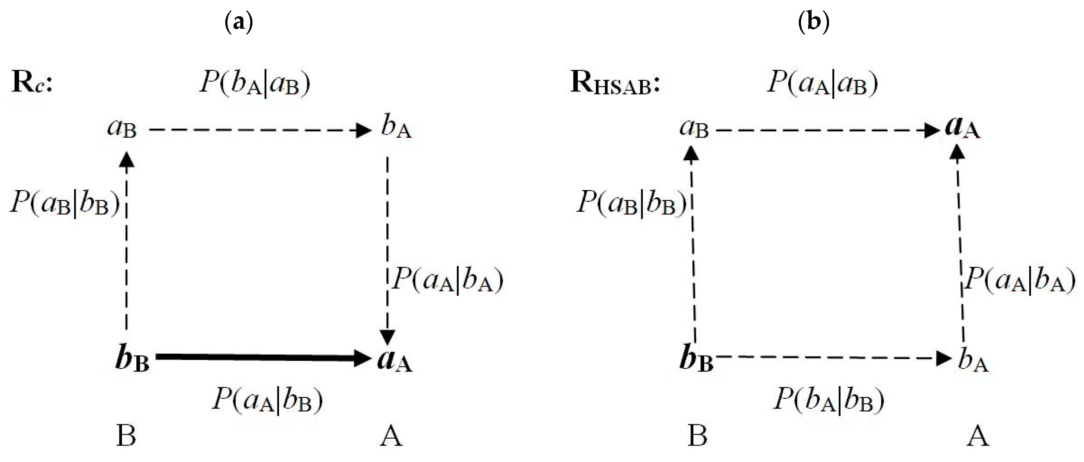
The key CT sites in both reactants determine the overall chemical character of these subsystems in reactive complexes: the acceptor (acidic) site in A, aA, and the donor (basic) site in B, bB. These crucial fragments are accentuated by the bold symbols in Figure 3, where the dominating communications between the nearest neighbors in both coordinations are shown. The Rc diagram in the Figure 3a shows that only the complementary arrangement exhibits the direct communication bB→aA, reflected by a high conditional probability Pc(bB→aA), besides the double-cascade propagation bB→[aB→bA]→aA of a relatively low probability,
The RHSAB coordination Figure 3b generates two indirect (single-cascade) scatterings between the crucial sites aA and bB:
Pc(bB→[aB→bA]→aA) = Pc(bB→aB) Pc(aB→bA) Pc(bA→aA) << Pc(bB→aA).
PHSAB(bB→aB→aA) = PHSAB(bB→aB) PHSAB(aB→aA) and
PHSAB(bB→bA→aA) = PHSAB(bB→bA) PHSAB(bA→aA).
PHSAB(bB→bA→aA) = PHSAB(bB→bA) PHSAB(bA→aA).
As indicated above, in communication theory the indirect scatterings involve products of the relevant direct propagations. Therefore, the conditional probability of the direct step bB→aA in Rc must dominate over all indirect communications between these sites. This provides additional rationale for the observed complementary preference in the acid-base coordination.
Moreover, the soft (basic) fragment is predicted to overlap with the neighboring sites more strongly compared to the hard (acidic) fragment, thus giving rise to stronger electron communications:
The strongest communications are thus expected for most covalently-bonded neighboring fragments bA and bB in the HSAB complex, while the weakest propagations are predicted between its two hard (acidic) sites aA and aB, which bind more ionically:
In RHSAB, this qualitative analysis thus suggests a covalent character of the chemical bond between the basic sites of both reactants, and the ionic bond between their acidic groups. In Rc, one similarly predicts a strong coordination bond between aA and bB, and a predominantly covalent bond between aB and bA.
Pα(bX→λ) > Pα(aX→λ) and Pα(λ→bX) > Pα(λ→aX).
P(bB→bA) >> P(aB→aA).
The current density j(r) [see Equation (37)] reflects the flow of electronic probability density p(r) with an effective velocity measuring the current-per-particle: V(r) = j(r)/p(r). It implies the associated flux of the system resultant gradient-information, JI(r) = I(r)V(r). Here, I(r) = Ip(r) + Iϕ(r) denotes the density-per-electron of the overall information combining the classical contribution Ip(r) = [∇lnp(r)]2 and its nonclassical supplement Iϕ(r) = [2∇ϕ(r)]2 due to the state phase component [see Equation (43)]. The information continuity equation then predicts the vanishing classical contribution to the resultant information source and a finite production of its nonclassical part [62,63,64,67,73].
The shifts in electron populations on active sites of donor–acceptor systems [Equation (48)] also imply the associated redistributions of the system resultant gradient-information. The concerted flows in Rc redistribute the information density more evenly, compared to a more localized redistribution in RHSAB, where electronic flows net transport the information between the key sites of both reactants: from bB to aA. The complementary coordination thus corresponds to a lower level of the overall determinicity-information [see Equation (53)] compared to that in HSAB-type coordination. Therefore, the former reactive system represents more information uncertainty in comparison to the latter complex, thus exhibiting a higher resultant gradient-entropy (indeterminicity-information).
9. Conclusions
To paraphrase Progogine [96], the classical, modulus component of molecular wavefunction determines the electronic probability distribution—the state structure of “being”—while the gradient of the nonclassical phase variable generates the current density—the system structure of “becoming”. In this work, we have explored in some detail the mutual relation between the phase component of electronic wavefunction and its current descriptor, expressing the former as an indefinite integral over the probability velocity field. The probability and current descriptors of electronic states are both related by the quantum continuity relations implied by SE of molecular QM, which have also been summarized. The optimum distribution of the state electronic density is determined by density variational principle for the system electronic energy, while the equilibrium current density results from the subsidiary extremum rule for the nonclassical entropy or information measure, which determines the state optimum phase for the given electron density. The elementary chemical processes have also been monitored using the classical entropy/information descriptors [97,98,99,100].
In phenomenological approaches to chemical reactivity, it is customary to distinguish the mutually bonded (open, entangled) and nonbonded (closed, disentangled) status of the of electronic distributions in subsystems. The former reflects the quantum state of the whole reactive system, while the latter refers to states of the mutually closed reactants. The bonded or nonbonded/frozen character of molecular fragments at such hypothetical reaction stages also delineates the allowed types of electronic communications between substrates, which are responsible for the interreactant chemical bond: the promolecular reference state R0 = (A0 | B0), describing the “frozen” (molecularly placed) electron distributions in the ground-states of separate reactants {X0}, does not allow for any communications between the system constituent AIM or their basis functions; the polarized reactive system R+ = (A+ | B+) opens internal communications within each reactant, while the final equilibrium, fully “relaxed” molecular system R* = (A* ¦ B*) already accounts for all intra- and inter-substrate propagations.
We have also demonstrated that the global equilibrium in R* establishes a common phase component of the fragment states (see Appendix C). In other words, the bonded status of molecular fragments implies the phase equalization of the effective subsystem states, at the equilibrium phase related to the “molecular” electron distribution, in the interacting system as a whole. Therefore, the bonding (entangling) of molecular fragments represents the phase-phenomenon reflecting their common (molecular) electronic state, past or present (see Appendix D). This phase equalization is independent of the actual distance between subsystems, thus representing a long-range correlation effect.
The coherence of electronic currents has also been shown to play a crucial role in establishing the energetic preference of the least-activated complementary reactive complex combining the donor and acceptor substrates. Alternative coordinations of such reactants in Rc and RHSAB complexes, respectively, imply different patterns of the dominating electronic currents and communications. The specific redistributions of the system electronic and information densities, via P and/or CT, channels, have been qualitatively discussed and the resultant pattern of the site currents have been established. We have also examined energetic implications of the overall and partial P/CT electron flows in A---B complexes using the chemical potential (electronegativity) and hardness/softness descriptors of reactants and their active sites, defined in the DFT based reactivity theory.
The phase equalization in the mutually open subsystems provides a consistent theoretical framework for distinguishing the mutually bonded and nonbonded states of their electron distributions. This IT phase criterion of electronic equilibria in molecular systems complements the familiar energetic principle of the chemical-potential (electronegativity) equalization. The complete set of requirements for the quantum equilibrium in the bonded reactive system thus calls for equalizations of both the modulus (probability) and phase (current) related (local) intensities, the chemical potentials and phases of molecular substrates, at the corresponding global descriptors characterizing the reactive system as a whole.
Thus, for the given probability distributions of subsystems, it is the equalized, “molecular” phase of the whole reactive system which marks the bonded (equilibrium) state in the reaction substrates. The phase component of molecular electronic states thus emerges as an important “association” fabric in chemical systems, which “glues” reactants in their “bonded” (entangled) condition. It keeps the “memory” of the present or past interactions between subsystems, and it shapes the probability fluxes between the substrate active sites, which effect the information flows in the reactive system.
Funding
This research received no external funding.
Conflicts of Interest
The author declares no conflict of interest.
Appendix A. Continuity Relations Revisited
The dynamics of electronic states is determined by SE, which also implies specific rates of time evolutions of both components of complex wavefunctions, and of their physical descriptors: the state probability and current distributions. The time derivatives of the modulus and phase parts of electronic states reflect the relevant continuity equations in molecular QM. For simplicity, let us consider a single electron in state |Ψ(t)〉 at time t, or the associated (complex) wavefunction in position representation:
Its modulus (R) and phase (ϕ) components determine the state physical attributes of the electron probability and current densities:
The effective velocity V(r, t) of the probability “fluid” measures the current-per-particle and reflects the state phase-gradient:
ψ(r, t) = 〈r|Ψ(t)〉 = R(r, t) exp[iϕ(r, t)], ϕ(r, t) ≥ 0.
p(r, t) = ψ(r, t)*ψ(r, t) = R(r, t)2,
j(r, t) = [ħ/(2mi)] [ψ(r, t)* ∇ψ(r, t) − ψ(r, t)∇ψ(r, t)*]
= (ħ/m) p(r, t) ∇ϕ(r, t)
≡ p(r, t) V(r, t).
= (ħ/m) p(r, t) ∇ϕ(r, t)
≡ p(r, t) V(r, t).
V(r, t) = j(r, t)/p(r, t) = (ħ/m) ∇ϕ(r, t).
Equation (A1) also identifies the two (additive) components of the wavefunction logarithm:
which determine resultant measures of the global and gradient content of the state entropy or information. For example, the complex entropy descriptor [59,62],
combines as its real part the Shannon entropy S[p] in probability distribution p, and the nonclassical phase supplement S[ϕ], which determines its imaginary component.
lnψ (r, t) = lnR(r, t) + iϕ(r, t),
S[ψ] = −2〈ψ|lnψ|ψ〉 = − 2∫p [lnR + i ϕ] dr
≡ S[p] + i S[ϕ],
≡ S[p] + i S[ϕ],
The corresponding Fisher-type measure of the state resultant gradient information I[ψ] or entropy M[ψ] are defined by expectation values of the associated (Hermitian) operators [53,54,55,56,57,58,59,60,61,62]
The former is thus related to the state average kinetic energy of electrons, T[ψ] = 〈ψ|T|ψ〉, determined by the quantum operator T = −ħ2/(2m) Δ = [ħ2/(8m)] I:
I = −4Δ = 4[(∇lnR)2 − (i∇ϕ)2] = 4[(∇lnR)2 + (∇ϕ)2] = 4|∇lnψ| and
M = 4[(∇lnR)2 + (i∇ϕ)2],
M = 4[(∇lnR)2 + (i∇ϕ)2],
I[ψ] = 〈ψ|I|ψ〉 = 4∫R2[(∇lnR)2 + (∇ϕ)2] dr = 4∫[(∇R)2 + (R ∇ϕ)2] dr ≡ I[R] + I[ϕ]
= ∫p[(∇lnp)2 + 4(∇ϕ)2] dr = ∫p−1(∇p)2 dr + 4∫p (∇ϕ)2 dr ≡ I[p] + I[ϕ],
= ∫p[(∇lnp)2 + 4(∇ϕ)2] dr = ∫p−1(∇p)2 dr + 4∫p (∇ϕ)2 dr ≡ I[p] + I[ϕ],
M[ψ] = 〈ψ|M|ψ〉 = 4{〈ψ|(∇lnR)2|ψ〉 + 〈ψ|(i∇ϕ)2|ψ〉} = I[p] − I[ϕ]
= 4∫[(∇R)2 − (∇ϕ)2] dr ≡ M[R] + M[ϕ]
= ∫p[(∇lnp)2 − 4(∇ϕ)2] dr = M[p] + M[ϕ].
= 4∫[(∇R)2 − (∇ϕ)2] dr ≡ M[R] + M[ϕ]
= ∫p[(∇lnp)2 − 4(∇ϕ)2] dr = M[p] + M[ϕ].
I[ψ] = (8m/ħ2) T[ψ] ≡ σT[ψ].
This proportionality allows one to use the molecular virial theorem [66] in general considerations on the information redistribution in the bond-formation process and during chemical reactions [67,68,69,70]. It follows from Equations (A6)–(A9) that the independent additive components of Equation (A5) indeed determine the average values of the resultant entropy/information descriptors of molecular electronic states, with the local IT densities being weighted by the state electron probability distribution.
In the molecular scenario, the electron is moving in the external potential v(r) due to the “frozen” nuclear frame of the familiar Born–Oppenheimer approximation. The electronic Hamiltonian
determines the quantum dynamics of electronic states expressed by SE,
which can be also formulated in terms of the (unitary) evolution operator
This equation and its complex conjugate then imply the associated temporal evolutions of the wavefunction components R and ϕ (see also Appendix B):
H(r) = − [ħ2/(2m)] Δ + v(r) ≡ T(r) + v(r),
iħ (∂ψ/∂t) = Hψ,
U(t − t0) ≡ U(τ) = exp(−iħ−1τ H),
ψ(t) = U(τ) ψ(t0).
∂R/∂t = −∇R·V,
∂ϕ/∂t = [ħ/(2m)] [R−1ΔR − (∇ϕ)2] − v/ħ.
These dynamical equations can be ultimately recast as the corresponding continuity relations. Consider first the continuity of probability distribution:
The divergence of probability flux of Equation (A3)
further implies the vanishing divergence of the velocity field V related to ∇2ϕ = Δϕ:
∂p/∂t = 2R (∂R/∂t) = − (2R ∇R)·V = − ∇p·V = − ∇·j or
σp ≡ dp/dt = ∂p/∂t + ∇· j = ∂p/∂t + ∇p · V = 0.
σp ≡ dp/dt = ∂p/∂t + ∇· j = ∂p/∂t + ∇p · V = 0.
∇· j = ∇p · V + p ∇·V = ∇p ·V,
∇·V = (ħ/m) Δϕ = 0 or Δϕ = 0.
The total time-derivative dp(r)/dt determines the vanishing local probability “source”: σp(r) = 0. It measures the time rate of change in an infinitesimal volume element of probability fluid moving with velocity V = dr/dt, while the partial derivative ∂p[r(t), t]/∂t refers to volume element around the fixed point in space. Indeed, separating the explicit time dependence of p(r, t) from its implicit dependence through the particle position r(t), p(r, t) = p[r(t), t], gives:
σp(r, t) = ∂p[r(t), t]/∂t + (dr/dt) · ∂p(r, t)/∂r
= ∂p(r, t)/∂t + V(r, t) ·∇p(r, t) = ∂p(r, t)/∂t + ∇· j(r, t) = 0.
= ∂p(r, t)/∂t + V(r, t) ·∇p(r, t) = ∂p(r, t)/∂t + ∇· j(r, t) = 0.
Turning now to the phase dynamics of Equation (A16), one first realizes that the effective velocity V of the probability-current j = pV also determines the phase-flux and its divergence:
This complementary flow descriptor ultimately generates a finite phase-source:
Using Equation (A16) eventually gives:
J = ϕ V and ∇· J = ∇ϕ ·V = (ħ/m) (∇ϕ)2.
σϕ ≡ dϕ/dt = ∂ϕ/∂t + ∇· J = ∂ϕ/∂t + V · ∇ϕ ≠ 0.
σϕ = [ħ/(2m)][R−1ΔR + (∇ϕ)2] − v/ħ.
To summarize, the effective velocity of probability-current also determines the phase-flux in molecules. The source (net production) of the classical probability-variable of electronic states identically vanishes, while that of their nonclassical, phase-part, determined by state components (p,ϕ) and the system external potential v, remains finite.
The local production of electronic current j = p Vis also of interest,
where we have recognized Equation (A17). A reference to Equations (A3) and (A17) then gives:
Hence, using Equation (A23) finally gives:
σj ≡ dj/dt = σp V + p (dV/dt) = p (dV/dt),
σj = (ħ/m) p d/dt(∇ϕ) = (ħ/m) p ∇(dϕ/dt) = (ħ/m) p ∇σϕ.
σj = [ħ2/(2m2)] [R ∇3R − (ΔR) ∇R] − (p/m) ∇v.
Appendix B. Schrödinger Equation and Wavefunction Components
Let us now examine the implications of the (complex) SE [Equation (A12)] when expressed in terms of the modulus and phase components of wavefunction [see Equation (A1)]:
where we use Equation (A19). Multiplying both sides of this equation by exp(−iϕ) and dividing by ħR finally gives:
iħ (∂ψ/∂t) = iħ [(∂R/∂t) + iR(∂ϕ/∂t)] exp(iψ)
= Hψ = {−[ħ2/(2m)] [ΔR + 2i∇R·∇ϕ − R(∇ϕ)2] + vR} exp(iϕ),
= Hψ = {−[ħ2/(2m)] [ΔR + 2i∇R·∇ϕ − R(∇ϕ)2] + vR} exp(iϕ),
i (∂lnR/∂t) − (∂ϕ/∂t) = −[ħ/(2m)] [R−1ΔR + 2i(∇lnR)·∇ϕ − (∇ϕ)2] + v/ħ.
Comparing the imaginary parts of the preceding equation generates the dynamic equation for the time evolution of the modulus part of electronic state,
which can be directly transformed into the probability continuity equation (A17):
∂lnR/∂t = − [(ħ/m) ∇ϕ] ·∇lnR = − V·∇lnR,
∂p/∂t = −∇· j or σp = dp/dt = 0.
Equating the real parts of Equation (A27) similarly determines the phase-dynamics of Equation (A16):
The latter equation also determines the phase-production σϕ = dϕ/dt [Equation (A23)] for its flux definition of Equation (A21), in the phase continuity relation:
∂ϕ/∂t = [ħ/(2m)] [R−1ΔR − (∇ϕ)2] − v/ħ.
∂ϕ/∂t = −∇· J+ σϕ.
The average electronic energy in state (A1) thus combines the following component contributions:
where we use the relevant integration by parts and 〈Vne〉ψ denotes the state average electron-nuclei attraction energy. The phase-dependent part of the average kinetic energy 〈T〉ψ identically vanishes in the stationary electronic state
for the sharply specified electronic energy
when ϕs(t) = − (Es/ħ) t ≡ − ωst and hence ∇ϕs(t) = 0.
〈E〉ψ = 〈ψ|H|ψ〉 = −[ħ2/(2m)] ∫[RΔR − R2(∇ϕ)2] dr + ∫R2 v dr
= [ħ2/(2m)] ∫[(∇R)2 + R2(∇ϕ)2]dr + ∫R2 v dr ≡ 〈T〉ψ + 〈Vne〉ψ,
= [ħ2/(2m)] ∫[(∇R)2 + R2(∇ϕ)2]dr + ∫R2 v dr ≡ 〈T〉ψ + 〈Vne〉ψ,
ψs(r, t) = Rs(r) exp[iϕs(t)],
Es = Rs(r)−1 H(r) Rs(r) = − [ħ2/(2m)] Rs(r)−1ΔRs(r) + v(r) = const.,
The open systems and their fragments are described by grand ensembles and exhibit continuously varying, fractional average numbers of electrons; the closed molecules and their parts similarly exhibit integer numbers of electrons. The pure state ΨR*(N,t0) of the whole externally-closed but internally-open reactive complex R* = (A* ¦ B*) at time t0 ≡ 0, defined by its overall external potential v = vA + vB and number of electrons N = NA + NB (integer), can be expanded
in terms of the complete set of the system stationary states, the eigensolutions
of N-electron molecular Hamiltonian:
Here, Rs(N) denotes the time-independent amplitude (modulus) function of N electrons, while T(N), Vne(N) and Uee(N) stand for the quantum operators of electronic kinetic, attraction and repulsion energies, respectively. Given the state Ψ(N, t0) at the initial time t0 = 0, its form at time τ [see Equations (A13) and (A14)] is determined by the interval evolution operator
where Ψs(N, τ) = Rs(N) exp[iϕs(τ)] is the full stationary state of N-electrons corresponding to energy Es.
ΨR*(N, t0) = Σs Cs(t0) Rs(N), Cs(t0) = 〈Rs(N)|ΨR*(N, t0)〉,
H(N) Rs(N) = Es Rs(N)
H(N) = T(N) + Vne(N) + Uee(N),
T(N) = Σk T(k), Vne(N) = Σk v(k), Uee(N) = Σk<l g(k, l).
T(N) = Σk T(k), Vne(N) = Σk v(k), Uee(N) = Σk<l g(k, l).
U(τ, N) = exp[−iħ−1τ H(N)],
Ψ(N, τ) = U(τ) Ψ(N, t0) = Σs Cs(t0) {exp[iϕs(τ)] Rs(N)}
≡ Σs Cs(t0) Ψs(N, τ),
≡ Σs Cs(t0) Ψs(N, τ),
Such pure-state expansion is not available for the open systems in their final (mixed) equilibrium states, described by the fragment density operators defining the associated ensembles of Hamiltonians for different numbers of electrons. At the polarization stage R+ = (A+ | B+), however, involving the mutually- and externally-closed substrates, each subsystem X+ conserves the initial (integer) number of electrons NX0 so that the interacting-fragment Hamiltonians {HX(NX0)} for the overall external potential v of the whole system are well defined, e.g.,
They determine the stationary eigenproblems for subsystems containing the initial, integer numbers of electrons in separate reactants,
and associated expansions at time t0 of general states in the polarized subsystems:
Their evolution in time interval τ is determined by the reactant operators
where
denotes the stationary phase of subsystem X+, while
stands for the full stationary state of reactant X in presence of the other substrate, corresponding to the fragment energy Eu(X+).
HA(NA0) = T(NA0) + Vne(NA0) + UA(NA0) + UAB(NA0, NB0),
UA(NA0) = Σ(k<l)∈ A g(k, l), UAB(NA0, NB0) = Σk∈ AΣl∈ B g(k, l), etc.
UA(NA0) = Σ(k<l)∈ A g(k, l), UAB(NA0, NB0) = Σk∈ AΣl∈ B g(k, l), etc.
HX(NX0) φu(NX0) = Eu(X+) φu(NX0), X = A, B,
ΨX+(NX0, t0) = Σu Cu(X+, t0) φu(NX0), Cu(X+, t0) = 〈φu(NX0)|ΨX+(NX0, t0)〉.
UX(τ, NX0) = exp[−iħ−1τ HX(NX0)], X = A, B,
ΨX+(NX0, τ) = UX(τ, NX0) ΨX+(NX0, t0)
= Σu Cu(X+, t0) {exp[iϕu(X+, τ)] φu(NX0)}
≡ Σu Cu(X+, t0) Φu(NX0, τ),
= Σu Cu(X+, t0) {exp[iϕu(X+, τ)] φu(NX0)}
≡ Σu Cu(X+, t0) Φu(NX0, τ),
ϕu(X+,τ) = − [Eu(X+)/ħ] τ ≡ − ωu(X+)τ
Φu(NX0, τ) = φu(NX0) exp[iϕu(X+, τ)]
Products of such stationary wavefunctions of both fragments, describing their distinguishable groups of electrons,
thus constitute the complete basis for expanding general electronic states of the polarized reactive system R+ [compare Equation (A39)]:
{Θu,w(A+, B+; τ) = Φu(NA0, τ) Φw(NB0, τ)
= φu(NA0) φw(NB0) exp{i[ϕu(A+,τ) + ϕw(B+,τ)]}
≡ ϑu,w(NA0, NB0) exp[iθu,w(τ)]},
= φu(NA0) φw(NB0) exp{i[ϕu(A+,τ) + ϕw(B+,τ)]}
≡ ϑu,w(NA0, NB0) exp[iθu,w(τ)]},
θu,w(τ) = −ħ−1[Eu(A+) + Ew(B+)]τ = −[ωu(A+) + ωw(B+)] τ = −ωu,w τ,
ΨR+(N, τ) = Σu,w Du,v(t0) {exp[iθu,w(τ)]ϑu,w(NA0, NB0)}
= Σu,w Du,v(t0) Φu(NA0, τ) Φw(NB0, τ)
= Σu,w Du,v(t0) Θu,w(A+, B+; τ),
Du,v(t0) = 〈ϑu,w(NA0, NB0)|ΨR+(N, t0)〉.
= Σu,w Du,v(t0) Φu(NA0, τ) Φw(NB0, τ)
= Σu,w Du,v(t0) Θu,w(A+, B+; τ),
Du,v(t0) = 〈ϑu,w(NA0, NB0)|ΨR+(N, t0)〉.
While stationary states of the whole reactive system imply the purely time-dependent phase, the effective (mixed) states of reactants X* in R* = (A*¦B*), identified by their partial densities {ρX* = NX*pX*, NX* = ∫ρX*dr (fractional)}, pieces of molecular electron density
exhibit the local phases generating nonvanishing phase gradients. Indeed, the HZM construction [73,74,75,76] of wavefunctions yielding the prescribed probability distributions {pX*} on subsystems gives rise to finite electronic currents on reactants. This current pattern in both substrates or on their acidic and basic sites manifests the valence-state activation of such open fragments, which generates nonvanishing contributions to the associated (nonclassical) entropy/information descriptors.
ρR* = ρA* + ρB*,
Appendix C. Information Principle
The partial currents {jα(r, λ)} and probability distributions {pα(r, λ)} in active fragments
of the reactive system Rα, α = (c, HSAB), determine the additive site contributions to the resultant (nonclassical) gradient-information [see Equations (43) and (A8)] in Rα:
λ ∈ (aA =1, bA = 2, aB = 3, bB = 4)
Iα[{jα(λ)}] = Σλ Iαλ[jα(λ)], Iαλ[jα(λ)] = (2m/ħ)2 ∫pα(r, λ)−1 jα(r, λ)2 dr.
The minimum of this current-determinicity measure Iα[{jα(λ)}] implies the maximum of the complementary nonclassical current-indeterminicity descriptor, of the site gradient “entropy” [Equation (A9)] containing negative nonclassical contribution [62,63]. Consider such a nonclassical information principle subject to the local constraint of preserving the resultant local current in Rα,
where the vector Lagrange multiplier ξα(r) enforces the local constraint of Equation (A53). The Euler equations determining the optimum site-currents then read:
jα(r) = Σλjα(r, λ),
δ{Iα[{jα(λ)}] − ∫ξα(r)·jα(r) dr} = 0,
δIα[{jα(λ)}]/δjα(r, λ) = (8m2/ħ2) [jα(r, λ)/pα(r, λ)] ≡ (8m2/ħ2) Vα(r, λ) = ξα(r).
Therefore, at the minimum of the current-information the fragment equilibrium (eq.) probability-velocity is λ-independent,
Moreover, since this effective velocity descriptor is determined by the phase gradients of Equations (37) and (44), one concludes from the preceding equation that the equilibrium phases {ϕα(r, λ)} of the site “states” can differ only by a constant, irrelevant in QM, thus containing the same (site “equalized”) local contribution. The minimization of the nonclassical gradient information thus gives rise to the site phase-equalization in the information-equilibrium state of the reactive system as a whole [63].
Vα(r, λ) = [ħ2/(8m2)] ξα(r) ≡ Vαeq.(r).
Appendix D. Reactant Entanglement
The A and B subsystems of the reactive system R = A—B ultimately represent the bonded (entangled) subsystems in the equilibrium complex R* = (A* ¦ B*) containing the mutually- and internally-open substrates {X*}. Therefore, when brought into temporary interaction and then infinitely separated in R*(∞) = A* + B*, such dissociated fragments can no longer be described by the individual wavefunctions for each reactant, even after the interaction has utterly ceased and the “molecular” Hamiltonian is given by the sum of subsystem Hamiltonians:
Indeed, QM deals with a tensor product of subsystem spaces, not with their sum [101]. However, for additive parts of the Hamiltonian, the “separation theorem” of QM predicts
so that the following natural question arises: What is the molecular trace (“memory”) of the past interaction left in the entangled separated fragments? As we have already argued elsewhere, it is the phase part of the system wavefunction which preserves a memory of the temporary interaction between subsystems (see also Appendix C).
H[R(∞)] = H(A) + H(B).
Ψ[R(∞)] = Ψ(A) Ψ(B),
The IT equilibrium phase of the given quantum system as a whole has been previously linked to its probability distribution p(r) [62,63], ϕeq.(r) = − (½) lnp(r), thus predicting the equilibrium current proportional to the negative gradient of probability density [see Equation (37)]:
Therefore, the product function in Equation (A57) of the separated “dissociated” subsystems still preserves the memory of the probability distribution p(r) of the past (interacting) subsystems at a finite separation between reactants, contained in the equilibrium phase for this “molecular” separated reactive system.
jeq.(r) = (ħ/m) p(r) ∇ϕeq.(r) ≡ p(r) Veq.(r) = − [ħ/(2m)] ∇p(r).
The same phase criterion applies to diagnosing the entanglement distinction between the bonded and nonbonded status of reactants in the equilibrium, R* = (A* ¦ B*), and polarized, R+ = (A | B), complexes, respectively. For the same probability distribution pR(r) in both these hypothetical states, the two subsystems are free to exchange electrons in the former, while in the latter this flow of electrons is forbidden. The equilibrium phase of Ψ(R*) then reflects the negative of lnpR, ϕeq.(R*) = ϕeq.[pR], while at a finite separation RAB between reactants ϕeq.(R+) is proportional to the negative of ln[(pApB)1/2]. Therefore, it is also the phase component which distinguishes the bonded (entangled) state of reactants in R* from their nonbonded (disentangled) status in R+, also at finite separations between the two reactants.
The mutual opening of the interacting reactants at their finite separation establishes the state global phase ϕeq.[R*(xAB)], where xAB denotes the separation coordinate, which is naturally transformed in the dissociation limit RAB→∞ into the equilibrium phases of reactants,
upon the infinite separation of the mutually open subsystems, when
ϕeq.[R*(RAB→∞)]→{ϕeq.[A*(xAB → −∞)] or ϕeq.[B*(xAB → +∞)]},
ρR[R*(RAB→∞)] → {ρA*(xAB → −∞) or ρB*(xAB → +∞)}.
Appendix E. Density Matrices for Interacting Subsystems
In describing the mixed states of interacting subsystems, it is useful to apply the density matrix formalism of QM [102,103]. Consider again the acid and base reactants in the polarized (interacting) system R+ = [A+(x)|B+(ξ)], where x and ξ denote their internal coordinates, respectively. For example, in the topological, physical-space partitioning [104] of the molecular electron density, into pieces belonging to separate basins of the physical space, these coordinates describe the disjoint sets of the position variables in these regions of space, while in the functional-space division schemes, e.g., the stockholder partition [21], each of these coordinates explores the whole physical space of the allowed positions of the separate groups of electrons.
The physical properties of subsystems are represented by quantum operators acting on the internal degrees-of-freedom of the fragment in question. Since R+ as a whole is assumed to represent an isolated system, it is described by the specific wavefunction Ψ(x, ξ), the pure quantum state of the reactive system. For example, the interacting-fragment Hamiltonians in R+, {HX(NX0)} act on the position variables of NX0 electrons belonging to X+. The stationary states of HA(NA0) ≡ HA(x),
form the complete set capable of expanding the state of the whole system:
Notice, however, that the simple product representation of Ψ(x, ξ) is not available at finite separations, between interacting subsystems, so that the state of each reactant cannot be described by the substrate wavefunction dependent on its own internal coordinates.
HA(x) φs(x) = Es(A+) φs(x),
Ψ(x, ξ) = Σs Φs(ξ) φs(x), Φs(ξ) = ∫φs*(x) Ψ(x, ξ) dx.
The quantum operator of the physical property L(A) of subsystem A+ will act only on variables x: L(A) = Lx. Its average value in the general state of Equation (A62), of the reactive system as a whole, then reads:
Here, ρ(A) = {ρs’,s} stands for the effective density matrix of subsystem A+(x), already integrated over coordinates of electrons in the complementary subsystem B+(ξ). The partial trace of the preceding equation thus enables one to calculate the ensemble average of the subsystem quantity L(A) as if this part of R+ were isolated, being in the effective mixed state defined by subsystem density matrix ρ(A) in representation {φs(x)}.
〈L〉Ψ = ∫∫Ψ*(x, ξ) Lx Ψ(x, ξ) dx dξ
= ΣsΣs’ [∫Φs’*(ξ) Φs(ξ) dξ] [∫φs’*(x) Lx φs(x) dx]
≡ Σs Σs’ ρs,s’(A) Ls’,s(A) = trA[ρ(A) L(A)].
= ΣsΣs’ [∫Φs’*(ξ) Φs(ξ) dξ] [∫φs’*(x) Lx φs(x) dx]
≡ Σs Σs’ ρs,s’(A) Ls’,s(A) = trA[ρ(A) L(A)].
Writing the preceding equation in the subsystem position representation,
where 〈x’|Lx|x〉 = Lxδ(x’ − x), one obtains the following expression for the subsystem density matrix:
These expressions for the expectation values of subsystem operators in the mixed quantum states are independent of the applied representation. The corresponding dynamics of the reactant density matrices involved are also uniquely determined by molecular SE.
〈L〉Ψ = ∫∫ρA(x, x’) 〈x’|Lx|x〉 dx dx’,
ρA(x, x’) = ∫Ψ*(x’, ξ) Ψ(x, ξ) dξ = ΣsΣs’ ρs,s’(A) φs’*(x’) φs(x)
≡ ΣsΣs’ ρs,s’(A) Ωs’,s(x, x’) = trA[ρ(A) ΩA(x, x’)].
≡ ΣsΣs’ ρs,s’(A) Ωs’,s(x, x’) = trA[ρ(A) ΩA(x, x’)].
To summarize, also the polarized (interacting) reactants {X+} in R+ cannot be described by a single wavefunction of the pure quantum state. They have to instead be characterized by the density matrix reflecting an incoherent mixture of subsystem states, weighted by the ensemble probability factors and corresponding to the substrate mixed quantum state.
References
- Fisher, R.A. Theory of statistical estimation. Proc. Camb. Phil. Soc. 1925, 22, 700–725. [Google Scholar] [CrossRef] [Green Version]
- Frieden, B.R. Physics from the Fisher Information—A Unification; Cambridge University Press: Cambridge, UK, 2004. [Google Scholar]
- Shannon, C.E. The mathematical theory of communication. Bell Syst. Tech. J. 1948, 27, 379–493, 623–656. [Google Scholar] [CrossRef] [Green Version]
- Shannon, C.E.; Weaver, W. The Mathematical Theory of Communication; University of Illinois: Urbana, IL, USA, 1949. [Google Scholar]
- Kullback, S.; Leibler, R.A. On information and sufficiency. Ann. Math. Stat. 1951, 22, 79–86. [Google Scholar] [CrossRef]
- Kullback, S. Information Theory and Statistics; Wiley: New York, NY, USA, 1959. [Google Scholar]
- Abramson, N. Information Theory and Coding; McGraw-Hill: New York, NY, USA, 1963. [Google Scholar]
- Pfeifer, P.E. Concepts of Probability Theory; Dover: New York, NY, USA, 1978. [Google Scholar]
- Nalewajski, R.F. Information Theory of Molecular Systems; Elsevier: Amsterdam, The Netherlands, 2006. [Google Scholar]
- Nalewajski, R.F. Information Origins of the Chemical Bond; Nova Science Publishers: New York, NY, USA, 2010. [Google Scholar]
- Nalewajski, R.F. Perspectives in Electronic Structure Theory; Springer: Heidelberg, Germany, 2012. [Google Scholar]
- Nalewajski, R.F.; Parr, R.G. Information theory, atoms-in-molecules and molecular similarity. Proc. Natl. Acad. Sci. USA 2000, 97, 8879–8882. [Google Scholar] [CrossRef] [PubMed] [Green Version]
- Nalewajski, R.F. Information principles in the theory of electronic structure. Chem. Phys. Lett. 2003, 272, 28–34. [Google Scholar] [CrossRef]
- Nalewajski, R.F. Information principles in the Loge Theory. Chem. Phys. Lett. 2003, 375, 196–203. [Google Scholar] [CrossRef]
- Nalewajski, R.F.; Broniatowska, E. Information distance approach to Hammond Postulate. Chem. Phys. Lett. 2003, 376, 33–39. [Google Scholar] [CrossRef]
- Nalewajski, R.F.; Parr, R.G. Information-theoretic thermodynamics of molecules and their Hirshfeld fragments. J. Phys. Chem. A 2001, 105, 7391–7400. [Google Scholar] [CrossRef]
- Nalewajski, R.F. Hirshfeld analysis of molecular densities: Subsystem probabilities and charge sensitivities. Phys. Chem. Chem. Phys. 2002, 4, 1710–1721. [Google Scholar] [CrossRef]
- Parr, R.G.; Ayers, P.W.; Nalewajski, R.F. What is an atom in a molecule? J. Phys. Chem. A. 2005, 109, 3957–3959. [Google Scholar] [CrossRef]
- Nalewajski, R.F.; Broniatowska, E. Atoms-in-Molecules from the stockholder partition of molecular two-electron distribution. Theoret. Chem. Acc. 2007, 117, 7–27. [Google Scholar] [CrossRef]
- Heidar-Zadeh, F.; Ayers, P.W.; Verstraelen, T.; Vinogradov, I.; Vöhringer-Martinez, E.; Bultinck, P. Information-theoretic approaches to Atoms-in-Molecules: Hirshfeld family of partitioning schemes. J. Phys. Chem. A 2018, 122, 4219–4245. [Google Scholar] [CrossRef] [PubMed] [Green Version]
- Hirshfeld, F.L. Bonded-atom fragments for describing molecular charge densities. Theoret. Chim. Acta 1977, 44, 129–138. [Google Scholar] [CrossRef]
- Nalewajski, R.F. Entropic measures of bond multiplicity from the information theory. J. Phys. Chem. A 2000, 104, 11940–11951. [Google Scholar] [CrossRef]
- Nalewajski, R.F. Entropy descriptors of the chemical bond in Information Theory: I. Basic concepts and relations. Mol Phys 102:531-546; II. Application to simple orbital models. Mol. Phys. 2004, 102, 547–566. [Google Scholar] [CrossRef]
- Nalewajski, R.F. Entropic and difference bond multiplicities from the two-electron probabilities in orbital resolution. Chem. Phys. Lett. 2004, 386, 265–271. [Google Scholar] [CrossRef]
- Nalewajski, R.F. Reduced communication channels of molecular fragments and their entropy/information bond indices. Theoret. Chem. Acc. 2005, 114, 4–18. [Google Scholar] [CrossRef]
- Nalewajski, R.F. Partial communication channels of molecular fragments and their entropy/information indices. Mol. Phys. 2005, 103, 451–470. [Google Scholar] [CrossRef]
- Nalewajski, R.F. Entropy/information descriptors of the chemical bond revisited. J. Math. Chem. 2011, 49, 2308–2329. [Google Scholar] [CrossRef] [Green Version]
- Nalewajski, R.F. Quantum information descriptors and communications in molecules. J. Math. Chem. 2014, 52, 1292–1323. [Google Scholar] [CrossRef] [Green Version]
- Nalewajski, R.F. Multiple, localized and delocalized/conjugated bonds in the orbital-communication theory of molecular systems. Adv. Quantum Chem. 2009, 56, 217–250. [Google Scholar]
- Nalewajski, R.F.; Szczepanik, D.; Mrozek, J. Bond differentiation and orbital decoupling in the orbital communication theory of the chemical bond. Adv. Quantum Chem. 2011, 61, 1–48. [Google Scholar]
- Nalewajski, R.F.; Szczepanik, D.; Mrozek, J. Basis set dependence of molecular information channels and their entropic bond descriptors. J. Math. Chem. 2012, 50, 1437–1457. [Google Scholar] [CrossRef] [Green Version]
- Nalewajski, R.F. Electron communications and chemical bonds. In Frontiers of Quantum Chemistry; Wójcik, M., Nakatsuji, H., Kirtman, B., Ozaki, Y., Eds.; Springer: Singapore, 2017; pp. 315–351. [Google Scholar]
- Nalewajski, R.F.; Świtka, E.; Michalak, A. Information distance analysis of molecular electron densities. Int. J. Quantum Chem. 2002, 87, 198–213. [Google Scholar] [CrossRef]
- Nalewajski, R.F.; Broniatowska, E. Entropy displacement analysis of electron distributions in molecules and their Hirshfeld atoms. J. Phys. Chem. A 2003, 107, 6270–6280. [Google Scholar] [CrossRef]
- Nalewajski, R.F. Use of Fisher information in quantum chemistry. Int. J. Quantum Chem. 2008, 108, 2230–2252. [Google Scholar] [CrossRef]
- Nalewajski, R.F.; Köster, A.M.; Escalante, S. Electron localization function as information measure. J. Phys. Chem. A 2005, 109, 10038–10043. [Google Scholar] [CrossRef]
- Becke, A.D.; Edgecombe, K.E. A simple measure of electron localization in atomic and molecular systems. J. Chem. Phys. 1990, 92, 5397–5403. [Google Scholar] [CrossRef]
- Silvi, B.; Savin, A. Classification of chemical bonds based on topological analysis of electron localization functions. Nature 1994, 371, 683–686. [Google Scholar] [CrossRef]
- Savin, A.; Nesper, R.; Wengert, S.; Fässler, T.F. ELF: The electron localization function. Angew. Chem. Int. Ed. Engl. 1997, 36, 1808–1832. [Google Scholar] [CrossRef]
- Hohenberg, P.; Kohn, W. Inhomogeneous electron gas. Phys. Rev. 1964, 136B, 864–971. [Google Scholar] [CrossRef] [Green Version]
- Kohn, W.; Sham, L.J. Self-consistent equations including exchange and correlation effects. Phys. Rev. 1965, 140A, 133–1138. [Google Scholar] [CrossRef] [Green Version]
- Levy, M. Universal variational functionals of electron densities, first-order density matrices, and natural spin-orbitals and solution of the v-representability problem. Proc. Natl. Acad. Sci. USA 1979, 76, 6062–6065. [Google Scholar] [CrossRef] [PubMed] [Green Version]
- Parr, R.G.; Yang, W. Density-Functional Theory of Atoms and Molecules; Oxford University Press: New York, NY, USA, 1989. [Google Scholar]
- Dreizler, R.M.; Gross, E.K.U. Density Functional Theory: An Approach to the Quantum Many-Body Problem; Springer: Berlin, Germany, 1990. [Google Scholar]
- Nalewajski, R.F. (Ed.) Density Functional Theory I-IV, Topics in Current Chemistry; Springer: Berlin, Germany, 1966; Volume 180–183. [Google Scholar]
- Nalewajski, R.F.; de Silva, P.; Mrozek, J. Use of nonadditive Fisher information in probing the chemical bonds. J. Mol. Struct. 2010, 954, 57–74. [Google Scholar] [CrossRef]
- Nalewajski, R.F. Through-space and through-bridge components of chemical bonds. J. Math. Chem. 2011, 49, 371–392. [Google Scholar] [CrossRef] [Green Version]
- Nalewajski, R.F. Chemical bonds from through-bridge orbital communica-tions in prototype molecular systems. J. Math. Chem. 2011, 49, 546–561. [Google Scholar] [CrossRef] [Green Version]
- Nalewajski, R.F. On interference of orbital communications in molecular systems. J. Math. Chem. 2011, 49, 806–815. [Google Scholar] [CrossRef] [Green Version]
- Nalewajski, R.F.; Gurdek, P. On the implicit bond-dependency origins of bridge interactions. J. Math. Chem. 2011, 49, 1226–1237. [Google Scholar] [CrossRef] [Green Version]
- Nalewajski, R.F. Direct (through-space) and indirect (through-bridge) components of molecular bond multiplicities. Int. J. Quantum Chem. 2012, 112, 2355–2370. [Google Scholar] [CrossRef]
- Nalewajski, R.F.; Gurdek, P. Bond-order and entropic probes of the chemical bonds. Struct. Chem. 2012, 23, 1383–1398. [Google Scholar] [CrossRef] [Green Version]
- Nalewajski, R.F. Exploring molecular equilibria using quantum information measures. Ann. Phys. 2013, 525, 256–268. [Google Scholar] [CrossRef]
- Nalewajski, R.F. On phase equilibria in molecules. J. Math. Chem. 2014, 52, 588–612. [Google Scholar] [CrossRef] [Green Version]
- Nalewajski, R.F. Quantum information approach to electronic equilibria: Molecular fragments and elements of non-equilibrium thermodynamic description. J. Math. Chem. 2014, 52, 1921–1948. [Google Scholar] [CrossRef] [Green Version]
- Nalewajski, R.F. Phase/current information descriptors and equilibrium states in molecules. Int. J. Quantum Chem. 2015, 115, 1274–1288. [Google Scholar] [CrossRef] [Green Version]
- Nalewajski, R.F. Quantum information measures and molecular phase equilibria. In Advances in Mathematics Research; Baswell, A.R., Ed.; Nova Science Publishers: New York, NY, USA, 2015; Volume 19, pp. 53–86. [Google Scholar]
- Nalewajski, R.F. On phase/current components of entropy/information descriptors of molecular states. Mol. Phys. 2014, 112, 2587–2601. [Google Scholar] [CrossRef]
- Nalewajski, R.F. Complex entropy and resultant information measures. J. Math. Chem. 2016, 54, 1777–1782. [Google Scholar] [CrossRef] [Green Version]
- Nalewajski, R.F. Phase description of reactive systems. In Conceptual Density Functional Theory; Islam, N., Kaya, S., Eds.; Apple Academic Press: Waretown, NJ, USA, 2018; pp. 217–249. [Google Scholar]
- Nalewajski, R.F. Quantum information measures and their use in chemistry. Curr. Phys. Chem. 2017, 7, 94–117. [Google Scholar] [CrossRef]
- Nalewajski, R.F. Quantum Information Theory of Molecular States; Nova Science Publishers: New York, NY, USA, 2016. [Google Scholar]
- Nalewajski, R.F. Resultant information approach to donor-acceptor systems. In An Introduction to Electronic Structure Theory; Nova Science Publishers: New York, NY, USA, 2020; in press. [Google Scholar]
- Nalewajski, R.F. Information equilibria, subsystem entanglement and dynamics of overall entropic descriptors of molecular electronic structure. J. Mol. Model. 2018, 24, 212–227. [Google Scholar] [CrossRef] [Green Version]
- Nalewajski, R.F. On entangled states of molecular fragments. Trends Phys. Chem. 2016, 16, 71–85. [Google Scholar]
- Nalewajski, R.F. Virial theorem implications for the minimum energy reaction paths. Chem. Phys. 1980, 50, 127–136. [Google Scholar] [CrossRef]
- Nalewajski, R.F. Understanding electronic structure and chemical reactivity: Quantum-information perspective. Appl. Sci. 2019, 9, 1262–1292, In The Application of Quantum Mechanics to the Reactivity of Molecules. [Google Scholar] [CrossRef] [Green Version]
- Nalewajski, R.F. Overall Entropy/Information Descriptors of Electronic States and Chemical Reactivity; Islam, N., Bir Singh, S., Ranjan, P., Haghi, A.K., Eds.; Apple Academic Press: Waretown, NJ, USA, 2020; in press. [Google Scholar]
- Nalewajski, R.F. On entropy/information description of reactivity phenomena. In Advances in Mathematics Research; Baswell, A.R., Ed.; Nova Science Publishers: New York, NY, USA, 2019; Volume 26, pp. 97–157. [Google Scholar]
- Nalewajski, R.F. Role of electronic kinetic energy (resultant gradient information) in chemical reactivity. J. Mol. Model. 2019, 25, 259–278, Berski, S., Sokalski, W.A. (Eds.). [Google Scholar] [CrossRef] [PubMed] [Green Version]
- Nalewajski, R.F. On classical and quantum entropy/information descriptors of molecular electronic states. In Research Methodologies and Practical Applications of Chemistry; Pogliani, L., Haghi, A.K., Islam, N., Eds.; Apple Academic Press: Waretown, NJ, USA, 2019; in press. [Google Scholar]
- Callen, H.B. Thermodynamics: An Introduction to the Physical Theories of Equilibrium Thermostatics and Irreversible Thermodynamics; Wiley: New York, NY, USA, 1962. [Google Scholar]
- Nalewajski, R.F. Equidensity orbitals in resultant-information description of electronic states. Theoret. Chem. Acc. 2019, 138, 108–123, In Chemical Concepts from Theory and Computation; Liu, S. (Ed.). [Google Scholar] [CrossRef] [Green Version]
- Nalewajski, R.F. Resultant information description of electronic states and chemical processes. J. Phys. Chem. A 2019, 123, 45–60. [Google Scholar] [CrossRef] [PubMed]
- Harriman, J.E. Orthonormal orbitals for the representation of an arbitrary density. Phys. Rev. A 1980, 24, 680–682. [Google Scholar] [CrossRef]
- Zumbach, G.; Maschke, K. New approach to the calculation of density functionals. Phys. Rev. A 1983, 28, 544–554, Erratum, Phys Rev A 29, 1585–1587. [Google Scholar] [CrossRef] [Green Version]
- Macke, W. Zur wellermechanischen behandlung von vielkoeperproblemen. Ann. Phys. 1955, 17, 1–9. [Google Scholar] [CrossRef]
- Gilbert, T.L. Hohenberg-Kohn theorem for nonlocal external potentials. Phys. Rev. B 1975, 12, 2111–2120. [Google Scholar] [CrossRef]
- Nalewajski, R.F.; Korchowiec, J.; Michalak, A. Reactivity criteria in charge sensitivity analysis. Top. Curr. Chem. 1996, 183, 25–141, In Density Functional Theory IV; Nalewajski, R.F., Ed. [Google Scholar]
- Nalewajski, R.F.; Korchowiec, J. Charge Sensitivity Approach to Electronic Structure and Chemical Reactivity; World Scientific: Singapore, 1997. [Google Scholar]
- Geerlings, P.; De Proft, F.; Langenaeker, W. Conceptual density functional theory. Chem. Rev. 2003, 103, 1793–1873. [Google Scholar] [CrossRef]
- Nalewajski, R.F. Sensitivity analysis of charge transfer systems: In situ quantities, intersecting state model and its implications. Int. J. Quantum Chem. 1994, 49, 675–703. [Google Scholar] [CrossRef]
- Nalewajski, R.F. Charge sensitivity analysis as diagnostic tool for predicting trends in chemical reactivity. In Proceedings of the NATO ASI on Density Functional Theory; (Il Ciocco, 1993); Dreizler, R.M., Gross, E.K.U., Eds.; Plenum: New York, NY, USA, 1995; pp. 339–389. [Google Scholar]
- Chattaraj, P.K. (Ed.) Chemical Reactivity Theory: A Density Functional View; CRC Press: Boca Raton, FL, USA, 2009. [Google Scholar]
- Nalewajski, R.F. Chemical reactivity description in density-functional and information theories. Acta Phys. Chim. Sin. 2017, 33, 2491–2509, In Chemical Concepts from Density Functional Theory; Liu, S.(Ed.). [Google Scholar]
- Gyftopoulos, E.P.; Hatsopoulos, G.N. Quantum-thermodynamic definition of electronegativity. Proc. Natl. Acad. Sci. USA 1965, 60, 786–793. [Google Scholar] [CrossRef] [PubMed] [Green Version]
- Perdew, J.P.; Parr, R.G.; Levy, M.; Balduz, J.L. Density functional theory for fractional particle number: Derivative discontinuities of the energy. Phys. Rev. Lett. 1982, 49, 1691–1694. [Google Scholar] [CrossRef]
- Mulliken, R.S. A new electronegativity scale: Together with data on valence states and on ionization potentials and electron affinities. J. Chem. Phys. 1934, 2, 782–793. [Google Scholar] [CrossRef]
- Iczkowski, R.P.; Margrave, J.L. Electronegativity. J. Am. Chem. Soc. 1961, 83, 3547–3551. [Google Scholar] [CrossRef]
- Parr, R.G.; Donnelly, R.A.; Levy, M.; Palke, W.E. Electronegativity: The density functional viewpoint. J. Chem. Phys. 1978, 69, 4431–4439. [Google Scholar] [CrossRef]
- Parr, R.G.; Pearson, R.G. Absolute hardness: Companion parameter to absolute electronegativity. J. Am. Chem. Soc. 1983, 105, 7512–7516. [Google Scholar] [CrossRef]
- Parr, R.G.; Yang, W. Density functional approach to the frontier-electron theory of chemical reactivity. J. Am. Chem. Soc. 1984, 106, 4049–4050. [Google Scholar] [CrossRef]
- Dirac, P.A.M. The Principles of Quantum Mechanics; Oxford University Press: Oxford, UK, 1967. [Google Scholar]
- Chandra, A.K.; Michalak, A.; Nguyen, M.T.; Nalewajski, R.F. On regional matching of atomic softnesses in chemical reactions: Two-reactant charge sensitivity study. J. Phys. Chem. A 1998, 102, 10182–10188. [Google Scholar] [CrossRef]
- Nalewajski, R.F. Manifestations of the maximum complementarity principle for matching atomic softnesses in model chemisorption systems. Top. Catal. 2000, 11, 469–485. [Google Scholar] [CrossRef]
- Prigogine, I. From Being to Becoming: Time and Complexity in the Physical Sciences; Freeman WH & Co.: San Francisco, CA, USA, 1980. [Google Scholar]
- Flores-Gallegos, N.; Esquivel, R.O. Von Neumann entropies analysis in Hilbert space for the dissociation processes of homonuclear and heteronuclear diatomic molecules. J. Mex. Chem. Soc. 2008, 52, 19–30. [Google Scholar]
- López-Rosa, S. Information Theoretic Measures of Atomic and Molecular Systems. Ph.D. Thesis, University of Granada, Granada, Spain, 2010. [Google Scholar]
- López-Rosa, S.; Esquivel, R.O.; Angulo, J.C.; Antolín, J.; Dehesa, J.S.; Flores-Gallegos, N. Fisher information study in position and momentum spaces for elementary chemical reactions. J. Chem. Theory Comput. 2010, 6, 145–154. [Google Scholar] [CrossRef] [PubMed]
- Esquivel, R.O.; Liu, S.; Angulo, J.C.; Dehesa, J.S.; Antolín, J.; Molina-Espíritu, M. Fisher information a steric effect: Study of internal rotation barrier in ethane. J. Phys. Chem. A 2011, 115, 4406–4415. [Google Scholar] [CrossRef] [PubMed]
- Lieb, E. Topics in Quantum Entropy and Entanglement; Three lectures at Priceton Condensed Matter Summer School: Princeton, NJ, USA, 30–31 July 2014. [Google Scholar]
- Davydov, A.S. Quantum Mechanics; Pergamon Press: Oxford, UK, 1965. [Google Scholar]
- Cohen-Tannoudji Diu, B.; Laloë, F. Quantum Mechanics; Wiley: New York, NY, USA, 1977. [Google Scholar]
- Bader, R.F.W. Atoms in Molecules; Oxford University Press: New York, NY, USA, 1990. [Google Scholar]
Figure 1.
The Charge-Transfer (CT) {bX→aY} and Polarizational (PX) {aX→bX} electron flows involving acidic A = (aA|bA) and basic B = (aB|bB) reactants in the complementary arrangement Rc of their acidic (a) and basic (b) sites in reactive complex R = (A|B). These electronic flows are seen to produce an effective concerted (circular) flux of electrons in the equilibrium reactive system R* = (A* ¦ B*) = (aA*¦bA*¦aB*¦bB*) as a whole, with all fragments exhibiting the “flow-through” current pattern, which precludes an exaggerated depletion or accumulation of electrons on any site in reactive system.

Figure 2.
Qualitative diagrams of the conrotatory pattern of the resultant site-currents {j(λ)} in the complementary complex Rc (a) and their translational pattern in the RHSAB arrangement (b) of the acidic A = (aA|bA) and basic B = (aB|bB) reactants.
Figure 2.
Qualitative diagrams of the conrotatory pattern of the resultant site-currents {j(λ)} in the complementary complex Rc (a) and their translational pattern in the RHSAB arrangement (b) of the acidic A = (aA|bA) and basic B = (aB|bB) reactants.

Figure 3.
The dominating (nearest neighbor) communications between the chemically bonded sites of the Acid–Base complexes Rc (a) and RHSAB (b), respectively. The former involves a strong (direct) bB→aApropagation between the key sites aA and bB, which determine the overall chemical behavior of reactants, and a weak (intermediate) double-bridge communication bB→[aB→bA]→aA, while the latter exhibits only two indirect (single-bridge) communications: bB→aB→aA and bB→bA→aA.

© 2020 by the author. Licensee MDPI, Basel, Switzerland. This article is an open access article distributed under the terms and conditions of the Creative Commons Attribution (CC BY) license (http://creativecommons.org/licenses/by/4.0/).
Share and Cite
MDPI and ACS Style
Nalewajski, R.F. Phase Equalization, Charge Transfer, Information Flows and Electron Communications in Donor–Acceptor Systems. Appl. Sci. 2020, 10, 3615. https://doi.org/10.3390/app10103615
AMA Style
Nalewajski RF. Phase Equalization, Charge Transfer, Information Flows and Electron Communications in Donor–Acceptor Systems. Applied Sciences. 2020; 10(10):3615. https://doi.org/10.3390/app10103615
Chicago/Turabian StyleNalewajski, Roman F. 2020. "Phase Equalization, Charge Transfer, Information Flows and Electron Communications in Donor–Acceptor Systems" Applied Sciences 10, no. 10: 3615. https://doi.org/10.3390/app10103615
Note that from the first issue of 2016, this journal uses article numbers instead of page numbers. See further details here.