Chemical Analysis of Fluorobenzenes via Multinuclear Detection in the Strong Heteronuclear J-Coupling Regime

Featured Application

Herein, we extend the application of low field nuclear magnetic resonance in the strong heteronuclear J-coupling regime to a series of fluorobenzene compounds. The results indicate that this spectral regime may be used for detailed spectroscopic analysis of small molecules.

Abstract

Chemical analysis via nuclear magnetic resonance (NMR) spectroscopy using permanent magnets, rather than superconducting magnets, is a rapidly developing field. Performing the NMR measurement in the strong heteronuclear J-coupling regime has shown considerable promise for the chemical analysis of small molecules. Typically, the condition for the strong heteronuclear J-coupling regime is satisfied at µT magnetic field strengths and enables high resolution J-coupled spectra (JCS) to be acquired. However, the JCS response to systematic chemical structural changes has largely not been investigated. In this report, we investigate the JCS of C₆H_6−xF_x (x = 0, 1, 2, …, 6) fluorobenzene compounds via simultaneous excitation and detection of ¹⁹F and ¹H at 51.5 µT. The results demonstrate that JCS are quantitative, and the common NMR observables, including Larmor frequency, heteronuclear and homonuclear J-couplings, relative signs of the J-coupling, chemical shift, and relaxation, are all measurable and are differentiable between molecules at low magnetic fields. The results, corroborated by ab initio calculations, provide new insights into the impact of chemical structure and their corresponding spin systems on JCS. In several instances, the JCS provided more chemical information than traditional high field NMR, demonstrating that JCS can be used for robust chemical analysis.

1. Introduction

One of the most utilitarian applications of nuclear magnetic resonance (NMR) spectroscopy is to elucidate molecular structure, which can be leveraged to study the structure of small molecules, peptides, proteins, inorganic solids, and glasses [1,2,3]. Arguably, NMR is most routinely used to determine the structure of low molecular weight organic molecules. Chemical analysis of small molecules uses three important NMR parameters to deduce structure: the Larmor frequency, the chemical shift, and the J-couplings. These parameters manifest as the observable peak frequencies and intensities providing information about the NMR active nuclei contained in the molecule, the local electronic environment, and the connectivity (structure) of the molecule [4,5,6]. Traditionally, NMR employs large, homogeneous, external magnetic fields (B₀), generated by superconducting magnets, which necessitates the need for cryogens. Presently, liquid He is required for most high field NMR applications, but He is a finite resource with rapidly declining stockpiles [7,8]. Significant technological advances must be made to develop superconducting magnets composed of a high temperature superconductor that use liquid N₂. Alternatively, magnetic fields must be generated by other means such as using permanent magnets or electromagnets. Commercially available benchtop spectrometers, operating between 1–2 T using permanent magnets, have risen to meet the challenges imposed by the liquid He crisis [9]. Additionally, the absence of a need for liquid cryogens reduces size and increases the portability and affordability of NMR instrumentation.

Unlike most superconducting systems, which can achieve <0.2 Hz linewidths, benchtop systems typically report linewidths of 0.5–1.8 Hz, indicating slightly higher B₀ inhomogeneity than their superconducting counterparts [9,10]. While the effects of magnetic field inhomogeneities can be refocused through echo train acquisitions, the observed resolution of benchtop systems is hindered because of a reduced chemical shift scale and T₂ relaxation phenomena. This is exemplified in Figure 1a for 1,4-difluorobenzene, showing the ¹H spectrum collected using a superconducting magnet at 9.4 T and a permanent magnet benchtop system operating at 1.43 T. The spectrum at 1.43 T is substantially broader than the 9.4 T spectrum. Since the primary ¹H relaxation mechanism is caused by field independent dipolar relaxation, the linewidth scales in parts per million (ppm) by the ratio of B₀ [11].

J-couplings, like dipolar relaxation, are also independent of B₀ [4]; consequently, the same J-coupling is separated by a larger ppm difference on the chemical shift scale at lower magnetic fields. The 1,4-difluorobenzene spectrum (Figure 1a) consists of an apparent triplet with splitting from the J-coupling of ≈6.2 Hz (vide infra). The splitting between peaks is equivalent to a 0.0155 ppm separation at 9.4 T (Figure 1a, black) and a 0.103 ppm separation at 1.4 T (Figure 1a, red). For 1,4-difluorobenzene, which only has a single proton environment due to the chemical equivalence of the hydrogen environments, the increased spectral breadth and line broadening does not interfere with a structural interpretation. However, unsymmetrical 1,2,4-trifluorobenzene contains three distinct proton environments (Figure 1b, black). For this compound, all three chemical shifts are separated by less than 0.3 ppm and contain complex multiplets from the significant overlap of several J-couplings [12] observed between two of the three environments at 9.4 T (Figure 1b, black). The resolution degrades considerably (spectral lines broaden) as the magnetic field is lowered to 1.43 T, and identification of any specific proton environment is, at best, challenging due to the overlap of the chemical shifts, J-couplings, and additional broadening of the resonances. The overlap issue may be partially alleviated by various NMR tools such as heteronuclear decoupling, pure shift NMR, and multidimensional pulse sequences [1,13]. However, employing decoupling reduces or eliminates J-coupling information. Thus, there are still outstanding issues using permanent magnet benchtop systems for chemical analysis, particularly if the chemical shifts and J-couplings cause significant overlap between environments.

Fortunately, other viable options for chemical analysis exist for compounds containing heteronuclear J-couplings since the NMR experiment can be performed at magnetic fields that satisfy the strong heteronuclear J-coupling conditions [14,15,16,17,18,19,20,21,22,23,24,25,26,27,28,29,30,31,32,33,34,35,36,37,38,39,40,41]. The strong heteronuclear J-coupling condition is met when the Larmor frequency difference between heteronuclei, here hydrogen and fluorine, is on the order of the J-coupling values (Figure 1a,b blue). The range of magnetic fields that satisfy this condition is known as the strong heteronuclear J-coupling regime and is relatively large:

$$\sqrt{\frac{2\Delta \nu J}{{({\gamma }_I-{\gamma }_s)}^2}}\le B_2^{ULF}\le \frac{4J}{(7{\gamma }_I+{\gamma }_S)}\le B_{exact}^{LF}\le \frac{\left(1+\frac{1}{\sqrt{2}}\right)J}{\left({\gamma }_I-{\gamma }_S\right)}\le B_3^{LF}\le \sqrt{\frac{3J^2}{4\Delta \nu {\left({\gamma }_I-{\gamma }_S\right)}^2}}\le B_2^{LF}\le \frac{J^2}{2\Delta \nu ({\gamma }_I-{\gamma }_s)}\le B_1^{high field}.$$

(1)

Here, J is the heteronuclear J-coupling interaction; ∆ν is the linewidth; and γ_I/γ_S are the heteronuclear gyromagnetic ratios for spins I and S, respectively [14]. The magnetic fields are denoted by B_z^y, where z is the perturbation order (or exact theory) needed to describe the observed spectral transitions, and y denotes the magnetic field—high field, low field (LF), or ultra-low field (ULF). The high field heteronuclear J-coupling follows a first order perturbation, where the relative intensities and frequency differences are described by the Pascal triangle for spin ½ nuclei. The transition from high field to LF (B₁^{high field} → B₂^LF) is marked by the transition into the strong heteronuclear coupling regime. It should be noted that the strong heteronuclear J-coupling regime in ULF requires angular momentum quantum numbers that are different from m_I and m_S commonly employed in NMR spectroscopy. This is the basis of zero- to ultra-low field (ZULF) NMR [14,42]; however, for the following discussion, we are restricting the discussion to only the LF strong heteronuclear J-coupling regime in which the angular momentum quantum numbers m_I and m_S remain valid.

Several important differences distinguish the use of LF NMR for chemical analysis compared to high field NMR. At LF magnetic fields, the J-coupling is usually much larger than any of the chemical shift differences; therefore, spectra acquired in the strong heteronuclear J-coupling regime are referred to as J-coupled spectrum/spectra or JCS. JCS may theoretically be observed for any system containing spin-active heteronuclei with an external magnetic field in the range 0 ≤ B₀ ≤ B₂^LF provided J > ∆ν. Performing the NMR experiment in the strong heteronuclear J-coupling regime also leads to additional observable heteronuclear J-coupling resonances in the spectrum that are not observed in traditional high field NMR. For example, at LF, XH₂ and XH₃ (X is a spin ½ heteronucleus) will have four and eight resonances observable in the ¹H portion of the NMR spectrum, respectively. This is substantially different from high field NMR in which each ¹H spectrum is a simple doublet separated by the J-coupling [14,15]. When multiple heteronuclear J-couplings exist in a system, homonuclear J-couplings also become observable, provided the following condition is satisfied,

$$\left|J_{IK}-J_{IL}\right|\ge J_{KL}$$

(2)

Here, J_IK and J_IL are heteronuclear J-couplings and J_KL is a homonuclear J-coupling [16]. Appelt and co-workers [16] first demonstrated distinguishable homonuclear J-couplings in ¹³C-1-ethanol and ¹³C-2-ethanol in the strong heteronuclear J-coupling regime. A caveat to observing homonuclear J-coupling is that one of the heteronuclear J-couplings must be larger than ∆ν in order to break the magnetic equivalence between the homonuclei. At high field, this condition is not necessary as homonuclei with different chemical shifts are neither chemically nor magnetically equivalent. Correspondingly, complex JCS are observed for small molecules, thus providing a spectral fingerprint of the molecule. This is clearly demonstrated in Figure 1a,b (blue, top) for the fluorobenzene compounds previously discussed. At a field of 51.5 µT, complex, yet characteristic, splitting patterns are observed for both molecules. For example, the LF spectrum of 1,4-difluorobenzene (Figure 1, blue) shows more peaks in the LF spectrum than either of the high field spectra, indicating more chemical information for structural and quantitative analysis may be observable at LF compared to high field NMR. It should be noted here that the sensitivity of the LF spectrum is substantially less than the high field instruments, even under identical prepolarization and noise parameters, as the detectable NMR signal is proportional to the Larmor frequency.

At LF, the Larmor frequency distribution for all NMR active nuclei is reduced from hundreds of MHz to several kHz. Therefore, simultaneous excitation and detection of ¹H and ¹⁹F becomes feasible and has previously been demonstrated for 1,4-difluorobenzene and trifluoroethanol by several groups [21,23,25,27,28,29,30,31]. Thus, at LF, the number of total experiments needed to acquire all relevant NMR active nuclei can be significantly reduced. This is particularly advantageous for determining the structure of an unknown compound because all nuclei with nonzero spin can be acquired in a single experiment.

JCS also demonstrate narrow linewidths, on the order of 53 mHz, which correspond to the natural linewidth of the molecular group, indicating that B₀ is exceptionally homogeneous over the course of the measurement [15]. Despite the extremely narrow linewidths, proton chemical shifts are not observed. For example, consider 1,2,4-trifluorobenzene where the three proton chemical shifts are within a range of ≈0.3 ppm at 51.5 µT. The chemical shift difference of 659 µHz is typically smaller than the natural linewidths that can be observed at this frequency. However, for nuclei with smaller γ and those with larger chemical shift ranges such as fluorine, chemical shifts are observable at LF (vide infra). Therefore, by leveraging LF NMR in the strong heteronuclear J-coupling regime, NMR Larmor frequencies, heteronuclear J-couplings, homonuclear J-couplings, and, potentially, chemical shift information may all be obtained, which constitutes the primary information metrics used in high field NMR for chemical analysis.

Despite the wealth of information available in the strong heteronuclear J-coupling regime, the JCS of only 22 compounds have been published to the best of our knowledge, and a majority of these studies have focused on six different heteronuclear spin systems, such as ¹¹B- [19], ¹³C- [15,16,24,25,43], ¹⁴N- [19,26,36], ¹⁹F- [17,18,21,23,25,27,28,29,30,31,32,33,34,35,36], ²⁹Si- [16,17], and ³¹P-¹H [15,22,25,26,27,29,37,38,39,40,41], and the majority of these compounds do not contain homonuclear J-couplings. The lack of systematic study and subsequent application may be a result of the decreased sensitivity of low-magnetic fields, even with modest prepolarization techniques, which require large spin densities and sample volumes (mL samples, neat concentrations). The JCS of ¹⁹F-¹H compounds are the most widely studied, and nine unique ¹⁹F-containing compounds have been investigated in the LF strong heteronuclear J-coupling regime. Most of these studies have only investigated heteronuclear J-couplings in either the ¹H or ¹⁹F portions of the spectrum, but not both. Therefore, structural changes on the JCS have not been thoroughly and completely examined in the ¹⁹F-¹H system, and this provides an opportunity to develop the basis for chemical analysis of small molecules in the strong heteronuclear J-coupling regime.

We have recently developed an LF NMR instrument that is capable of detecting small sample volumes (200 µL) in a laboratory environment with minimal B₀ inhomogeneity (≈35 ppm, 0.07 Hz) over the sample [43]. As such, we can now begin to probe how structure impacts the JCS and investigate what information can be obtained in the strong heteronuclear J-coupling regime. In this study, we chose to investigate the JCS of a suite of nine C₆H_6−xF_x (x = 0, 1, 2, …, 6) fluorobenzene compounds in the strong heteronuclear J-coupling regime with B₀ ≈ 51.5 µT. Using multinuclear excitation and detection of ¹⁹F and ¹H, the JCS signatures of both nuclei were simultaneously measured. The fluorobenzene system is ideal for systematically studying LF NMR phenomena since each of the fluorobenzene compounds has at least one strong heteronuclear J-coupling at this B₀ in addition to containing H-H and F-F homonuclear J-couplings. The impact of F or H substitution can be investigated by systematically increasing the number of F atoms from zero to six. Furthermore, different fluorinated isomers (i.e., 1,2- 1,3- and 1,4-difluorobenzenes) can also be investigated, directly probing the effect of atomic position and its influence on the JCS. Finally, the relative sign of hetero- and homonuclear J-couplings in these compounds has been shown to be variable, and the impact of the relative signs of the observed J-couplings on the JCS has yet to be explored at these low magnetic fields [44,45].

All experimental JCS have been corroborated with ab initio calculations and simulated JCS, and the results demonstrate that JCS provides a sensitive probe of the stoichiometry and atomic arrangement in a molecule. Both the magnitude and the relative signs of heteronuclear and homonuclear J-couplings impact measurable differences in the JCS and inform the structure of the compound. However, in addition to the J-couplings, it was also possible to observe the Larmor frequencies and ¹⁹F chemical shifts. When combined, the results presented herein indicate that LF NMR should be considered an emerging technique for the chemical analysis of small molecules.

2. Materials and Methods

2.1. Sample Preparation

Fluorobenzene compounds and benzene were obtained from MilliporeSigma (Burlington, VT, USA) and PCR Inc. (Gainesville, FL, USA) and used without further purification. Neat monofluorobenzene, 1,2-difluorobenzene, 1,3-difluorobenzene, 1,4-difluorobenzene, 1,2,4-trifluorobenzene, 1,2,4,5-tetrafluorobenzene, pentafluorobenzene, and a 50–50 mixture of hexafluorobenzene and benzene were prepared for analysis (200 µL) in 5 mm NMR tubes (Wilmad-LabGlass, USA, Vineland). Each sample was degassed under vacuum using three freeze-pump-thaw cycles and flame sealed. Dilute 0.5 M samples in d₆-benzene (Cambridge Isotope Laboratory, USA, Twekbury) were prepared in a similar manner for high field NMR analysis.

2.2. NMR Spectroscopy

The J-coupled spectroscopy measurements were conducted on a previously described custom-built NMR instrument [43] at a field strength of ≈51.5 µT with the ¹H Larmor frequency between 2190–2200 Hz. Spectra were acquired with a single pulse-acquire (t_π/2 = 1.4 ms) sequence. Between 16 and 287 free induction decays (FIDs) were collected and averaged to achieve satisfactory resolution and SNR (signal-to-noise ratio). High field (9.4 T) ¹H NMR measurements were performed on a Bruker (USA, Billerica) 400 MHz NEO NMR instrument using a pulse length of 10 µs and a recycle delay of 2 s. A total of 16 free induction decays (FIDs) were added together for each spectrum. ¹⁹F NMR high field (9.4 T, Figures S1–S8) measurements were performed using a pulse acquire sequence with ¹H decoupling. High field (1.4 T) NMR measurements were performed on a Nanalysis (Alberta, Canada) NMReady-60PRO spectrometer using a pulse acquire sequence in which a 16.5 µs pulse was used to excite the spins. Spectra were acquired with 32 FID and a recycle delay of 1s and averaged. All high field experiments were referenced to the chemical shift of an internal standard, δ, using d₆-benzene (δ_iso = 7.16 ppm relative to TMS—tetramethylsilane) [46].

2.3. Gaussian Calculations

Ab initio quantum chemistry calculations were performed using density functional theory (DFT). The geometry optimizations and subsequent NMR calculations of the fluorobenzene compounds were both performed using the 6-311G** basis and the unrestricted functional of Truhlar and Zhao (uM06) [47]. Other functionals (B3LYP, CAM-B3LYP, wB97XD, M05, PBE, M11, TPSSH) and basis sets (STO-3G, 6-31G*, aug-cc-pVDZ, aug-cc-pVTZ, TZVP, DGTZVP) were studied, but did not yield more accurate results when compared to experimental observations, and they proved to be more central processing unit (CPU)-intensive. All quantum calculations used Gaussian 16 software (v16, Gaussian, Wallingford, CT, USA, 2016), revision A.03 [48]. A two-step spin–spin coupling calculation was used to provide the higher accuracy Fermi contact interaction, which represents the dominant contribution to the J-coupling [49,50].

2.4. Data Processing

All acquired JCS were zero-filled and Fourier transformed without apodization. Each spectrum was then shifted according to the frequency-adjusted averaging method previously described before summation [32]. Zero and first order phase corrections were applied with a baseline correction to each portion of the spectrum. Simulations of the expected JCS of each compound were carried out in MATLAB (2019a, Mathworks, Natick, MA, USA, 2019) using the SPINACH software library (v2.4.5157 SpinDynamics, Southhampton, UK, 2019) [51]. The SPINACH simulations used a scalar coupling connectivity model, spherical tensor Liouville space formalism (sphten-liov), and an IK-2 approximation for spin correlations. The simulation assumed all ¹H and ¹⁹F nuclei to be spin-active with no effects from natural abundance ¹³C. Chemical shifts were also included in the simulations, and those values were obtained from high field measurements. The simulated FIDs were modeled using the same experimental conditions in which the JCS were acquired using a dwell time of 100 µs and 50 k points. The experimental spectra were collected using a tuned resonant circuit, which preferentially enhances certain frequencies. The instrument response of the tuned circuit without a sample is shown in Figure 2 and demonstrates that the ¹⁹F response was ≈1.5x larger than the ¹H response. Therefore, the ¹⁹F spectra were first normalized by a factor of 1.5 and then the entire JCS (both ¹⁹F and ¹H) regions were normalized to the highest intensity peak. The best fits were obtained using a nonlinear least square fit set to minimize the R-factor, which is defined as

$$R-\mathrm{factor}=100\sqrt{\frac{\mathrm{RSS}}{{\sum }_{j=1}^n(I_{j,exp}{)}^2}}$$

(3)

where n is the number of data points, and I_j,exp is the intensity of the j^th data point. RSS is the residual sum of squares defined as

$$\mathrm{RSS}={\displaystyle \sum }_{j=1}^n{\left(I_{j,exp}-I_{j,sim}\right)}^2$$

(4)

where I_j,exp and I_j,sim are the intensities of the experimental and simulated spectra for the j^th data point in the spectrum. The nonlinear least squares fit optimized all J-couplings and the relaxation rates of F and H to the nearest 0.01 Hz. It was assumed that the T₁ and T₂ relaxation times were equivalent, which is an appropriate approximation at these magnetic fields [17]. The magnetic field, J-couplings, and relaxation rates were then manually adjusted for each molecule to achieve the smallest R-factor, using between 3–18 parameters depending on the molecule or mixture. The MATLAB simulation and optimization scripts are provided in the Supplementary Information. A summary of the fitting parameters is given in

Table 1. The number of optimized parameters for the simulation and resultant B₀, ¹⁹F, and ¹H relaxation rates; residual sum of squares (RSS); and R-factor of the best fit for each fluorobenzene compound’s J-coupled spectra (JCS).

Compound	Parameters Optimized	B0 (µT)	19F Relaxation Rates (Hz)	1H Relaxation Rates (Hz)	RSS	R-Factor (%)
Benzene+ Hexafluorobenzene	3	51.64	0.31	0.31	0.26	14
Monofluorobenzene	12	51.55	0.20	0.20	0.14	9.0
1,2-Difluorobenzene	12	51.56	0.15	0.14	0.23	13
1,3-Difluorobenzene	12	51.59	0.14	0.14	0.98	19
1,4-Difluorobenzene	9	51.56	0.13	0.12	0.26	11
1,2,4-Trifluorobenzene	18	51.58	0.11	0.11	1.01	24
1,2,4,5-Tetrafluorobenzene	9	51.57	0.11	0.11	0.89	19
Pentafluorobenzene	12	51.56	0.11	0.11	0.37	15

and

Table 2. J-couplings obtained from the JCS simulations (Exp) and compared with literature (Lit) values and ab initio calculations (Calc). The R-factor for each set of J-couplings is also given.

Compound	3J1,2	4J1,3	5J1,4	4J1,5	3J1,6	3J2,3	4J2,4	5J2,5	4J2,6	3J3,4	4J3,5	5J3,6	3J4,5	4J4,6	3J5,6	R-Factor
Monofluorobenzene Exp	9.12	5.77	0.15	5.77	9.12	8.38	1.13	0.53	2.90	7.56	1.90	0.53	7.56	1.13	8.38	9
Monofluorobenzene Lit 1	9.18	5.76	0.35	5.76	9.18	8.36	1.06	0.42	2.77	7.45	1.82	0.42	7.45	1.06	8.36	12
Monofluorobenzene Calc	10.81	5.31	−2.02 3	5.31	10.81	10.82	−0.21 3	1.17	0.36	9.91	0.36	1.17	9.91	−0.21 3	10.81	65
1,2-Difluorobenzene Exp	−20.81	8.11	−1.41	4.51	10.72	10.72	4.51	−1.41	8.11	8.27	1.59	0.23	7.57	1.59	8.27	13
1,2-Difluorobenzene Lit 1	−20.82	8.06	−1.39	4.53	10.85	10.85	4.53	−1.40	8.06	8.30	1.61	0.26	7.61	1.61	8.30	13
1,2-Difluorobenzene Calc	−13.98	8.39	−3.42	4.12	13.03	13.03	4.12	−3.42	8.39	10.70	0.35	1.00	10.12	0.35	10.70	95
1,3-Difluorobenzene Exp	9.42	6.62	−0.81	6.62	8.43	9.42	2.44	0.32	2.44	8.43	6.62	−0.81	8.42	0.87	8.42	19
1,3-Difluorobenzene Lit 1	9.42	6.52	−0.81	6.63	8.43	9.42	2.44	0.32	2.44	8.43	6.63	−0.81	8.43	0.87	8.43	20
1,3-Difluorobenzene Calc	11.5	5.14	−2.81	6.17	10.38	11.5	1.44	1.06	1.44	10.38	6.17	−2.82	10.38	−0.22 3	10.38	76
1,4-Difluorobenzene Exp	8.07	4.14	17.65	4.14	8.07	9.09	4.14	0.00	3.15	8.07	3.15	0.00	8.07	4.14	9.09	11
1,4-Difluorobenzene Lit 1	8.09	4.16	17.65	4.16	8.09	9.09	4.16	0.34	3.24	8.09	3.24	0.34	8.09	4.16	9.09	13
1,4-Difluorobenzene Calc	9.89	3.99	21.95	3.99	9.86	11.64	3.99	1.12	2.11	9.82	2.11	1.12	9.86	3.99	11.65	110
1,2,4-Trifluorobenzene Exp	−20.01	6.30	15.02	3.30	10.06	10.67	3.14	−2.03	8.86	8.32	3.06	0.37	7.82	5.09	9.19	24
1,2,4-Trifluorobenzene Lit 1	−20.42	6.35	15.09	3.31	10.09	10.65	3.19	−2.01	8.98	8.38	3.08	0.34	7.86	5.09	9.22	26
1,2,4-Trifluorobenzene Calc	−13.86	6.87	19.87	3.05	12.47	13.34	2.14	−3.87	9.34	10.55	2.14	1.09	9.64	4.94	11.80	160
1,2,4,5-Tetrafluorobenzene Exp	−20.74	7.40	13.22	−0.50	10.05	10.05	−0.50	13.22	7.40	10.05	7.40	0.50	−20.74	7.40	10.05	19
1,2,4,5-Tetrafluorobenzene Lit 1	−20.74	7.45	13.33	−0.22	10.06	10.06	−0.22	13.33	7.45	10.06	7.45	0.53	−20.74	7.45	10.06	26
1,2,4,5-Tetrafluorobenzene Calc	−14.67	8.00	18.54	−4.65	12.98	12.98	−4.65	13.13	8.00	12.98	8.00	1.35	−14.67	8.00	12.98	110
Pentafluorobenzene Exp	−21.10	1.3	9.1	−2.30	10.31	−18.95	−0.65	9.10	6.93	−18.95	1.3	−2.70	−21.10	6.93	10.31	15
Pentafluorobenzene Lit 1	−20.57	1.21	8.78	−2.04	10.41	−18.75	−1.23	8.78	7.00	−18.75	1.23	−2.65	−20.57	7.00	10.41	25
Pentafluorobenzene Lit 2	−21.78	1.24	8.74	−2.17	10.02	−20.11	−1.20	8.74	6.87	−20.11	1.24	−2.70	−21.78	6.87	10.02	46
Pentafluorobenzene Calc	−14.86	3.55	12.78	−6.33	13.6	−12.48	−0.89	12.78	7.67	−12.48	3.55	−4.19	−14.86	7.67	13.6	120

¹ Reference [45]; ² reference [44] ³ Bold, red values denote a sign change between the calculated values and those obtained experimentally.

.

3. Results

3.1. Fit Quality of Simulated Spectra

The experimental and simulated spectra of the ¹H and ¹⁹F regions of the JCS for the fluorobenzene molecules are shown in Figure 3 and Figure 4, respectively. Included also in these figures are the residuals for each fit.

The accuracy of the simulation, compared to the experimental data, was contextualized by the R-factor (Table 1), where a lower R-factor indicates better agreement. Visually, each simulated spectrum was well matched with the number of peaks and the peak spacing. The simulation package, ANATOLIA, simulates high field NMR spectra and suggests that fits with R-factors of < 15% are “satisfactory” [44]. While four of the seven spectra simulated here (Table 2) had R-factors ≤ 15% and fell under the “satisfactory” criteria, two of the other three had R-factors = 19, and one (1,2,4-trifluorobenzene) had an R-factor = 24. Consequently, our results nearly met this criterion for all spectra, even though JCS typically have a much lower SNR than high field NMR, and this increases the R-factor. Furthermore, if the scaling factor for the spectra is increased, the R-factor is improved. For example, 1,2,4,5-tetrafluorobenzene presented an R-factor = 14% if the scaling factor for ¹⁹F was changed from 1.52 to 1.10. This suggests that the simulated parameters, which included J-couplings, Larmor frequencies, chemical shifts, and relaxation rates, were representative of the molecule, but the response of the tuned circuit may not have been constant for each sample. Understanding the spectral scaling effects of the tuned circuit on the JCS is under continuing investigation in our laboratory but does not alter our conclusions. From the data presented here, we suggest that an R-factor ≤ 25% is a satisfactory fit for LF JCS.

3.2. Evalutation of the Larmor Frequencies Derived from the JCS

Since the fits for each molecule were deemed satisfactory from the R-factor, each of the NMR observables could then be considered in greater detail, beginning with the Larmor frequency. Each spectrum had two distinct frequency regimes with complex NMR signatures near 2070 and 2200 Hz. The separation of ≈130 Hz corresponded to the native Larmor frequencies of ¹⁹F and ¹H at ≈51.5 µT, on the basis of the separation of the two nuclei’s γ (γ_H − γ_F = 2.514 MHz/T). Therefore, at this magnetic field, the Larmor frequencies were distinguishable and unique JCS could be obtained in both frequency regimes, akin to high field NMR.

3.3. Evalutation of the J-Couplings Derived from the JCS

With a Larmor frequency difference of ≈130 Hz, the strong heteronuclear J-coupling condition was satisfied for J_HF > 5.1 Hz, which was present in each molecule of our sample set (Table 2). Therefore, complex splitting patterns from the heteronuclear and homonuclear J-couplings were expected [14]. The J-couplings obtained from the JCS simulations corresponded to the previously measured high field J-couplings, and were within 0.58 Hz for all J-couplings and all samples (Figure 5), with the majority of the couplings within ± 0.25 Hz [44,45]. The largest discrepancy (in Hz) occurred in pentafluorobenzene, in which the ³J_FF and ⁴J_FF differed by 0.53 and 0.58 Hz, respectively. However, with the other J-coupling deviations in the literature values for pentafluorobenzene, the R-factor increased by 9.86%, indicating a worse fit of the experimental JCS. More recent J-couplings have been measured in the literature for pentafluorobenzene and have also been reported in Table 2 and Figure 5 [44]. However, these J-couplings varied even more drastically (0.68–1.16 Hz) for several ³J_FF couplings and resulted in increasing the R-factor to 45.32%. The differences in the J-couplings from the literature may be attributed to differences in choice of solvent and/or concentration, which can affect inter- and intra-molecular interactions and cause perturbations in the observed J-couplings [52]. For example, comparisons of the J-couplings between a 95% pentafluorobenzene solution in CCl₃F solution and a 10% solution in CDCl₃ solution showed differences of ≈1.18–1.31 Hz, which are well within the differences reported above [44,53]. The concentration effects on the J-coupling and corresponding JCS have also been previously demonstrated for ¹³C-labeled methanol, where a 0.9 Hz difference was observed between the neat solvent and a 0.6 M solution in deuterium oxide (D₂O) [43]. Since all samples in the current study were analyzed as neat solvents, subtle differences between the J-couplings are not unexpected when compared to typical 75% solutions reported in the literature [45]. Thus, J-coupled spectroscopy in the strong heteronuclear J-coupling regime may inform inter- and intra-molecular interactions governing changes in J-coupling.

In addition to the magnitude of the J-coupling, each J-coupling has an associated sign. The relative sign relationships between different J-couplings, obtained from the JCS, are in agreement with previous studies [44,45]. Absolute signs for the JCS were chosen such that they agree with previous studies, since only the relative signs of the J-couplings can be determined from a one-pulse experiment at low field (vide infra). However, recent work suggests that the determination of absolute sign may be accomplished using more sophisticated pulse sequences that have been applied to high field spectra and may be amenable to LF NMR techniques [54,55,56]. The absolute signs may also be determined from ab initio calculations and compared to the relative signs determined from the JCS. The results of the ab initio calculations are given in Table 2 and are in general agreement between the sign and the magnitude of the J-couplings. The only exceptions are in the signs of ⁴J_HH couplings in monofluorobenzene and 1, 3-difluorobenzene, and the ⁵J_HF coupling in monofluorobenzene. The value obtained from ab initio calculations was used to linearly scale the experimental values and is the reason for the poor R-factors obtained using the Gaussian J-couplings to simulate the experimental data (Table 2) [45]. Plotting the Gaussian calculated values versus the experimental values for ⁴J_HH and ⁵J_HF (Figure 6) provides insight into the discrepancies in the relative sign change. The linear response of the calculations, with respect to the experimental values, indicates that the difference in sign is merely a scaling artifact from the Gaussian J-coupling values when the experimental or calculated J-coupling is near zero. Thus, with the appropriate scaling relationship, the relative signs between the calculated, literature, and experimental values are all in agreement.

3.4. Evaluation of the Chemical Shift Derived from the JCS

The chemical shifts in the LF strong coupling regime are primarily disregarded when performing chemical analysis since ¹H spectra are typically investigated. To date, the only measured chemical shifts at the earth’s field (50 µT) have been obtained for hyperpolarized ¹²⁹Xe, and there are no reports where chemical shifts have been measured in strongly coupled systems [57,58]. Assuming a 2 kHz Larmor frequency, the entire 10 ppm ¹H chemical shift range falls within 20 mHz, which is smaller than the natural linewidths obtained at these magnetic fields. However, nuclei with larger chemical shift ranges, such as ¹⁹F, ³¹P, and ²⁰⁷Pb, should show observable chemical shifts. This is due in part to the larger chemical shift range, as well as the lower Larmor frequencies. Fluorobenzenes have ¹⁹F chemical shifts ranging from −110 to −163.1 ppm (

Table 3. Comparison of R-factors for simulation of the JCS accounting for chemical shift.

Compound	High Field and JCS 19F δiso (ppm)	R-Factor (19F δiso = 0 ppm) (%)	R-Factor (correct 19F δiso) (%)
Benzene + Hexafluorobenzene	−163.2	92	14
Monofluorobenzene	−112.9	10	9
1,2-Difluorobenzene	−138.4	26	13
1,3-Difluorobenzene	−109.9	31	12
1,4-Difluorobenzene	−119.6	28	11
1,2,4-Trifluorobenzene	−143.5 −133.5 −115.7	54	24
1,2,4,5-Tetrafluorobenzene	−139.7	83	19
Pentafluorobenzene	−162.5 −154.2 −139.2	90	15

), which is substantially larger than the chemical shift of the reference compound, CFCl₃. Using IUPAC convention, the magnetic field was calibrated by setting the tetramethylsilane (TMS) resonance to the ¹H Larmor frequency [59]. The ¹⁹F of the reference, CFCl₃, was then set to 94.094011% of the TMS resonance [59]. Therefore, the chemical shift of both nuclei was referenced to δ_iso = 0 ppm. The effects of including chemical shift are shown in Table 3 and illustrated in Figure 7 for a (1:1) mixture of hexafluorobenzene and benzene. Visually, it is evident that there is a chemical shift difference in the ¹⁹F spectrum. The general trend observed, when incorporating the ¹⁹F chemical shift in simulations, is that as the amount of ¹⁹F increases in the molecule, the impact of the chemical shift has a more pronounced effect on the R-factor, and this is shown in the spectral behavior of monofluorobenzene versus pentafluorobenzene. The relative amount of F in monofluorobenzene was 1/6 of the total peak area, and the R-factor was dominated by the ¹H portion of the spectrum, which is largely independent of the chemical shift, since it falls well within the linewidth. On the other hand, the pentafluorobenzene spectrum was ≈5/6 ¹⁹F, and when these peaks are not well simulated, the R-factor increased. Comparing the simulations to experimental data, it is clear that the chemical shift cannot always be neglected in the strong heteronuclear J-coupling regime. Thus, the JCS simulations of the fluorobenzene compounds accurately reflect the experimental data only if all the NMR observables of Larmor frequency, J-couplings (both heteronuclear and homonuclear), and chemical shifts are taken into account. This further demonstrates that, since these parameters are all measurable from the JCS spectrum, they can be used for chemical analysis.

4. Discussion

4.1. Quantitation of JCS

As satisfactory fits and reasonable NMR parameters were obtained, we could investigate trends in the experimental spectra and NMR parameters. First, as the ratio of H-F changed, the relative peak intensities at each Larmor frequency also changed. This was qualitatively described by the scaling factor used for each spectrum (see Figure 3 and Figure 4). For a majority of samples, the number of H was greater than the number of F per molecule and the ¹⁹F regions of the spectra were scaled. As the number of F increased, the scaling factor for F decreased from ≈31 for monofluorobenzene to 2.37 for 1,2,4-trifluorobenzene. In a similar manner, the ¹H spectra were scaled when the number of empirical F surpassed the number of empirical H. The ¹H scaling factor increased from 2.39 to 12.67 as the number of H decreased from 2 to 1. While a qualitative assessment of the empirical formula may be derived from the scaling factors, a more quantitative assessment may be made via peak area integration for ¹⁹F and ¹H. The total integrated area of each nucleus corresponds to the relative ratios of ¹H-¹⁹F. The integrated areas are given in

Table 4. Quantitation results for fluorobenzene compounds. Values within brackets ([·]) indicate values obtained after scaling the area by the receptivity factor $\mathsf{\Xi }$ (Equation (5).

Compound	1H-19F Stoichiometric	1H-19F Experimental	1H-19F Simulated	Experimental Error (%)	Simulated Error (%)
Benzene + Hexafluorobenzene	1.00	1.16 [0.963]	1.12 [0.930]	15.6 [3.69]	11.7 [6.92]
Monofluorobenzene	5.00	7.04 [5.86]	5.62 [4.68]	40.8 [17.3]	12.4 [6.37]
1,2-Difluorobenzene	2.00	2.26 [1.88]	2.25 [1.87]	12.9 [5.99]	12.2 [6.49]
1,3-Difluorobenzene	2.00	2.20 [1.84]	2.26 [1.88]	10.1 [8.27]	12.7 [6.09]
1,4-Difluorobenzene	2.00	2.37 [1.98]	2.24 [1.87]	18.7 [1.14]	12.2 [6.53]
1,2,4-Trifluorobenzene	1.00	0.979 [0.815]	1.11 [0.928]	2.14 [18.5]	11.4 [7.20]
1,2,4,5-Tetrafluorobenzene	0.500	0.687 [0.572]	0.568 [0.473]	37.4 [14.5]	13.7 [5.30]
Pentafluorobenzene	0.200	0.292 [0.243]	0.229 [0.191]	46.0 [21.7]	14.7 [4.41]

for both the experimental and the simulated spectra. As expected, as the relative amount of ¹⁹F increased in the molecule, the ¹H-¹⁹F ratio decreased. The three difluorobenzene compounds serve as a model system for comparison, since the splitting patterns of each spectra are unique, but the empirical formulas remains the same. The scaling factors from Figure 4 gave the false appearance of three drastically different ¹H-¹⁹F ratios. Furthermore, the scaling factor for 1,4-difluorobenzene (2.37) was similar to the scaling factor for 1,2,4-trifluorobenzene (2.85). However, integration of the difluorobenzene peak areas resulted in similar ¹H-¹⁹F ratios, which were substantially different from the ¹H-¹⁹F ratios of all the other compounds (Table 4). Despite the consistency, relatively large errors were observed from peak integration, even when using simulated spectra that were free from noise and lacked tuned detection circuit scaling of the resonances (Table 4). This was because the ¹⁹F and ¹H were collected simultaneously, at the same field, and require a receptivity correction. Constant field receptivity ($\mathsf{\Xi }$) is defined as

$$\mathsf{\Xi }=\chi {\gamma }^{3}I\left(I+1\right)$$

(5)

where χ is the natural abundance of the NMR active nuclei [59]. If ¹⁹F and ¹H are both 100% abundant and I = 1/2, then Ξ of the nuclei depends solely on the γ³ term. Therefore, the observed ¹⁹F area will be 83.3% of the observed ¹H area. Normalizing the peak areas for receptivity and comparing the ¹H-¹⁹F peak ratios yielded results that were within 22% of the correct stoichiometry (Table 4). Thus, pseudo-empirical formulas may be obtained from quantitation of JCS. Normalization by the receptivity was a considerable improvement; however, even for simulated spectra there was a 4%–7% error. This error may originate from truncation of the FID when compounds have different relaxation times. Since most of the compounds were simulated with the same relaxation rates for ¹⁹F and ¹H (Table 1), other factors may have affected quantitation at LF, and this will be more thoroughly investigated in future work. Additionally, other errors associated with the experimental data may have arisen from errors introduced during processing (phasing and baseline correction), from noise during data acquisition, and from incomplete thermal polarization between scans. While most of the samples studied were single molecules, the 1:1 mixture of hexafluorobenzene and benzene, with equal numbers of H and F, had an error of <4% demonstrating that quantitation can determine pseudo-empirical formulas as well as identify relative concentrations of different analytes. Furthermore, this provides evidence that complex mixtures may be analyzed via J-coupled spectroscopy, provided that distinct resonances may be measured, akin to high field NMR analysis.

4.2. Pople Notation in the Strong Heteronuclear J-Coupling Regime

In addition to distinct quantitative data, each compound also had a unique JCS signature in both ¹H and ¹⁹F regions caused by strong heteronuclear J-coupling. Due to differences in the J-couplings for each molecule, each spectrum was a unique spectral fingerprint or signature. While it is tedious to describe every spectrum on the basis of the observed J-couplings, it is illustrative to describe several of the spectra and the spectral features associated with the phenomena that occur at LF [21,25,27,32]. Each spin system can be described in a reduced form using Pople notation [60,61]. In Pople notation, nuclei that are chemically inequivalent are denoted by a letter (A, M, X…etc.) and nuclei that are weakly coupled, such as heteronuclei at high field, are denoted by letters far from each other such as AX for an H-F spin system. Nuclei that are strongly coupled are denoted by adjacent letters, such as AB for two strongly coupled protons. Finally, nuclei that are chemically equivalent, but magnetically inequivalent, are given a prime notation (’). For example, monofluorobenzene at high field would be described in Pople notation as an AA’BB’CX system, where the protons in the 2,6 and 3,5 positions are chemically equivalent, but magnetically inequivalent. Here, all three sets of protons are strongly coupled to each other due to minute chemical shift differences. The spectrum of each NMR active nucleus then consists of several subspectra, which stem from both the strong and weak J-couplings for each chemically inequivalent environment. For example, consider the ¹H JCS of 1,4-difluorobenzene (Figure 1a and Figure 3d). The spectrum consists of three unique subspectra at 2189 Hz, 2196 Hz, and 2202 Hz. The Pople notation for each system will change at LF since the A and X nuclei are strongly coupled. Therefore, monofluorobenzene at LF has a Pople notation of AA´BB´CD. Both the high field and LF Pople notations are given for each fluorobenzene molecule in Figure 8. At LF, monofluorobenzene and pentafluorobenzene have equivalent Pople notations, as does 1,4-difluorobenzene and 1,2,4,5-tetrafluorobenzene. Therefore, it is expected that these compounds will have similar subspectra, albeit with the subspectra centered at the opposite Larmor frequency. For example, the ¹H region of monofluorobenzene and the ¹⁹F spectrum of pentafluorobenzene consists of two subspectra separated by ≈5 Hz (Figure 3 and Figure 4). For 1,4-difluororbenzene, the ¹H region has three unique subspectra, while the ¹⁹F region has five distinct subspectra. This is equivalent to the number of subspectra in the ¹⁹F and ¹H regions of 1,2,4,5-tetrafluorobenzene, respectively (Figure 3 and Figure 4). Of course, just as the heteronuclear and homonuclear J-couplings are different between the molecules with the same Pople notation, the absolute spacing and peak intensities of the subspectra are unique for each molecule.

4.3. Homonuclear J-Coupling Effects in JCS

Each subspectrum is governed by the heteronuclear and homonuclear J-couplings, the impact of which is shown in Figure 9 for 1,4-difluorobezene. In this figure, the J-couplings were successively added into the simulation from largest to smallest, beginning with heteronuclear couplings and ending with homonuclear couplings. The R-factors for the ¹⁹F and ¹H portions of the spectra are provided on the side of each spectrum, and each additional J-coupling parameter is denoted between each spectrum. As is evident from Figure 9, if only the heteronuclear couplings ³J_HF and ⁴J_HF were considered, a poor simulation of the experimental spectrum is obtained. However, once ⁵J_FF is added, the spectra are split into the correct subspectra. Here, ¹⁹F has five subspectra regions, while ¹H has three subspectra regions. Addition of the J_HH then refined the positions and intensities within each subspectra. It is interesting to note that ⁵J_FF > |³J_HF − ⁴J_HF| (17.65 Hz > 3.93 Hz) and this observation disagrees with that proposed by Appelt et al. (Equation (2)), and indicates that homonuclear J-couplings are measurable as long as the magnetic equivalence between the homonuclear spins is broken by a heteronuclear J-coupling to either of the nuclei [16].

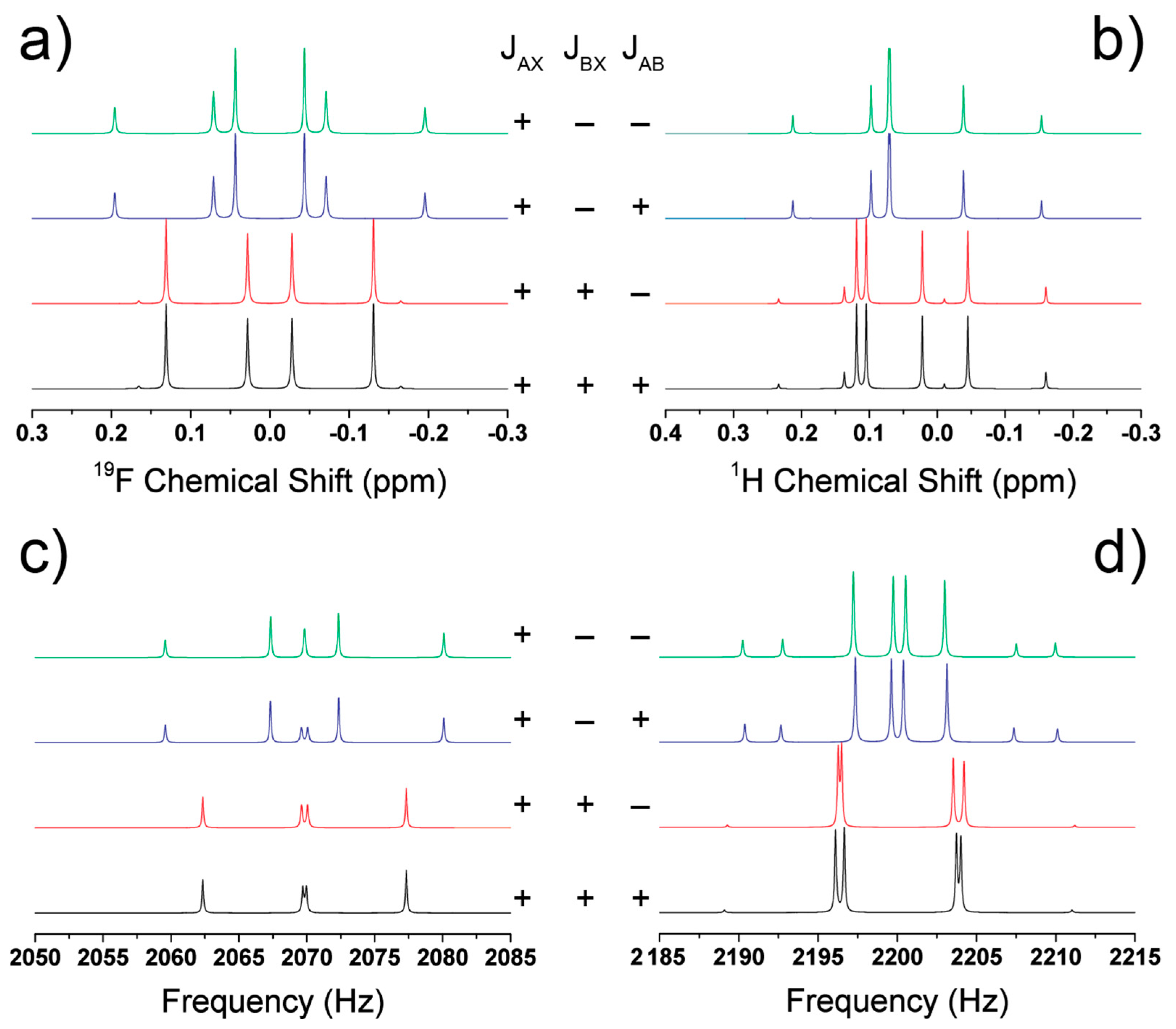
4.4. Determination of the Relative J-Coupling Signs

The J-couplings of 1,4-difluorobenzene are all positive, but for a majority of the fluorobenzenes, the simulated J-couplings had both positive and negative J-couplings. Traditionally, weakly coupled spin systems do not impart a sign dependence on the spectrum since the first order perturbation of the J-coupling results in equal splitting from the central frequency. However, in strongly coupled systems, the relative signs of the J-couplings are determinable. This has been mathematically developed for high field systems in which the difference in chemical shifts between two environments is on the order of the J-coupling, i.e., the strong homonuclear J-coupling limit [60,61,62,63,64,65,66]. The most simplistic of these systems is a strongly coupled AB system, in which A and B are homonuclei. In this case, A and B are both doublets and, as described by Hahn, the separation between the two middle lines will be [J² + (ν_A−ν_B)²]^0.5 − J, while the separation between the outer two lines is [J² + (ν_A−ν_B)²]^0.5 + J [67]. This is equivalent at LF to the relation developed for the strongly coupled heteronuclear S-I (AB system via Pople notation) system by Appelt et al. in which the four strong heteronuclear J-coupling transitions are given by [14]

$$v_1=v_I-\frac{J}{2}+\frac{J^2}{4\left({\nu }_I-{\nu }_s\right)},$$

(6)

$$v_2=v_I+\frac{J}{2}+\frac{J^2}{4\left({\nu }_I-{\nu }_s\right)},$$

(7)

$$v_3=v_s+\frac{J}{2}-\frac{J^2}{4\left({\nu }_I-{\nu }_s\right)},$$

(8)

$$v_4=v_s-\frac{J}{2}-\frac{J^2}{4\left({\nu }_I-{\nu }_s\right)},$$

(9)

The two inner lines are the ν₁ and ν₃ resonances, which are separated by

$$\left({\nu }_I-{\nu }_S\right)-J-\frac{J^2}{2\left({\nu }_I-{\nu }_S\right)},$$

(10)

while the two outer lines are separated by

$$\left({\nu }_I-{\nu }_S\right)+J+\frac{J^2}{2\left({\nu }_I-{\nu }_S\right)},$$

(11)

which is equivalent to the separation obtained by Hahn. Because the form of the Hamiltonian for J-coupling is the same for homonuclear or heteronuclear J-coupling, the consistency of peak spacing between strongly coupled two spin heteronuclear or homonuclear spins is expected. This gives additional credence to extending the Pople notation into the strong heteronuclear J-coupling regime, as the strongly coupled heteronuclear and strongly coupled homonuclear system two-spin systems AB and AX give the same analytical result for the transition frequencies. Therefore, the effects observed in the strong homonuclear case will extend into the strong heteronuclear regime. In the strong homonuclear J-coupling case, the next simplest system is the ABX system, in which two magnetically inequivalent, but strongly coupled protons, weakly couple to a heteronucleus, such as F. In this system, there are three J-couplings: J_AX, J_BX, and J_AB. This system has been treated by several authors and will not be fully presented here; only the pertinent aspects will be covered.

In this system, there are 14 observable transition frequencies [61], which all depend on the term C_m, given by

$$C_m=\frac{1}{2}\sqrt{{[\left({\nu }_A-{\nu }_B\right)+m\left(J_{AX}-J_{BX}\right)]}^2+J_{AB}^2}$$

(12)

Here, m is the sum of the spins of all X nuclei, and m can have values of ±1/2. In this system, only the relative signs of J_AX and J_BX can be established, since C_m depends on the value (J_AX−J_BX). On the other hand, the J_AB term is always squared and will have the same relation to J_AX and J_AB, regardless of the relative sign of J_AB. At LF, the same ABX system assumes one or both A and B are in the strongly coupled heteronuclear regime, which transforms into an equivalent ABC system. As was demonstrated by Alexander, the relative signs of the ABC system can be determined [63]. In this spin system, 15 transitions are theoretically observable, although only 12 to 14 are typically reported in the literature [63,64]. To illustrate this point, the JCS and high field spectra were simulated for the ABX (C) system in which spins AB were strongly coupled at high field and spins ABC were strongly coupled at LF (Figure 10). Each spectrum was simulated with three J-couplings (J_AB, J_AX, and J_BX), whose relative signs were changed between each simulation. There are four unique sign combinations for these systems. As Figure 10 demonstrates, at high field (Figure 10a,b), only the relative signs of J_AX and J_BX may be determined, as the black (+ + +) and red (+ + −) spectra are equivalent, as were the blue (+ − +) and green (+ − −) spectra. However, at LF (Figure 10c,d), all three signs may be determined, as each spectrum is distinct for each sign combination. Therefore, for the same molecule analyzed at high field and LF, the LF spectrum allows determination of the relative signs for all coupled nuclei as long as the total spin system contains more than two spins, whereas coupling sign determination at high field requires a strong homonuclear J-coupling.

This extends into larger systems as well, particularly those investigated here, which were 6-spin systems. With larger spin systems of coupled nuclei, the relative signs of the J-couplings are also determinable. For example, if we investigate the relative signs of 1,4-difluorobenzene, there are five J-couplings and 2⁵ or 32 possible sign combinations. However, half of the combinations were degenerate and had the same relative sign relation, resulting in 16 unique sign combinations. The 16 unique sign combinations are shown in Figure 11, along with corresponding R-factors for best fit with the experimentally determined spectra. Clearly the relative signs have a significant impact on the JCS, and must be chosen correctly to accurately simulate the JCS. The sign change of ⁴J_HH impacted the spectra the least; however, the difference caused by changing the sign clearly impacted the R-factor. It should be noted that, while the relative signs of these systems can be determined, the absolute signs are not established by the JCS.

4.5. General Trends in the J-Couplings of Fluorobenzenes

With experimental data and calculations in hand, the signs and magnitudes of fluorobenzene J-couplings may now be assessed. In general, the magnitude of the J-couplings followed |³J_ortho| > |⁴J_meta| > |⁵J_para| for H-H and H-F couplings, and |³J_ortho| > |⁵J_para| > |⁴J_meta| for F-F couplings. As first identified by Williams and Gutowski, the J-coupling magnitude is inherently tied to the bonding characteristics of the sigma and pi bonds, and their analysis correctly predicts the magnitudes of the H-H, H-F, and F-F couplings [68]. However, this analysis does not result in the correct assignments of the relative signs. In contrast, the JCS and ab initio calculations can determine the correct relative J-coupling signs, as shown in Table 2. Of note are the ⁴J_FF and ⁵J_HF couplings, which showed a mixed behavior of both positive and negative values. For ⁵J_HF, the change in magnitude and the eventual change in sign was due to the number of protons neighboring the F. As the number of protons increased, the ⁵J_HF coupling increased and eventually became positive proceeding from pentafluorobenzene (0 H neighboring, ⁵J_HF = −4.19 Hz) to monofluorobenzene (2 H neighboring, ⁵J_HF = +0.50 Hz). For ⁴J_FF, as the total number of F atoms increased, the J-coupling became smaller and negative. Pentafluorobenzene is interesting because it has three different ⁴J_FF with some J-couplings positive while others are negative. Clearly, the nature and position of the H and F atoms in the ring dramatically influences the sigma and pi bonds, which alter the sign and magnitude of ⁴J_FF. This is further supported by the values of ⁴J_FF for 1,3,5-trifluorobenzene (+5.8 Hz [69]), 1,2,3,4-tetrafluorobenzene (+2.56 Hz [70]), 1,3-difluorobenzene (+6.52 Hz), and pentafluorobenzene (+1.3 Hz).

4.6. LF and High Field Subspectra

JCS can also provide additional spectral details not captured in high field spectra. Consider the high field spectra of 1,2,4,5-tetrafluorobenzene, which consists of a relatively simple spectral pattern showing a triplet for ¹⁹F and a quintet for ¹H (Figure 12). A cursory analysis of the spectra would suggest there are four magnetically equivalent F atoms coupled to two magnetically equivalent H atoms with a J-coupling of +8.65 Hz. However, since the mixing coefficient of ³J_HF and ⁴J_HF is small, albeit non-negligible, this results in an “oversimplified” spectrum where the high field resonances appear at an averaged position for the two J-couplings [71]. JCS provides additional insight into this proposed phenomenon since the JCS of both the ¹⁹F and ¹H portions of the spectra have additional features that exclud the possibility of magnetic equivalence between the ¹⁹F and ¹H environments. At high field, these spectral features overlap, which results in a relatively featureless spectrum. Simulation of the high field spectra at 9.4 T, using the same J-couplings and chemical shifts used to fit the experimental JCS, clearly shows that there is a triplet in the ¹⁹F spectrum and a quintet in the ¹H spectrum. However, the simulated spectra are considerably narrower than the experimental spectra, causing additional features to emerge in the simulation of the ¹H spectrum. On the other hand, the relaxation rate required to fit the ¹⁹F spectrum was 10 times larger than the relaxation rate used to fit the LF spectra. This is likely due to different relaxation mechanisms, where the high field relaxation results from chemical shift anisotropy rather than dipolar relaxation, as observed in LF [11]. The increased linewidth at high field obscured any spectral fine structure from being observed. Therefore, the high field spectral features did not result from a small mixing coefficient, but rather from a complex splitting pattern caused by magnetically inequivalent nuclei where any fine structure is obscured by the linewidth of the spectrum. A similar argument can be made for 1,4-difluorobenzene, which had the same, albeit reversed, Pople notation as 1,2,4,5-tetrafluorobenzene. Previous reports measuring fluorobenzene spectra, notably monofluorobenzene and 1,4-difluorobenzene in the strong coupling regime, have lacked the spectral resolution and SNR to differentiate signals in the strong and weak heteronuclear J-coupling regimes [23,32]. However, as demonstrated in this study, the strong heteronuclear J-coupling regime can, in most cases, provide additional details about structures that are masked at high field.

4.7. Chemical Shift Resolution at LF

The chemical shift, which we have shown can be measured at LF, is one of the primary metrics that delineate different electronic environments in a sample. Therefore, in the event of a mixture of ¹⁹F containing compounds, the chemical shift could be used to differentiate between different molecules. The resolution (Res) of two peaks, assuming Gaussian line shapes, is defined as

$$Res=1.18\frac{v_1-v_2}{{FWHM}_1+{FWHM}_2}$$

(13)

where ν and FWHM are the measured frequency and the full width at half maximum of the peak, respectively. With Res = 0.2, two peaks, while overlapping, are still distinguishable. Assuming a conservative FWHM of 0.15, as demonstrated here for the fluorobenzene compounds, we could measure a frequency difference of 0.0508 Hz, which corresponds to a ¹⁹F chemical shift of 24.56 ppm. Previous LF studies have reported linewidths as narrow as 0.05 Hz for ¹³C-labeled methanol, with a Larmor frequency of ≈2060 Hz corresponding to ≈8 ppm at 20% resolution [15]. If peaks are fully resolved, (Res = 1), a chemical shift difference of 41 ppm is discernable. Measurable chemical shift differences theoretically break the chemical equivalence of homonuclei (and by extension their magnetic equivalence) and can create a JCS without the presence of a heteronucleus. Therefore, differentiating various electronic environments via the chemical shift is feasible at these magnetic fields, but will ultimately be tied to the inherent relaxation mechanisms governing the linewidths of the samples. This is an additional parameter that may be used to obtain structural information, particularly for those nuclei that have higher Larmor frequencies and high atomic numbers, such as Th, Xe, Pb, and Pt.

5. Conclusions

A series of fluorobenzene compounds were investigated in the strong heteronuclear J-coupling regime at a magnetic field of ≈51 µT. Using simultaneous excitation and detection of ¹⁹F and ¹H nuclei, the spectra were well simulated on the basis of J-couplings, chemical shift, and relaxation properties, and the resultant spectra were analyzed qualitatively and quantitatively. The JCS are quantitative, allowing for pseudo-empirical formulas or relative concentrations to be derived. Further, operation in the strong heteronuclear J-coupling regime allows for more complex spin systems to be developed since all spins are strongly coupled. Pople notation may be applied in the strong heteronuclear J-coupling regime, providing a basis for describing the symmetries of JCS spectra between different compounds. The result is a JCS containing heteronuclear and homonuclear J-coupling interactions, whose relative signs can be established with fewer spins than a strongly coupled homonuclear system. Homonuclear J-couplings are observed if at least one heteronuclear J-coupling breaks the magnetic equivalence of the nucleus being detected. Additionally, in multiple instances, the LF JCS provides a more detailed spectra than high field NMR and allows the JCS to access magnetically inequivalent spins in the system for structural analysis. Furthermore, for non-H nuclei, the chemical shift becomes an important parameter for accurate simulation of the JCS. As the magnetic field homogeneity of these LF systems improves, it is likely that chemical shift will also serve to break the chemical equivalence of homonuclei.

References

1. Jacobsen, N.E. NMR Spectroscopy Explained: Simplified Theory, Applications and Examples for Organic Chemistry and Structural Biology; John Wiley & Sons: Hoboken, NJ, USA, 2007; pp. 1–688. [Google Scholar]
2. Bakhmutov, V.I. Solid-State NMR in Materials Science: Principles and Applications; CRC Press: Boca Raton, FL, USA, 2011; pp. 1–288. [Google Scholar]
3. Zhu, G. (Ed.) NMR of Proteins and Small Biomolecules; Springer: Berlin/Heidelberg, Germany, 2012; Volume 326, pp. 1–246. [Google Scholar]
4. Abragam, A. The Principles of Nuclear Magnetism; Oxford University Press: Oxford, England, 1961; pp. 1–599. [Google Scholar]
5. Duer, M.J. Introduction to Solid-State NMR Spectroscopy; Blackwell Science Ltd: Malden, MA, USA, 2014; pp. 1–368. [Google Scholar]
6. Slichter, C.P. Principles of Magnetic Resonance; Springer: Berlin/Heidelberg, Germany, 1990; pp. 1–658. [Google Scholar]
7. Reisch, M. Helium shortage looms. Chem. Eng. News 2017, 95, 11. [Google Scholar]
8. Reisch, M. Helium shortages will persist. Chem. Eng. News 2019, 97, 38. [Google Scholar]
9. Singh, K.; Blümich, B. NMR spectroscopy with compact instruments. TrAC Trends Anal. Chem. 2016, 83, 12–26. [Google Scholar] [CrossRef]
10. Grootveld, M.; Percival, B.; Gibson, M.; Osman, Y.; Edgar, M.; Molinari, M.; Mather, M.L.; Casanova, F.; Wilson, P.B. Progress in low-field benchtop NMR spectroscopy in chemical and biochemical analysis. Anal. Chim. Acta 2019, 1067, 11–30. [Google Scholar] [CrossRef] [PubMed] [Green Version]
11. Murali, N.; Krishnan, V.V. A primer for nuclear magnetic relaxation in liquids. Concepts Magn. Reson. 2003, 17A, 86–116. [Google Scholar] [CrossRef]
12. Lustig, E.; Hansen, E.A.; Diehl, P.; Kellerhals, H. NMR Subspectral Analysis Applied to Polyfluorobenzenes C6HnF6−n. IV. 1,2,4-Trifluorobenzene. J. Chem. Phys. 1969, 51, 1839–1845. [Google Scholar] [CrossRef]
13. Adams, R.W. Pure Shift NMR Spectroscopy. Emagres 2014, 3, 295–309. [Google Scholar]
14. Appelt, S.; Häsing, F.W.; Sieling, U.; Gordji-Nejad, A.; Gloggler, S.; Blümich, B. Paths from weak to strong coupling in NMR. Phys. Rev. A 2010, 81, 023420. [Google Scholar] [CrossRef]
15. Appelt, S.; Häsing, F.W.; Kühn, H.; Blümich, B. Phenomena in J-coupled nuclear magnetic resonance spectroscopy in low magnetic fields. Phys. Rev. A 2007, 76. [Google Scholar] [CrossRef] [Green Version]
16. Appelt, S.; Häsing, F.W.; Kühn, H.; Sieling, U.; Blümich, B. Analysis of molecular structures by homo—And hetero-nuclear J-coupled NMR in ultra-low field. Chem. Phys. Lett. 2007, 440, 308–312. [Google Scholar] [CrossRef]
17. Appelt, S.; Kühn, H.; Häsing, F.W.; Blümich, B. Chemical analysis by ultrahigh-resolution nuclear magnetic resonance in the Earths magnetic field. Nat. Phys. 2006, 2, 105–109. [Google Scholar] [CrossRef] [Green Version]
18. Halse, M.E.; Callaghan, P.T. A dynamic nuclear polarization strategy for multi-dimensional Earth’s field NMR spectroscopy. J. Magn. Reson. 2008, 195, 162–168. [Google Scholar] [CrossRef] [PubMed]
19. Halse, M.E.; Callaghan, P.T.; Feland, B.C.; Wasylishen, R.E. Quantitative analysis of Earth’s field NMR spectra of strongly-coupled heteronuclear systems. J. Magn. Reson. 2009, 200, 88–94. [Google Scholar] [CrossRef] [PubMed]
20. Trahms, L.; Burghoff, M. NMR at very low fields. Magn. Reson. Imaging 2010, 28, 1244–1250. [Google Scholar] [CrossRef]
21. Burghoff, M.; Hartwig, S.; Trahms, L.; Bernarding, J. Nuclear magnetic resonance in the nanoTesla range. Appl. Phys. Lett. 2005, 87, 054103. [Google Scholar]
22. McDermott, R.; Trabesinger, A.H.; Muck, M.; Hahn, E.L.; Pines, A.; Clarke, J. Liquid-state NMR and scalar couplings in microtesla magnetic fields. Science 2002, 295, 2247. [Google Scholar] [CrossRef] [Green Version]
23. Robinson, J.N.; Coy, A.; Dykstra, R.; Eccles, C.D.; Hunter, M.W.; Callaghan, P.T. Two-dimensional NMR spectroscopy in Earth’s magnetic field. J. Magn. Reson. 2006, 182, 343–347. [Google Scholar] [CrossRef]
24. Shim, J.H.; Lee, S.J.; Hwang, S.M.; Yu, K.K.; Kim, K. Two-dimensional NMR spectroscopy of 13C methanol at less than 5 μT. J. Magn. Reson. 2014, 246, 4–8. [Google Scholar] [CrossRef]
25. Trabesinger, A.H.; McDermott, R.; Lee, S.; Mück, M.; Clarke, J.; Pines, A. SQUID-Detected Liquid State NMR in Microtesla Fields. J. Phys. Chem. A 2004, 108, 957–963. [Google Scholar] [CrossRef]
26. Béné, G.J. Nuclear magnetism of liquid systems in the earth field range. Phys. Rep. 1980, 58, 213–267. [Google Scholar] [CrossRef]
27. Bernarding, J.; Buntkowsky, G.; Macholl, S.; Hartwig, S.; Burghoff, M.; Trahms, L. J-Coupling Nuclear Magnetic Resonance Spectroscopy of Liquids in nT Fields. J. Am. Chem. Soc. 2006, 128, 714–715. [Google Scholar] [CrossRef] [PubMed]
28. Zhang, Y.; Qiu, L.; Krause, H.-J.; Hartwig, S.; Burghoff, M.; Trahms, L. Liquid state nuclear magnetic resonance at low fields using a nitrogen cooled superconducting quantum interference device. Appl. Phys. Lett. 2007, 90, 182503. [Google Scholar] [CrossRef] [Green Version]
29. Liao, S.; Chen, H.; Deng, Y.; Wang, M.; Chen, K.L.; Liu, C.W.; Liu, C.I.; Yang, H.; Horng, H.; Chieh, J.J.; et al. Microtesla NMR and High Resolution MR Imaging Using High- Tc SQUIDs. ITAS 2013, 23, 1602404. [Google Scholar]
30. Buckenmaier, K.; Rudolph, M.; Back, C.; Misztal, T.; Bommerich, U.; Fehling, P.; Koelle, D.; Kleiner, R.; Mayer, H.A.; Scheffler, K. SQUID-Based Detection of Ultra-Low-Field Multinuclear NMR of Substances Hyperpolarized Using Signal Amplification by Reversible Exchange. Sci. Rep. 2017, 7, 1–9. [Google Scholar] [CrossRef] [Green Version]
31. Buckenmaier, K.; Scheffler, K.; Plaumann, M.; Fehling, P.; Bernarding, J.; Rudolph, M.; Back, C.; Koelle, D.; Kleiner, R.; Hövener, J.-B.; et al. Multiple Quantum Coherences Hyperpolarized at Ultra-Low Fields. Chem. Phys. Chem. 2019, 20, 2823–2829. [Google Scholar] [CrossRef]
32. Qiu, L.; Zhang, Y.; Krause, H.-J.; Braginski, A.I.; Burghoff, M.; Trahms, L. Nuclear magnetic resonance in the earth’s magnetic field using a nitrogen-cooled superconducting quantum interference device. Appl. Phys. Lett. 2007, 91, 072505. [Google Scholar] [CrossRef] [Green Version]
33. Wang, N.; Jin, Y.; Li, S.; Ren, Y.; Tian, Y.; Chen, Y.; Li, J.; Chen, G.; Zheng, D. Detection of nuclear magnetic resonance in the microtesla range using a high Tcdc-SQUID. J. Phys. Conf. Ser. 2012, 400, 052041. [Google Scholar] [CrossRef] [Green Version]
34. Hamans, B.C.; Andreychenko, A.; Heerschap, A.; Wijmenga, S.S.; Tessari, M. NMR at earth’s magnetic field using para-hydrogen induced polarization. J. Magn. Reson. 2011, 212, 224–228. [Google Scholar] [CrossRef]
35. Qiu, L.-Q.; Liu, C.; Dong, H.; Xu, L.; Zhang, Y.; Krause, H.-J.; Xie, X.-M.; Offenhäusser, A. Time-Domain Frequency Correction Method for Averaging Low-Field NMR Signals Acquired in Urban Laboratory Environment. ChPhL 2012, 29, 107601. [Google Scholar] [CrossRef]
36. Bergstrom Mann, P.; Clark, S.; Cahill, S.T.; Campbell, C.D.; Harris, M.T.; Hibble, S.; To, T.; Worrall, A.; Stewart, M. Implementation of Earth’s Field NMR Spectroscopy in an Undergraduate Chemistry Laboratory. J. Chem. Educ. 2019, 96, 2326–2332. [Google Scholar] [CrossRef]
37. Liao, S.-H.; Yang, H.-C.; Horng, H.-E.; Yang, S.Y.; Chen, H.H.; Hwang, D.W.; Hwang, L.-P. Sensitive J-coupling spectroscopy using high—Tc superconducting quantum interference devices in magnetic fields as low as microteslas. Supercon. Sci. Technol. 2009, 22, 045008. [Google Scholar] [CrossRef] [Green Version]
38. Liao, S.-H.; Chen, M.-J.; Yang, H.-C.; Lee, S.-Y.; Chen, H.-H.; Horng, H.-E.; Yang, S.-Y. A study of J-coupling spectroscopy using the Earth’s field nuclear magnetic resonance inside a laboratory. Rev. Sci. Instrum. 2010, 81, 104104. [Google Scholar] [CrossRef] [PubMed]
39. Kang, C.S.; Kim, K.; Lee, S.-J.; Hwang, S.-m.; Kim, J.-M.; Yu, K.K.; Kwon, H.; Lee, S.K.; Lee, Y.-H. Application of the double relaxation oscillation superconducting quantum interference device sensor to micro-tesla 1 H nuclear magnetic resonance experiments. Appl. Phys. Lett. 2011, 110, 053906. [Google Scholar]
40. Bevilacqua, G.; Biancalana, V.; Baranga, A.B.-A.; Dancheva, Y.; Rossi, C. Microtesla NMR J-coupling spectroscopy with an unshielded atomic magnetometer. J. Magn. Reson. 2016, 263, 65–70. [Google Scholar] [CrossRef] [Green Version]
41. Chizhik, V.I.; Kupriyanov, P.A.; Mozzhukhin, G.V. NMR in Magnetic Field of the Earth: Pre-Polarization of Nuclei with Alternating Magnetic Field. Appl. Magn. Reson. 2014, 45, 641–651. [Google Scholar] [CrossRef]
42. Blanchard, J.W.; Budker, D. Zero- to Ultralow-Field NMR. eMagRes 2016, 5, 1395–1410. [Google Scholar]
43. Kaseman, D.C.; Magnelind, P.E.; Widgeon Paisner, S.; Yoder, J.L.; Alvarez, M.; Urbaitis, A.V.; Janicke, M.T.; Nath, P.; Espy, M.A.; Williams, R.F. Design and Implementation of a J-coupled Spectrometer for Multidimensional Structure and Relaxation Detection at Low Magnetic Fields. Rev. Sci. Instrum. 2020, 91, 054103. [Google Scholar] [CrossRef]
44. Edgar, M.; Zeinali, F.; Mojally, M.; Hughes, C.; Riaz, S.; Weaver, G.W. NMR spectral analysis of second-order 19F-19F, 19F-1H and 13C-19F coupling constants in pentafluorobenzene and tetrafluoro-4-(morpholino)pyridine using ANATOLIA. J. Fluor. Chem. 2019, 224, 35–44. [Google Scholar] [CrossRef]
45. Wray, V.; Ernst, L.; Lustig, E. The complete 13C 19F, and 1H spectral analysis of the fluorobenzenes C6HnF6−n. III. The remaining members of the series; INDO MO calculations of JFH, JFF, JCH, and JCF. J. Magn. Reson. 1977, 27, 1–21. [Google Scholar]
46. Gottlieb, H.E.; Kotlyar, V.; Nudelman, A. NMR chemical shifts of common laboratory solvents as trace impurities. J. Org. Chem. 1997, 62, 7512–7515. [Google Scholar] [CrossRef]
47. Zhao, Y.; Truhlar, D.G. The M06 suite of density functionals for main group thermochemistry, thermochemical kinetics, noncovalent interactions, excited states, and transition elements: Two new functionals and systematic testing of four M06-class functionals and 12 other functionals. Theor. Chem. Acc. 2008, 120, 215–241. [Google Scholar]
48. Frisch, M.J.; Trucks, G.W.; Schlegel, H.B.; Scuseria, G.E.; Robb, M.A.; Cheeseman, J.R.; Scalmani, G.; Barone, V.; Petersson, G.A.; Nakatsuji, H.; et al. Gaussian 16 Rev. A.03; Gaussian: Wallingford, CT, USA, 2016. [Google Scholar]
49. Deng, W.; Cheeseman, J.R.; Frisch, M.J. Calculation of Nuclear Spin−Spin Coupling Constants of Molecules with First and Second Row Atoms in Study of Basis Set Dependence. J. Chem. Theory Comput. 2006, 2, 1028–1037. [Google Scholar] [CrossRef] [PubMed]
50. Joyce, S.A.; Yates, J.R.; Pickard, C.J.; Mauri, F. A first principles theory of nuclear magnetic resonance J-coupling in solid-state systems. J. Chem. Phys. 2007, 127, 204107. [Google Scholar] [CrossRef] [PubMed] [Green Version]
51. Hogben, H.J.; Krzystyniak, M.; Charnock, G.T.P.; Hore, P.J.; Kuprov, I. Spinach—A software library for simulation of spin dynamics in large spin systems. J. Magn. Reson. 2011, 208, 179–194. [Google Scholar] [CrossRef]
52. Suntioinen, S.; Laatikainen, R. Solvent effects on the 1H-1H, 1H-19F and 19F-19F coupling constants of fluorobenzene and 1,2-difluorobenzene. Magn. Reson. Chem. 1992, 30, 415–419. [Google Scholar] [CrossRef]
53. Lawrenson, I.J. High-resolution fluorine magnetic resonance spectra of some pentafluorophenyl derivatives. J. Chem. Soc. 1965, 0, 1117–1120. [Google Scholar] [CrossRef]
54. Gil, S.; Espinosa, J.F.; Parella, T. IPAP–HSQMBC: Measurement of long-range heteronuclear coupling constants from spin-state selective multiplets. J. Magn. Reson. 2010, 207, 312–321. [Google Scholar] [CrossRef]
55. Gil, S.; Espinosa, J.F.; Parella, T. Accurate measurement of small heteronuclear coupling constants from pure-phase α/β HSQMBC cross-peaks. J. Magn. Reson. 2011, 213, 145–150. [Google Scholar] [CrossRef]
56. Saurí, J.; Nolis, P.; Parella, T. Efficient and fast sign-sensitive determination of heteronuclear coupling constants. J. Magn. Reson. 2013, 236, 66–69. [Google Scholar] [CrossRef]
57. Appelt, S.; Häsing, F.W.; Kühn, H.; Perlo, J.; Blümich, B. Mobile High Resolution Xenon Nuclear Magnetic Resonance Spectroscopy in the Earth’s Magnetic Field. Phys. Rev. Lett. 2005, 94, 197602. [Google Scholar] [CrossRef] [Green Version]
58. Katz, I.; Shtirberg, L.; Shakour, G.; Blank, A. Earth field NMR with chemical shift spectral resolution: Theory and proof of concept. J. Magn. Reson. 2012, 219, 13–24. [Google Scholar] [CrossRef] [PubMed]
59. Harris, R.K.; Becker, E.D.; Cabral De Menezes, S.M.; Granger, P.; Hoffman, R.E.; Zilm, K.W. Further conventions for NMR shielding and chemical shifts (IUPAC Recommendations 2008). eMagRes 2007, 33, 41–56. [Google Scholar]
60. Diehl, P.; Pople, J. The analysis of complex nuclear magnetic resonance spectra: II. Some further systems with one strong coupling constant. Mol. Phys. 1960, 3, 557–561. [Google Scholar] [CrossRef]
61. Pople, J.; Schaefer, T. The analysis of complex nuclear magnetic resonance spectra: I. Systems with one pair of strongly coupled nuclei. Mol. Phys. 1960, 3, 547–556. [Google Scholar] [CrossRef]
62. Alexander, S. Relative Signs of Spin-Spin Interactions in Nuclear Magnetic Resonance. J. Chem. Phys. 1958, 28, 358–359. [Google Scholar] [CrossRef]
63. Alexander, S. Relative Signs of Spin-Spin Interactions in Nuclear Magnetic Resonance. II. J. Chem. Phys. 1960, 32, 1700–1705. [Google Scholar] [CrossRef]
64. Fessenden, R.; Waugh, J. Strong Coupling in Nuclear Resonance Spectra. II. Field Dependence of Some Unsymmetrical Three-Spin Spectra. J. Chem. Phys. 1959, 31, 996–1001. [Google Scholar] [CrossRef]
65. Gutowsky, H.; Holm, C.; Saika, A.; Williams, G. Electron Coupling of Nuclear Spins. I. Proton and Fluorine Magnetic Resonance Spectra of Some Substituted Benzenes1,2. JPC 1957, 79, 4596–4605. [Google Scholar] [CrossRef]
66. Williams, G.; Gutowsky, H. Determination of the Signs of Nuclear Spin-Spin Indirect Coupling Constants. J. Chem. Phys. 1956, 25, 1288–1289. [Google Scholar] [CrossRef]
67. Hahn, E.; Maxwell, D. Spin echo measurements of nuclear spin coupling in molecules. Phys. Rev. 1952, 88, 1070. [Google Scholar] [CrossRef]
68. Williams, G.A.; Gutowsky, H.S. Electron Coupling of Nuclear Spins. II. Molecular Orbital Interpretation of Coupling Constants Observed in Fluorobenzenes. J. Chem. Phys. 1959, 30, 717–723. [Google Scholar] [CrossRef]
69. Wray, V.; Lincoln, D.N. The complete 13 C, 19 F and 1 H spectral analysis of the fluorobenzenes C6HnF6∼-n.I.1,3,5-trifluorobenzene. J. Magn. Reson. 1975, 18, 374–382. [Google Scholar]
70. Lustig, E.; Duy, N.; Diehl, P.; Kellerhals, H. NMR Subspectral Analysis Applied to Polyfluorobenzenes C6HnF6–n. II. 1,2,3,4-Tetrafluorobenzene. J. Chem. Phys. 1968, 48, 5001–5007. [Google Scholar] [CrossRef]
71. Paterson, W.G.; Wells, E.J. NMR spectrum of para-difluorobenzene. I. Mol. Spectrosc. 1964, 14, 101–111. [Google Scholar] [CrossRef]
Figure 1. Comparison of the 1H spectra for 1,4-difluorobenzene (a) and 1,2,4-trifluorobenzene (b) using a superconducting high magnetic field (9.4 T, black), a permanent high magnetic field (1.43 T, red), and permanent low field magnetic field (51.5 µT, blue). The high field spectra are plotted on a chemical shift axis (bottom scale) and the low field spectrum is plotted on a frequency axis (top scale). As the field is decreased, in the high field regime, there is significant overlap of the peaks, which becomes problematic when multiple chemical shifts are present (b). The low field NMR spectrum has additional peaks in the spectrum that are not captured by either high field spectrum, and also provides fewer overlapping resonances in the case of the 1,2,4-trifluorobenzene (b).
Applsci 10 03836 g001
Figure 2. Instrument response of the tuned circuit used for detection of the fluorobenzene compounds without a sample. The blue dotted line corresponds to the center frequency of the 1H nucleus, while the red dotted line denotes the 19F response. The 19F resonances are preferentially enhanced, relative to 1H by a factor of 1.52. The 60 Hz overtone noise spikes were omitted for clarity.
Applsci 10 03836 g002
Figure 3. The 1H region of the JCS for benzene (a), monofluorobenzene (b), 1,2-difluorobenzene (c), 1,3-difluorobenzene (d), 1,4-difluorobenzene (e), 1,2,4-trifluorobenzene (f), 1,2,4,5-tetrafluorobenzene (g), and pentafluorobenzene (h). The black lines are the experimentally measured spectra, the red lines are the simulated spectra, and the blue lines are the residuals between the experimental and simulated spectra. Each spectrum also has a scaling factor, which is denoted below the compound name, indicating the amount the experimental, simulated, and residuals that were multiplied such that the maximum peak intensities of the experimental spectra (ah) were equivalent.
Applsci 10 03836 g003
Figure 4. The 19F region of the JCS for hexafluorobenzene (a), monofluorobenzene (b), 1,2-difluorobenzene, 1,3-difluorobenzene (c), 1,4-difluorobenzene (d), 1,2,4-trifluorobenzene (e), 1,2,4,5-tetrafluorobenzene (g), and pentafluorobenzene (h). The black lines are the experimentally measured spectra, the red lines are the simulated spectra, and the blue lines are the residuals between the experimental and simulated spectra. Each spectrum also has a scaling factor, denoted below the compound name, that indicates the amount the experimental, simulated, and residual data was multiplied such that the maximum peak intensities of spectra (ah) were equivalent.
Applsci 10 03836 g004
Figure 5. Differences in the J-couplings between the JCS and the literature values reported in [44] and [45]. The symbols correspond to different compounds (● monofluorobenzene, + 1,2 difluorobenzene, × 1,3-difluorobenzene, ◇ 1,4- difluorobenzene, ▲ 1,2,4- trifluorobenzene, ■ 1,2,4,5-tetrafluorobenzene, and ⬟ and ⌂ for pentafluorobenzene). The values on the y-axis correspond to the coupled positions on the benzene ring.
Applsci 10 03836 g005
Figure 6. Comparison between experimentally determined and ab initio calculated 4JHH (a) and 5JHF (b). The symbols correspond to different compounds (● monofluorobenzene, + 1,2 difluorobenzene, × 1,3-difluorobenzene, ◇ for 1,4 difluorobenzene, ▲ 1,2,4- trifluorobenzene, ⬟ for pentafluorobenzene). A linear dependence was observed for both datasets, which indicates that the opposite relative sign obtained from ab initio calculations is due to the known scaling issues for these calculations. Therefore, when calculated or experimental J-couplings are near zero, a sign error may result; however, this is remedied by applying a linear correction factor.
Applsci 10 03836 g006
Figure 7. Impact of chemical shift on the simulated spectrum of a hexafluorobenzene + benzene mixture (1:1). The red spectrum is the simulated spectrum assuming 19F δiso = 0 ppm. The black spectrum is the experimentally acquired JCS, which was well fitted in simulations with a δiso = −163.2 ppm (Figure 3a). The hexafluorobenzene chemical shift at these microtesla (μT) fields is a discernable shift of approximately −0.34 Hz.
Applsci 10 03836 g007
Figure 8. The Pople notation for the fluorobenzene compounds studied here. For each compound, there are two different Pople notations—the top is the traditional Pople notation for a high field spectrum in the strong homonuclear J-coupling limit, while the bottom notation is the Pople notation for the same system at LF, in the strong heteronuclear J-coupling limit. Note that at LF, the Larmor frequency difference was such that none of the nuclei were well separated and must all be considered as a single system.
Applsci 10 03836 g008
Figure 9. The simulated (red) and experimental spectra (black) of the 19F (top) and 1H (bottom) regions of 1,4-difluorobenzene. From bottom to top, the simulated spectra each contained an additional J-coupling, which appears to the right of each spectrum. Clearly, the subspectra in the experimental spectrum are well simulated only when all heteronuclear and homonuclear J-couplings were included, as denoted by the R-factor, which is included to the left of each simulated spectrum.
Applsci 10 03836 g009
Figure 10. The 19F (a) and 1H (b) high field NMR spectra of an ABX system, with J-couplings JAX = 10 Hz, JBX = 5 Hz, and JAC = 7 Hz. Note that the spectra were invariant to the relative sign of JAB and only depended on the relative sign of JAX and JBX. In spectra (c) and (d), the same spin system was in the strong heteronuclear J-coupling limit, such that the ABX system became the ABC system. Unlike the ABX system, which only has two distinct spectra, the ABC system has four distinct spectra. Therefore, the relative signs of all three J-couplings may be determined for the ABC system. The absolute signs of the J-couplings are denoted between the spectra and are consistent between the high field and LF spectra with black (+ + +), red (+ + −), blue (+ − +), and green (+ − −).
Applsci 10 03836 g010
Figure 11. The 16 different possible sign permutations of the 5 J-couplings measured for the JCS of 1,4-difluorobenzene. The absolute signs are denoted between the 19F (left) and 1H spectra (right). The same spectra were obtained when there were degenerative, same relative sign combinations (e.g., + + + + + is equivalent to − − − − −). The signs from left to right correspond to absolute signs of 3JHF, 4JHF, 5JFF, 3JHH, and 4JHH, respectively.
Applsci 10 03836 g011
Figure 12. The experimental high field (9.4 T) NMR spectrum (black) and JCS (blue) of 1,2,4,5-tetrafluorobenzene for both the 19F (left) and 1H (right) portions of the spectra. The high field spectrum was simulated (red) using the same parameters obtained from the experimental JCS. Multiple peaks in the simulated subspectra in the 1H region indicated that the experimental subspectra information was likely hidden at this field due to line broadening. The 19F high field simulated spectrum showed no subspectra structure. Clearly, the JCS provides more detailed subspectra than either high field spectrum.
Applsci 10 03836 g012