Short-Term Spatio-Temporal Drought Forecasting Using Random Forests Model at New South Wales, Australia


1
Centre for Advanced Modelling and Geospatial Information Systems (CAMGIS), Faculty of Engineering and IT, University of Technology Sydney, Sydney, NSW 2007, Australia
2
Department of Energy and Mineral Resources Engineering, Sejong University, Choongmu-gwan, 209 Neungdong-ro, Gwangjin-gu, Seoul 05006, Korea
3
Department of Geology & Geophysics, College of Science, King Saud University, P.O. Box 2455, Riyadh 11451, Saudi Arabia
*
Author to whom correspondence should be addressed.
Appl. Sci. 2020, 10(12), 4254; https://doi.org/10.3390/app10124254
Submission received: 19 May 2020
/
Revised: 18 June 2020
/
Accepted: 19 June 2020
/
Published: 21 June 2020
(This article belongs to the Special Issue Machine Learning Techniques Applied to Geospatial Big Data)
Abstract
:Featured Application
Authors are encouraged to provide a concise description of the specific application or a potential application of the work. This section is not mandatory.
Abstract
Droughts can cause significant damage to agriculture and water resources, leading to severe economic losses and loss of life. One of the most important aspect is to develop effective tools to forecast drought events that could be helpful in mitigation strategies. The understanding of droughts has become more challenging because of the effect of climate change, urbanization and water management; therefore, the present study aims to forecast droughts by determining an appropriate index and analyzing its changes, using climate variables. The work was conducted in three different phases, first being the determination of Standard Precipitation Evaporation Index (SPEI), using global climatic dataset of Climate Research Unit (CRU) from 1901–2018. The indices are calculated at different monthly intervals which could depict short-term or long-term changes, and the index value represents different drought classes, ranging from extremely dry to extremely wet. However, the present study was focused only on forecasting at short-term scales for New South Wales (NSW) region of Australia and was conducted at two different time scales, one month and three months. The second phase involved dividing the data into three sample sizes, training (1901–2010), testing (2011–2015) and validation (2016–2018). Finally, a machine learning approach, Random Forest (RF), was used to train and test the data, using various climatic variables, e.g., rainfall, potential evapotranspiration, cloud cover, vapor pressure and temperature (maximum, minimum and mean). The final phase was to analyze the performance of the model based on statistical metrics and drought classes. Regarding this, the performance of the testing period was conducted by using statistical metrics, Coefficient of Determination (R2) and Root-Mean-Square-Error (RMSE) method. The performance of the model showed a considerably higher value of R2 for both the time scales. However, statistical metrics analyzes the variation between the predicted and observed index values, and it does not consider the drought classes. Therefore, the variation in predicted and observed SPEI values were analyzed based on different drought classes, which were validated by using the Receiver Operating Characteristic (ROC)-based Area under the Curve (AUC) approach. The results reveal that the classification of drought classes during the validation period had an AUC of 0.82 for SPEI 1 case and 0.84 for SPEI 3 case. The study depicts that the Random Forest model can perform both regression and classification analysis for drought studies in NSW. The work also suggests that the performance of any model for drought forecasting should not be limited only through statistical metrics, but also by examining the variation in terms of drought characteristics.
1. Introduction
Droughts can be categorized as one of the most devastating natural hazards, as they can affect regional, or even national, scales [1,2,3]. The challenges toward drought studies are enormous, primarily due to the unavailability of a fixed definition. Different researchers in their respective fields have defined droughts based on their own requirements [4,5]. As an example, the deficiency in rainfall could alarm a meteorologist; however, for a hydrologist, drought occurrence begins when there is a reduction in stream flow and similarly is the case for agricultural and socioeconomic fields [4,6]. Moreover, the effect of climate change and anthropogenic activities has led to the occurrence of more severe and extended drought periods [7]. The analysis of various drought aspects has seen tremendous progress with the use of different climatic [8], remote sensing dataset [9] and the inclusion of various variables [10], which could potentially lead to a better understanding of a particular drought type. However, accurate forecasting of droughts is still a challenge, and researchers are looking into different aspects which could reflect the ground reality [11].
Since defining a drought is important, indices were developed based on certain variables and their dependences for the drought type being analyzed [11,12]. These can provide a path toward understanding drought. Over the years, several drought indices have been developed, using different variables. Yihdego et al. [13] have provided a list of indices with their pros and cons. Of the several indices, one that is popular among researchers is the Standard Precipitation Evaporation Index (SPEI), developed by Vincente-Serrano et al. [14]. The use of SPEI over other used indices is due to its involvement of both rainfall and temperature as factors, unlike Standard Precipitation Index (SPI), which only uses precipitation data. The use of SPEI has been tested in various parts of the globe and for different drought studies [15]. The performance of SPEI over other prominent drought indices like SPI and Palmer Drought Severity Index (PDSI) has been widely tested for several parts of the world under different climatic regions, with contrasting results. For instance, Reference [16] recommended using SPI for humid regions and SPEI for arid regions for a study based in India, whereas Reference [17] suggested to use SPEI over SPI and PDSI to identify drought conditions based on the study conducted at a global scale. Moreover, the use of SPEI in identifying the drought regions during the recent mega-fires in Australia has been tested by Nolan et al. [18] and was found to be an effective indicator. The calculation of the index could involve either the use of ground-based data, which can suffer from inhomogeneity due to its sparse location, or satellite-based, data which covers a large area but with variable bias and gap of data due to cloud or satellite return frequency. Although ground-based data has its own benefits especially when understanding at local scale, satellite-based data can also provide similar or even better understanding of the variables when studying at the regional level, which is the case for droughts. The use of global climatological datasets for drought studies is on the rise, and among the various available datasets, the Climate Research Unit (CRU) dataset is quite popular, owing to its longer time scale and finer spatial resolution. Sun et al. [19] tested 30 different global climatological datasets, and their variation in precipitation values found that reanalysis climatic datasets have the most discrepancy compared to other models. Therefore, the present study uses the CRU dataset, and the various associated and derived climatological variables from 1901 to 2018, at a spatial resolution of 0.5° [20], with a temporal resolution of one month for drought index calculation and forecasting purposes.
The studies on drought can be varied, ranging from monitoring, mitigation studies like vulnerability, risk, time series modeling and forecasting [12]. However, the key aspect of drought which makes it different from other hazards is it takes time to reflect its effects on any economic or agricultural sector. Therefore, forecasting becomes an interesting prospect as a reliable model could help in mitigating some effects of the drought. For this purpose, various techniques have been applied, like physical [21], stochastic [22], probabilistic [23] and data-driven [11] ones. However, among these data-driven models involving machine learning (ML) algorithms are comparatively less computationally intensive and could provide sufficient understanding without the requirement of extensive dataset types. Although the forecasting capabilities of physical-based models are accurate for atmospheric factors like temperature, they are less accurate for essential drought affecting parameters like rainfall [24]. Moreover, physical models are difficult to implement, as they require various data types involving complex models and require intensive computation power [25]. ML-based models have been used for drought forecasting for different drought affected regions of the world. As an example, Rhee and Im [26] used decision trees, Random Forest and extremely randomized trees for meteorological drought forecasting for South Korea. Similarly, Park et al. [27] used Random Forest to forecast severe drought for Western Korea. Of the various ML models, Random Forests (RFs) have the capability to handle large datasets involving multiple features, as is the case for the present study. RF has shown significant advantage over other supervised learning methods as it has the ability to handle highly non-linearly correlated data, robustness to noise and opportunity for efficient parallel processing [28]. Furthermore, the RF model has other important features, like intrinsic feature selection step and prior application to classification problem, and it can reduce variable space by providing an importance value for every feature. The use of RF models has been extensively carried out for various natural hazard studies for both regression and classification purposes, such as landslide [25], floods [29], earthquakes [30] and soil erosion [31].
The occurrence of a drought initiates with the deficiency in rainfall and the change in global climatic variables has had a serious effect on drought severity and longevity. Therefore, researchers have started to focus on the use of climatic variables, which could provide a better idea about drought trends both in spatial and temporal context. Deo and Sahin [10] used climatic indices, along with sea surface temperatures (SSTs), as they trigger rainfall availability, to understand drought occurrences for the Eastern Australia region. Similarly, Mulualem and Liou [8] used hydro-meteorological, climate, sea surface temperatures and topographic variables to forecast drought for the Upper Blue Nile region of Ethiopia. The current work uses precipitation, potential evapotranspiration, vapor pressure, cloud cover and temperature (maximum, minimum and mean) variables for forecasting purposes. However, most of the studies in the literature [2,8,32] have not used cloud cover and vapor pressure as a variable for drought forecasting, even though it is very relevant for hydrological modeling and vegetation health. It is important to note that most of the studies are conducted based on ground-based data, and the availability of cloud cover variable can also be of concern. Moreover, the study has shown the importance of climatic indices and sea surface temperatures; however, the present study did not use such indices, and future works would involve these variables, which would help to provide a better understanding of the drought forecasting model and the important variables.
The understanding of the drought is based on classes, which indicate various drought levels ranging from extremely dry conditions to extremely wet conditions [14], in the case of meteorological and hydrological drought or extreme vegetation deficit to above-normal vegetation conditions for agricultural drought [33]. The comprehensive understanding of a data-driven model should be based on its ability to perform either regression or classification tasks, or both [34]. The classification capability of the ML-based models for drought classes has seen the use of models like Artificial Neural Networks [35] and decision trees [26]. Compared to other models, the use of RF-based drought class classification is comparatively less.
Therefore, the present study aims to fulfill several gaps present in the literature. One of those gaps is the use of a freely available climatological dataset for determination and forecasting of drought index at both spatial and temporal scales. Moreover, apart from the use of several key variables, the inclusion of vapor pressure and cloud cover as variables is important to understand its impact on drought occurrences and has been explored in the present study. Furthermore, the performance ability of RF model was also tested. In summary, the work involved forecasting of SPEI index for New South Wales region, using the dataset from 1901 to 2018. The data was divided into three time periods, involving the training period of the input data and the variables used from 1901 to 2010, and the data from 2011 to 2015 was used for testing. The testing period helped us to identify the forecasting capabilities of the model. Finally, the classification capabilities of the model into different drought classes was tested during the validation period (2016–2018), using the receiver-operating characteristic curve approach.
2. Study Area
Australia is one of the most drought-affected countries in the world and has seen major drought events. One of the most prominent drought-affected areas is New South Wales (NSW), which is situated in the eastern part of the country. The state has seen major drought events, like the Federation Drought (1895–1902), World War II Drought (1937–1945) and the recent Millennium Drought (2001–2010) and several other minor droughts. Figure 1 shows the location of NSW in Australia and the mean annual rainfall based on CRU TS dataset of the study area [20]. Wittwer [36] estimated the economic impact due to droughts from 2017 to 2019, and found that a total of $8.1 Billion was lost during this period. The recent bushfires in the region have been found to be further aggravated due to the combination of drought conditions, dry vegetation and rise in temperature [37].
In recent times, there has been a rise in the frequency of droughts, and they are expected to increase in the near future, primarily due to the increase in temperature and the decrease in rainfall [38,39]. Hennessy et al. [38] found that the average temperature of NSW has increased by 1.08 °C between 1950 and 2017. In terms of precipitation, Dey et al. [40] analyzed the changes and found that there has been a decrease in the rainfall since 1950. Such changes emphasize the need to include climatic drivers as variables for drought study, and the present study attempted to do so. The Bureau of Meteorology (BOM) of Australia considers a drought to be when precipitation is below the 10th percentile for a continuous period of three months or more [40]. By this definition, it becomes imperative to understand the effect of hydro-meteorological variables on drought occurrences.
3. Data Used and Methodology
The data used were from the freely available climatological dataset, CRU, which provides land-based observations from 1901 to 2018 [20]. The dataset is prepared at a resolution of 0.5° × 0.5° and covers the entire world, except for Antarctica; the format is netCDF (Network Common Data Form). The dataset is prepared by using an angular distance weighting interpolation technique, with no missing pixels [41]. The use of the CRU gridded dataset has been found to be a good representative of climatic conditions over dry regions [42]. The CRU dataset has three distinct variable types, which cumulate to ten variables and have been widely used for several applications for assessing climatic variability [43]. The present study uses three types of variables, (i) primary (mean temperature and precipitation); (ii) secondary (vapor pressure and cloud cover); and (iii) derived variables (potential evapotranspiration, maximum and minimum temperature). The potential evapotranspiration (PET) has been defined by using the Penman–Monteith technique [44]. Figure 2 depicts the annual variation of monthly rainfall and monthly mean temperature measures in NSW region for 1901–2018. The bottom and top of the rectangular boxes represent the 25th and 75th percentiles, respectively, with the horizontal thick lines in the boxes depicting median values (50th percentiles); the whiskers indicate 1.5 times the interquartile range with the points reflecting outliers [45]. The annual variation of rainfall and mean temperature across all the pixels for the NSW region are depicted in Figure 3. The present study uses the CRU dataset first to determine the SPEI index and thereafter uses all the variables mentioned above to be used as predictive factors to forecast SPEI index, using Random Forests.
3.1. Standard Precipitation Evaporation Index
The SPEI index is based on the determination of climatic water balance (CWB) approach, which uses rainfall and potential evapotranspiration (PET) as input values, wherein CWB is defined as follows:
where R is rainfall, and i is the month counter, which provides a measure of water surplus or deficit for a given month. The log-logistic probability density function was used to transform the CWB series to standardized units at different monthly scales (1 and 3 months). Thereafter, the log-logistic distribution was used to determine SPEI, by using the inverse normal function [15]. The use of PET methods also has a significant effect on the drought index calculation, and Penman–Monteith (PM) has been suggested to be performed [15]. In cases of data unavailability, Hargreaves method has also been suggested to be used for SPEI index calculation [15]. The detailed explanation about the calculation of SPEI index can be found in References [14,15,46]. This could be crucial, as a calculation of PET using PM via other climatological, reanalysis or ground-based datasets could prove to be difficult, and due care needs to be taken when defining drought. This could be achieved by statistically validating the historical drought events and its variation with the global drought-monitoring tool, like the SPEI database [15]. The methodology of the present study is depicted in Figure 4. The time series data for SPEI 1 and SPEI 3 for the two major droughts (World War II Drought (1937–1945) and the Millennium Drought (2001–2010)) are depicted in Figure 5a,b. As the figure represents, SPEI was able to successfully capture the historical major droughts and can be considered as a good index, with the ability to capture droughts. The variation in SPEI values depict various drought classes, as mentioned in Table 1 [8].
CWBi = Ri − PETi
3.2. Random Forests and Performance Analysis
The study of drought forecasting has seen the use of various ML-based models; however, the present study focusses only on Random Forest (RF), as its performance is similar to other supervised learning models, such as support vector machine or boosted regression trees [9,47]. However, the RF-model has been comparatively less tested, especially in Australia. Previous studies have used remote-sensing-based data to forecast drought, using neural networks and RF [48] for wheat belts in the region. The present study forecasts the drought index, using a climatological dataset for the entire NSW region, and is the first study of its kind. The RF model was proposed by Reference [49], an ensemble technique which reduces over-fitting and reduces the uncertainty, proving to be much better than single-tree-based techniques. The other benefit of using an RF model is its ability to handle large datasets; it is also highly interpretable, especially involving multiple features. It provides a reliable global estimate of variable importance and also determines the marginal effect of a predictor on response variable [50]. The model initiates by initially building a forest of decision trees utilizing the bootstrap technique, wherein every tree is created independently, based on a randomized subset of predictor variables [51]. The trees grow to a maximum size, without pruning, and thereby the output mean from all the multiple decision trees is the final result [52], achieving effective regression performance [27]. We used the scikit learn library to carry out the RF model [53]. There are two key things while running the model: first, understanding the right set of hyper parameters (number of decision trees and number of features under each tree), which would tune the parameters and evaluate the model for every combination. Although there are several parameter-tuning techniques, we have focused on the use of two most popular techniques, random search and grid search. As the name suggests, the random search technique uses random combinations of hyper parameters to find the optimal solution, whereas the grid search technique utilizes a grid approach through every combination of the hyper parameters. We tested both the approaches and found grid search to provide better results. The concerns regarding over-fitting were addressed by using a cross-validation approach under both the techniques. Thereafter, analyzing the relative importance of the variables and finding out the key variables affecting the regression model is the key to develop a reliable and interpretable model. The default feature importance in scikit-learn has a tendency to depict high importance of continuous features, and it sometimes can be biased. Therefore, to counter this, we used a drop-column feature importance technique, using rfpimp Python package (https://pypi.org/project/rfpimp/), which is based on the permutation importance strategy [54]. Although this package is resource-intensive, it proved to be most accurate feature importance.
The performance of the RF model was carried out by using Coefficient of Determination (R2) and Root-Mean-Square-Error (RMSE) method. R2 determines the fitness between the predicted and original values, whereas RMSE measures the variance of errors between the real and predicted values [55]. The formulae for both the statistical measures are:
where is the mean value; and are observed and forecasted values and N is the number of data points.
where SSE is the sum of squared errors. The higher the value of R2, the better the predictive capability of the model is, with 1 depicting an exact relationship between observed and predicted values [8]. This provides a basis for whether the model is fit to be used for prediction.
4. Results and Discussions
The SPEI index was computed by using the SPEI ‘R’ package developed by Reference [14], for the entire period of CRU dataset. The input SPEI files were further divided into training (1901–2010), testing (2011–2015) and validation (2016–2018) periods.
4.1. Training Period
The use of an RF model involved understanding the relative importance of the variables used for both time durations. The results reveal that rainfall was most important in both scenarios, followed by PET and vapor pressure. However, the relative importance could show different results if a different PET model was used to determine the SPEI index. Vapor pressure is an important parameter and has proved to be very significant, as compared to other variables, such as temperature [56] and soil moisture [57], especially toward vegetation health. The relative importance of the input variables shows cloud cover and vapor pressure were significant factors. Cloud cover is derived from the sunshine hours as a percentage value. It has been rarely considered as a variable, and few works have shown its importance in drought. As an example, Jimenez et al. [58], in their study on droughts in the Amazonia region, analyzed its importance and found it to be a significant factor, owing to the long-term land use, land-cover change and forest loss in the region. Similarly, vapor pressure has shown a strong correlation with the water transport process in various vegetation types. The NSW region has low vegetation cover compared to Amazonia, and hence vapor pressure or soil moisture may have a lower impact on the drought index prediction capability. Although SPEI is categorized as hydrological or meteorological drought only, its effect on agricultural drought would be more prominent. However, the present work shows that, for the NSW region, vapor pressure can also play a key role in drought occurrence, and therefore future works should also include this variable, irrespective of the drought type. Figure 6 depicts the relative importance of the variables under SPEI 1 and SPEI 3. The results show that rainfall is highest among all the variables for both time scales. When considering the various temperature factors, the minimum and mean temperature variables are higher for SPEI 3 scenarios; however, the maximum temperature is higher for the SPEI 1 case. This suggests that there have been several instances of heatwaves or short periods of high temperature which have led to short-term droughts. This is also evident from the fact that the influences of PET and vapor pressure are higher for the SPEI 1 case.
4.2. Testing Period
Further, the model was validated for the testing period, using statistical metrics. For this, we calculated the mean index value of all the pixels and examined the variation in terms of drought categories. The reason why we are using drought classes is that there are not enough drought periods during the testing period in order to understand the variation in other drought perspectives (like duration and intensity). This is crucial, as the variation provides confidence to further inspect the model at a spatial scale and also along different drought characteristics. The results (Figure 7a,b) show that the prediction capability of the model under both time periods is quite similar, with SPEI 3 being predicted slightly better than SPEI 1, with the values of R2 being 0.76 and 0.73, respectively. During this period, we evaluated the variation as per the drought class. For example, if the predicted SPEI value was found to be in the same drought class (Table 1), the results were considered to be satisfactory for that particular month. The results show that the observed SPEI 1 value had the most months under near-normal conditions (73%), i.e., values ranging from −0.99 to 0.99, followed by moderately dry (10%) and moderately wet (6.67%). In the case of predicted values, 43 of the 60 months depicted same drought class between the observed and predicted SPEI 1 values, while the remaining varied. Similarly, for SPEI 3, the near-normal conditions were observed for 78%, followed by severely wet (10%) and moderately dry (8.33%). However, when analyzing the variations between the classes, 45 months depicted the same drought classes between predicted and observed values. The results show that statistical metrics may not always prove to be a useful quantification approach, and therefore it is important to analyze in terms of drought characteristics. For instance, in the present study, we used drought classes, but others can use drought duration and similar classes, provided they have sufficient data to analyze the variation.
4.3. Validation Period
The analysis between the observed and predicted values during the validation period was conducted in two ways. First, we analyzed the spatial variation between the observed and predicted SPEI values during January–March (Figure 8a,b), and thereafter we examined the variation in terms of drought classes. For classification purposes, we undertook a binary classification technique, by dividing the pixels into either drought or no drought. For this, all the pixels having an SPEI value less than −1 were considered as drought pixels, and the remaining as non-drought pixels. The spatial variation between the observed and predicted SPEI 1 values shows that the variation in drought intensity is not significant; however, there are periods where the SPEI values depict different drought classes. Moreover, the predicted images generally show a greater number of drought pixels and a lower number of non-drought pixels compared to observed images. However, the more important thing here to note is that the clusters among them certainly remain in the same spatial domain. As an example, the observed SPEI 1 and 3 values for January 2017 have negative values toward the southeast part of the region, and the same can be seen in the case of predicted values, but the number of pixels is certainly high in the latter case. Such an observation can be made for other months, as well, for both SPEI 1 and 3 time scales. This can be considered as a good indicator of the model, but concerns regarding variation in drought class are certainly pertinent. For instance, the minimum observed SPEI 1 value during March 2018 falls under moderately dry conditions, whereas the predicted image shows the minimum value falling under severely dry conditions. Similar conditions can be found across other months, under both of the SPEI time scales.
The spatial variation among the observed and predicted SPEI values depicted two types of results. (i) Even though the variation between minimum and maximum index values in the observed and predicted images was underestimated or overestimated, the clusters generally remained the same, with the number of predicted pixels under negative SPEI values being more than the observed pixels. (ii) There were pixels which predicted different drought classes than the observed ones, thus making it imperative to understand how many pixels were correctly predicted under each drought class. Therefore, for this purpose, Receiver Operating Characteristic (ROC) analysis [59] was used. The accuracy of the model depends on the number of correctly predicted cells for a definite drought class. The ROC curve is drawn with sensitivity on the ordinate and specificity on the abscissa [60]. The sensitivity represents the true positive ratio (TPR), and specificity represents the true negative ratio (TNR), which can be determined as follows:
where TP is true positive, TN is true negative, FP is false positive and FN is false negative. TP and TN are the numbers of pixels that are correctly classified, whereas FP and FN are the numbers of pixels which were incorrectly classified. The area under the ROC curve (AUC) determines the model’s ability for classification purposes, with values less than or equal to 0.5 indicating no better than random chance [35]. The classification was based on the seven different drought classes. During the validation period, the pixels were mostly composed of near-normal conditions, with few periods of moderately dry and severely dry conditions under both time durations. In total, out of the 36 months of the validation period, almost 70% were near normal condition, 7% each for severely dry and wet conditions, 11% and 5% for moderately dry and wet conditions, respectively. The number of pixels in each drought class was calculated for every month and categorized as drought (SPEI < −1) or non-drought (SPEI > −1), based on SPEI values. The AUC value of SPEI 1 classification was found to be 0.82, whereas SPEI 3 was found to be 0.84, which can be considered as a good performance (Figure 9).
Sensitivity = TP/(TP + FN)
Specificity = TN/(FP + TN)
The variation suggests that there are several pixels which are just at the borderline of a certain drought class, so any overestimation leads the representation to a different class. As an example, the minimum observed SPEI 1 value for February 2017 was −1.99, which reflects severe drought conditions; however, the predicted SPEI 1 value for the same period was −2.14, which reflects extreme drought conditions. Similar observation can be found for January 2017, 2018 and also in March 2018, wherein some pixels with values between 0.96 and 0.99 were overestimated to more than 1, thereby depicting moderately wet conditions instead of near normal.
For SPEI 3, such an observation can be seen in the month of January 2016, in which the observed minimum index value was −0.95, meaning near-normal condition, but the predicted was found to be −1.09, which represents moderately dry conditions. Similar observation can be made in January 2018 and February 2018. However, in March 2018, the minimum index value was underestimated, as the observed minimum value was −2.06, whereas the predicted minimum value was −1.92, thereby representing extremely dry and severely dry conditions, respectively. Therefore, it can be said that, when analyzing at a pixel level, there are situations wherein the observed values are in proximity to the threshold of drought class and the predicted values can overestimate or underestimate it.
5. Conclusions
The present study was conducted with the aim of forecasting droughts and understanding the climatic variables affecting it for the NSW region of Australia. The work involved determination of the SPEI index and forecasting the index, using a machine learning approach, namely, Random Forests to one- and three-month lead times. The index was calculated by using rainfall and PET values collected from CRU dataset from 1901 to 2018, and the climatic variables included rainfall, PET, vapor pressure, cloud cover, mean, maximum and minimum temperature, also gathered from CRU. The understanding of the forecasting ability of RF was analyzed by dividing the input data into three: first used for training (1901–2010), then testing (2011–2015) and finally validation (2016–2018). For the testing period, mean SPEI values of all the observed and forecasted pixels were analyzed, using R2 and RMSE statistical metric. For the validation period, the aim was to understand the classification accuracy of the model as per the drought classes, which were analyzed by using ROC-based AUC curves. The results from the study could be used for other drought-based applications, like urban heat, agriculture and fire emergency preparedness. The conclusions from the study are as follows:
- The relative importance of the hydro-meteorological variables used to forecast drought index shows that, apart from rainfall, PET is the most significant factor, followed by vapor pressure and mean temperature.
- The model shows good forecasting capability, with R2 value being 0.73 and 0.76, respectively, for SPEI 1 and SPEI 3 scenarios. However, when analyzing the variation as per drought classes, SPEI 3 depicted a greater number of similar classes in accordance to SPEI 1, thus providing slightly better predicative capability of the model for the former case.
- The classification aspect of the model into different drought classes was analyzed during the validation period. The results show that the model was able to correctly classify 82% and 84% for SPEI 1 and SPEI 3 time periods, respectively.
The present study shows that the use of the Random Forest model has the ability to perform well for both regression and classification problems concerning drought at short-term time scales for the NSW region. However, a future study should test out other models, either single or hybrid, for both aspects at longer time scales and understanding the variation for different drought characteristics.
Author Contributions
Conceptualization, A.D. and B.P.; methodology and formal analysis, A.D.; data curation, A.D.; writing—original draft preparation, A.D.; writing—review and editing, B.P.; supervision, B.P.; funding—B.P. and A.M.A. All authors have read and agreed to the published version of the manuscript.
Funding
This research was supported by the Centre for Advanced Modelling and Geospatial Information Systems (CAMGIS), Faculty of Engineering and Information Technology, in the University of Technology Sydney (UTS). This research was also supported by Researchers Supporting Project number RSP-2020/14, King Saud University, Riyadh, Saudi Arabia.
Acknowledgments
The authors are thankful to the reviewers for reviewing and suggesting valuable modifications, which has helped in improving the quality of this paper.
Conflicts of Interest
The authors declare no conflict of interest.
References
- Christian-Smith, J.; Levy, M.C.; Gleick, P.H. Maladaptation to drought: A case report from California, USA. Sustain. Sci. 2015, 10, 491–501. [Google Scholar] [CrossRef]
- Mishra, A.K.; Singh, V.P. Drought modeling–A review. J. Hydrol. 2011, 403, 157–175. [Google Scholar] [CrossRef]
- Rajsekhar, D.; Singh, V.P.; Mishra, A.K. Integrated drought causality, hazard, and vulnerability assessment for future socioeconomic scenarios: An information theory perspective. J. Geophys. Res.-Atmos. 2015, 120, 6346–6378. [Google Scholar] [CrossRef]
- Van Loon, A.F. Hydrological drought explained. Wiley Interdiscip. Rev.: Water 2015, 2, 359–392. [Google Scholar] [CrossRef]
- Van Lanen, H.A.J.; Wanders, N.; Tallaksen, L.M.; Van Loon, A.F. Hydrological drought across the world: Impact of climate and physical catchment structure. Hydrol. Earth Syst. Sci. 2013, 17, 1715–1732. [Google Scholar] [CrossRef] [Green Version]
- Sohrabi, M.M.; Ryu, J.H.; Abatzoglou, J.; Tracy, J. Development of soil moisture drought index to characterize droughts. J. Hydrol. Eng. 2015, 20, 04015025. [Google Scholar] [CrossRef]
- Van Loon, A.F.; Gleeson, T.; Clark, J.; Van Dijk, A.I.; Stahl, K.; Hannaford, J.; Di Baldassarre, G.; Teuling, A.J.; Tallaksen, L.M.; Uijlenhoet, R. Drought in the Anthropocene. Nat. Geosci. 2016, 9, 89. [Google Scholar] [CrossRef] [Green Version]
- Mulualem, G.M.; Liou, Y.-A. Application of Artificial Neural Networks in Forecasting a Standardized Precipitation Evapotranspiration Index for the Upper Blue Nile Basin. Water 2020, 12, 643. [Google Scholar] [CrossRef] [Green Version]
- Park, S.; Im, J.; Jang, E.; Rhee, J. Drought assessment and monitoring through blending of multi-sensor indices using machine learning approaches for different climate regions. Agric. Meteorol. 2016, 216, 157–169. [Google Scholar] [CrossRef]
- Deo, R.C.; Şahin, M. Application of the artificial neural network model for prediction of monthly standardized precipitation and evapotranspiration index using hydrometeorological parameters and climate indices in eastern Australia. Atmos. Res. 2015, 161, 65–81. [Google Scholar] [CrossRef]
- Fung, K.; Huang, Y.; Koo, C.; Soh, Y. Drought forecasting: A review of modelling approaches 2007–2017. J. Water Clim. Chang. 2019. [Google Scholar] [CrossRef]
- Mishra, A.K.; Singh, V.P. A review of drought concepts. J. Hydrol. 2010, 391, 202–216. [Google Scholar] [CrossRef]
- Yihdego, Y.; Vaheddoost, B.; Al-Weshah, R.A. Drought indices and indicators revisited. Arab. J. Geosci. 2019, 12, 69. [Google Scholar] [CrossRef]
- Vicente-Serrano, S.M.; Beguería, S.; López-Moreno, J.I. A multiscalar drought index sensitive to global warming: The standardized precipitation evapotranspiration index. J. Clim. 2010, 23, 1696–1718. [Google Scholar] [CrossRef] [Green Version]
- Beguería, S.; Vicente-Serrano, S.M.; Reig, F.; Latorre, B. Standardized precipitation evapotranspiration index (SPEI) revisited: Parameter fitting, evapotranspiration models, tools, datasets and drought monitoring. Int. J. Climatol. 2014, 34, 3001–3023. [Google Scholar] [CrossRef] [Green Version]
- Pathak, A.A.; Dodamani, B.M. Comparison of Meteorological Drought Indices for Different Climatic Regions of an Indian River Basin. Asia-Pac. J. Atmos. Sci. 2019. [Google Scholar] [CrossRef]
- Vicente-Serrano, S.M.; Begueria, S.; Lorenzo-Lacruz, J.; Camarero, J.J.; Lopez-Moreno, J.I.; Azorin-Molina, C.; Revuelto, J.; Moran-Tejeda, E.; Sanchez-Lorenzo, A. Performance of Drought Indices for Ecological, Agricultural, and Hydrological Applications. Earth Interact. 2012, 16. [Google Scholar] [CrossRef] [Green Version]
- Nolan, R.H.; Boer, M.M.; Collins, L.; Resco de Dios, V.; Clarke, H.; Jenkins, M.; Kenny, B.; Bradstock, R.A. Causes and consequences of eastern Australia’s 2019-20 season of mega-fires. Glob. Chang. Biol. 2020. [Google Scholar] [CrossRef] [Green Version]
- Sun, Q.; Miao, C.; Duan, Q.; Ashouri, H.; Sorooshian, S.; Hsu, K.L. A review of global precipitation data sets: Data sources, estimation, and intercomparisons. Rev. Geophys. 2018, 56, 79–107. [Google Scholar] [CrossRef] [Green Version]
- Harris, I.; Osborn, T.J.; Jones, P.; Lister, D. Version 4 of the CRU TS monthly high-resolution gridded multivariate climate dataset. Sci. Data 2020, 7, 1–18. [Google Scholar] [CrossRef] [Green Version]
- Van Loon, A.; Van Huijgevoort, M.; Van Lanen, H. Evaluation of drought propagation in an ensemble mean of large-scale hydrological models. Hydrol. Earth Syst. Sci. 2012, 16, 4057–4078. [Google Scholar] [CrossRef] [Green Version]
- Han, P.; Wang, P.X.; Zhang, S.Y. Drought forecasting based on the remote sensing data using ARIMA models. Math. Comp. Model. 2010, 51, 1398–1403. [Google Scholar] [CrossRef]
- Hao, Z.; Hao, F.; Singh, V.P.; Sun, A.Y.; Xia, Y. Probabilistic prediction of hydrologic drought using a conditional probability approach based on the meta-Gaussian model. J. Hydrol. 2016, 542, 772–780. [Google Scholar] [CrossRef]
- Hudson, D.; Alves, O.; Hendon, H.H.; Marshall, A.G. Bridging the gap between weather and seasonal forecasting: Intraseasonal forecasting for Australia. Q. J. R. Meteorol. Soc. 2011, 137, 673–689. [Google Scholar] [CrossRef]
- Dikshit, A.; Sarkar, R.; Pradhan, B.; Segoni, S.; Alamri, A.M. Rainfall Induced Landslide Studies in Indian Himalayan Region: A Critical Review. Appl. Sci. 2020, 10, 2466. [Google Scholar] [CrossRef] [Green Version]
- Rhee, J.; Im, J. Meteorological drought forecasting for ungauged areas based on machine learning: Using long-range climate forecast and remote sensing data. Agric. For. Meteorol. 2017, 237, 105–122. [Google Scholar] [CrossRef]
- Park, H.; Kim, K. Prediction of severe drought area based on random forest: Using satellite image and topography data. Water 2019, 11, 705. [Google Scholar] [CrossRef] [Green Version]
- Fawagreh, K.; Gaber, M.M.; Elyan, E. Random forests: From early developments to recent advancements. Syst. Sci. Control Eng. Open Access J. 2014, 2, 602–609. [Google Scholar] [CrossRef] [Green Version]
- Chen, W.; Li, Y.; Xue, W.; Shahabi, H.; Li, S.; Hong, H.; Wang, X.; Bian, H.; Zhang, S.; Pradhan, B. Modeling flood susceptibility using data-driven approaches of naïve bayes tree, alternating decision tree, and random forest methods. Sci. Total Environ. 2020, 701, 134979. [Google Scholar] [CrossRef]
- Ji, M.; Liu, L.; Du, R.; Buchroithner, M.F. A comparative study of texture and convolutional neural network features for detecting collapsed buildings after earthquakes using pre-and post-event satellite imagery. Remote Sens. 2019, 11, 1202. [Google Scholar] [CrossRef] [Green Version]
- Arabameri, A.; Chen, W.; Blaschke, T.; Tiefenbacher, J.P.; Pradhan, B.; Tien Bui, D. Gully Head-Cut Distribution Modeling Using Machine Learning Methods—A Case Study of NW Iran. Water 2020, 12, 16. [Google Scholar] [CrossRef] [Green Version]
- Hao, Z.; Singh, V.P.; Xia, Y. Seasonal drought prediction: Advances, challenges, and future prospects. Rev. Geophys. 2018, 56, 108–141. [Google Scholar] [CrossRef] [Green Version]
- Meroni, M.; Fasbender, D.; Rembold, F.; Atzberger, C.; Klisch, A. Near real-time vegetation anomaly detection with MODIS NDVI: Timeliness vs. accuracy and effect of anomaly computation options. Remote Sens. Environ. 2019, 221, 508–521. [Google Scholar] [CrossRef] [PubMed]
- Reichstein, M.; Camps-Valls, G.; Stevens, B.; Jung, M.; Denzler, J.; Carvalhais, N. Deep learning and process understanding for data-driven Earth system science. Nature 2019, 566, 195–204. [Google Scholar] [CrossRef]
- Adede, C.; Oboko, R.; Wagacha, P.W.; Atzberger, C. A Mixed Model Approach to Vegetation Condition Prediction Using Artificial Neural Networks (ANN): Case of Kenya’s Operational Drought Monitoring. Remote Sens. 2019, 11, 1099. [Google Scholar] [CrossRef] [Green Version]
- Wittwer, G. Estimating the Regional Economic Impacts of the 2017 to 2019 Drought on NSW and the Rest of Australia; Victoria University, Centre of Policy Studies/IMPACT Centre: Budapest, Hungary, 2020. [Google Scholar]
- Steffen, W.; Hughes, L.; Mulling, G.; Bambrick, H.; Dean, A.; Rice, M. Dangerous Summer: Escalating Bushfire, Heat and Drought Risk; Climate Council of Australia: Potts Point, Australia, 2019. [Google Scholar]
- Hennessy, K.; Fawcett, R.; Kirono, D.; Mpelasoka, F.; Jones, D.; Bathols, J.; Whetton, P.; Stafford Smith, M.; Howden, M.; Mitchell, C. An Assessment of the Impact of Climate Change on the Nature and Frequency of Exceptional Climatic Events; CSIRO and Bureau of Meteorology: Canberra, Australia, 2008. [Google Scholar]
- Dikshit, A.; Pradhan, B.; Alamri, A.M. Temporal Hydrological Drought Index Forecasting for New South Wales, Australia Using Machine Learning Approaches. Atmosphere 2020, 11, 585. [Google Scholar] [CrossRef]
- Dey, R.; Lewis, S.C.; Arblaster, J.M.; Abram, N.J. A review of past and projected changes in Australia’s rainfall. Wiley Interdiscip. Rev. Clim. Chang. 2019, 10, e577. [Google Scholar] [CrossRef]
- Harris, I.; Jones, P.D.; Osborn, T.J.; Lister, D.H. Updated high-resolution grids of monthly climatic observations–the CRU TS3. 10 Dataset. Int. J. Climatol. 2014, 34, 623–642. [Google Scholar] [CrossRef] [Green Version]
- Miao, L.; Li, S.; Zhang, F.; Chen, T.; Shan, Y.; Zhang, Y. Future drought in the drylands of Asia under the 1.5 °C and 2.0 °C warming scenarios. Earth’s Future 2020. [Google Scholar] [CrossRef]
- Wang, J.; Yang, B.; Ljungqvist, F.C.; Zhao, Y. The relationship between the Atlantic Multidecadal Oscillation and temperature variability in China during the last millennium. J. Q. Sci. 2013, 28, 653–658. [Google Scholar] [CrossRef]
- Ekström, M.; Jones, P.; Fowler, H.; Lenderink, G.; Buishand, T.; Conway, D. Regional climate model data used within the SWURVE project? 1: Projected changes in seasonal patterns and estimation of PET. Hydrol. Earth Syst. Sci. 2007, 11, 1069–1083. [Google Scholar]
- Gariano, S.L.; Sarkar, R.; Dikshit, A.; Dorji, K.; Brunetti, M.T.; Peruccacci, S.; Melillo, M. Automatic calculation of rainfall thresholds for landslide occurrence in Chukha Dzongkhag, Bhutan. Bull. Eng. Geol. Environ. 2019, 78, 4325–4332. [Google Scholar] [CrossRef]
- Beguería, S.; Vicente-Serrano, S.M.; Angulo-Martínez, M. A multiscalar global drought dataset: The SPEIbase: A new gridded product for the analysis of drought variability and impacts. Bull. Am. Meteorol. Soc. 2010, 91, 1351–1356. [Google Scholar] [CrossRef] [Green Version]
- Naghibi, S.A.; Ahmadi, K.; Daneshi, A. Application of support vector machine, random forest, and genetic algorithm optimized random forest models in groundwater potential mapping. Water Resour. Manag. 2017, 31, 2761–2775. [Google Scholar] [CrossRef]
- Feng, P.; Wang, B.; Li Liu, D.; Yu, Q. Machine learning-based integration of remotely-sensed drought factors can improve the estimation of agricultural drought in South-Eastern Australia. Agric. Syst. 2019, 173, 303–316. [Google Scholar] [CrossRef]
- Breiman, L. Random forests. Mach. Learn. 2001, 45, 5–32. [Google Scholar] [CrossRef] [Green Version]
- Liaw, A.; Wiener, M. Classification and regression by randomForest. R News 2002, 2, 18–22. [Google Scholar]
- Heung, B.; Bulmer, C.E.; Schmidt, M.G. Predictive soil parent material mapping at a regional-scale: A random forest approach. Geoderma 2014, 214, 141–154. [Google Scholar] [CrossRef]
- Cutler, D.R.; Edwards, T.C., Jr.; Beard, K.H.; Cutler, A.; Hess, K.T.; Gibson, J.; Lawler, J.J. Random forests for classification in ecology. Ecology 2007, 88, 2783–2792. [Google Scholar] [CrossRef]
- Pedregosa, F.; Varoquaux, G.; Gramfort, A.; Michel, V.; Thirion, B.; Grisel, O.; Blondel, M.; Prettenhofer, P.; Weiss, R.; Dubourg, V. Scikit-learn: Machine learning in Python. J. Mach. Learn. Res. 2011, 12, 2825–2830. [Google Scholar]
- Parr, T.; Turgutlu, K.; Csiszar, C.; Howard, J. Beware Default Random Forest Importances. Available online: https://explained.ai/rf-importance/index.html (accessed on 10 May 2020).
- Paulescu, M.; Tulcan-Paulescu, E.; Stefu, N. A temperature-based model for global solar irradiance and its application to estimate daily irradiation values. Int. J. Energy Res. 2011, 35, 520–529. [Google Scholar] [CrossRef]
- Eamus, D.; Boulain, N.; Cleverly, J.; Breshears, D.D. Global change-type drought-induced tree mortality: Vapor pressure deficit is more important than temperature per se in causing decline in tree health. Ecol. Evol. 2013, 3, 2711–2729. [Google Scholar] [CrossRef] [PubMed]
- Novick, K.A.; Williams, C.A.; Phillips, R.; Oishi, A.C.; Sulman, B.N.; Bohrer, G.; Ficklin, D.L. Vapor pressure deficit is as important as soil moisture in determining limitations to evapotranspiration during drought. In Proceedings of the AGU Fall Meeting Abstracts, New Orleans, LA, USA, 11–15 December 2017. [Google Scholar]
- Jimenez, J.C.; Libonati, R.; Peres, L.F. Droughts over amazonia in 2005, 2010, and 2015: A cloud cover perspective. Front. Earth Sci. 2018, 6, 227. [Google Scholar] [CrossRef] [Green Version]
- Fawcett, T. An introduction to ROC analysis. Pattern Recognit. Lett. 2006, 27, 861–874. [Google Scholar] [CrossRef]
- Dikshit, A.; Sarkar, R.; Pradhan, B.; Jena, R.; Drukpa, D.; Alamri, A.M. Temporal Probability Assessment and Its Use in Landslide Susceptibility Mapping for Eastern Bhutan. Water 2020, 12, 267. [Google Scholar] [CrossRef] [Green Version]
Figure 1.
Study area in (a) Australia, and (b) mean annual rainfall of New South Wales (NSW) (1901–2018), based on Climate Research Unit Time Series (CRU-TS) dataset.
Figure 1.
Study area in (a) Australia, and (b) mean annual rainfall of New South Wales (NSW) (1901–2018), based on Climate Research Unit Time Series (CRU-TS) dataset.

Figure 2.
Box and plot chart of the annual variation of monthly rainfall and mean temperature values based on CRU TS dataset for the NSW, region from 1901 to 2018.
Figure 2.
Box and plot chart of the annual variation of monthly rainfall and mean temperature values based on CRU TS dataset for the NSW, region from 1901 to 2018.

Figure 3.
Variation of annual rainfall and mean temperature across the entire time duration (1901–2018) for the NSW region. The orange line represents the moving average of the past 20 years.
Figure 3.
Variation of annual rainfall and mean temperature across the entire time duration (1901–2018) for the NSW region. The orange line represents the moving average of the past 20 years.

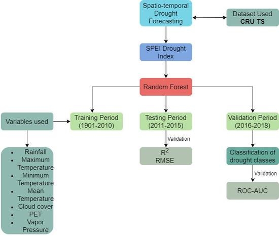
Figure 4.
Flowchart of the work being conducted.

Figure 5.
SPEI variation for two major droughts, (a) 1937–1945 (World War II Drought) and (b) 2001–2010 (Millennium Drought).
Figure 5.
SPEI variation for two major droughts, (a) 1937–1945 (World War II Drought) and (b) 2001–2010 (Millennium Drought).

Figure 6.
Relative importance of the variables for predicting SPEI 1 and SPEI 3 during training period.
Figure 6.
Relative importance of the variables for predicting SPEI 1 and SPEI 3 during training period.

Figure 7.
Variation between actual and predicted (a) SPEI 1 and (b) SPEI 3 values across all the pixels of the study region.
Figure 7.
Variation between actual and predicted (a) SPEI 1 and (b) SPEI 3 values across all the pixels of the study region.

Figure 8.
Spatial variation between observed and predicted (a) SPEI 1 and (b) SPEI 3 values during January–March (2016–2018).
Figure 8.
Spatial variation between observed and predicted (a) SPEI 1 and (b) SPEI 3 values during January–March (2016–2018).

Figure 9.
Receiver Operating Characteristic–Area under the Curve (ROC–AUC) curves of drought classification: (a) SPEI 1 and (b) SPEI 3 for the study region.
Figure 9.
Receiver Operating Characteristic–Area under the Curve (ROC–AUC) curves of drought classification: (a) SPEI 1 and (b) SPEI 3 for the study region.


Table 1.
Drought classification according to Standard Precipitation Evaporation Index (SPEI) index values.
Table 1.
Drought classification according to Standard Precipitation Evaporation Index (SPEI) index values.
| SPEI Values | Drought Classes |
|---|---|
| ≤−2.0 | Extremely Dry |
| −1.99 to −1.5 | Severely Dry |
| −1.49 to −1.0 | Moderately Dry |
| −0.99 to 0.99 | Near Normal |
| 1.0 to 1.49 | Moderately Wet |
| 1.5 to 1.99 | Severely Wet |
| ≥2.0 | Extremely Wet |
© 2020 by the authors. Licensee MDPI, Basel, Switzerland. This article is an open access article distributed under the terms and conditions of the Creative Commons Attribution (CC BY) license (http://creativecommons.org/licenses/by/4.0/).
Share and Cite
MDPI and ACS Style
Dikshit, A.; Pradhan, B.; Alamri, A.M. Short-Term Spatio-Temporal Drought Forecasting Using Random Forests Model at New South Wales, Australia. Appl. Sci. 2020, 10, 4254. https://doi.org/10.3390/app10124254
AMA Style
Dikshit A, Pradhan B, Alamri AM. Short-Term Spatio-Temporal Drought Forecasting Using Random Forests Model at New South Wales, Australia. Applied Sciences. 2020; 10(12):4254. https://doi.org/10.3390/app10124254
Chicago/Turabian StyleDikshit, Abhirup, Biswajeet Pradhan, and Abdullah M. Alamri. 2020. "Short-Term Spatio-Temporal Drought Forecasting Using Random Forests Model at New South Wales, Australia" Applied Sciences 10, no. 12: 4254. https://doi.org/10.3390/app10124254
Note that from the first issue of 2016, this journal uses article numbers instead of page numbers. See further details here.