Tridimensional Long-Term Finite Element Analysis of Reinforced Concrete Structures with Rate-Type Creep Approach


1
Department of Civil and Environmental Engineering, Politecnico di Milano, Piazza Leonardo da Vinci 32, 20133 Milan, Italy
2
Lombardi Ingegneria srl, Via Giotto 36, 20145 Milan, Italy
*
Author to whom correspondence should be addressed.
Appl. Sci. 2020, 10(14), 4772; https://doi.org/10.3390/app10144772
Submission received: 8 June 2020
/
Revised: 2 July 2020
/
Accepted: 9 July 2020
/
Published: 11 July 2020
(This article belongs to the Special Issue Recent Advances in Testing and Modelling Reinforced Concrete Structures)
Abstract
:This paper presents a general procedure for a rate-type creep analysis (based on the use of the continuous retardation spectrum) which avoids the need of recalculating the Kelvin chain stiffness elements at each time step. In this procedure are incorporated three different creep constitutive relations, two recommended by national codes such as the ACI (North-American) and EC2 (European) building codes and one by the RILEM research association. The approximate expressions of the different creep functions with the corresponding Dirichlet series are generated using the continuous retardation spectrum approach based on the Post–Widder formula. The proposed rate-type formulation is implemented into a 3D finite element code and applied to study the long-term deflections of a prestressed concrete bridge built in Romania, which crosses a wide artificial channel that connects the Danube river to the port of Constanta in the Black Sea.
1. Introduction
An accurate simulation of creep and shrinkage behavior is necessary for certain types of structures such as long-span prestressed box girders; cable-stayed or arch bridges; large bridges built sequentially in stages by joining parts; nuclear containments and vessels; large gravity, arch or buttress dams; cooling towers; large roof shells; and very tall buildings [1,2]. In this paper reference will be made to prestressed concrete beams, but the model developed is of general application.
Concrete creep can be modeled for service stress state levels (less than half of compressive strength) using the framework of linear visco-elasticity with aging [1]. As a consequence, the principle of superposition holds and the material behavior is uniquely described by a compliance or by a relaxation function. However, in practice, all the reinforced concrete design codes use the compliance (or creep) function to characterize the visco-elastic behavior, because the creep tests are much more common and easy to do than the relaxation tests. They usually describe the compliance function by a suitable formula with several parameters that can be calibrated by fitting experimental data or estimated using empirical formulae that take into account the concrete mix composition, curing conditions and time, member size and shape, and external relative humidity and temperature.
The compliance function expresses the evolution of uniaxial strain over time in a creep test for a unit uniaxial stress. This stress–strain relation can be written as
where is the aging creep function and the times t and correspond to the age of concrete starting from the initial setting time. However, the analytical evaluation of the integral in Equation (1) is possible only for simple models and simple stress histories. For general applications in finite element codes, the numerical integration of Equation (1) requires the storage of the entire stress history at each integration point of each finite element and, as a consequence, the evaluation of the integral requires an extensive memory allocation and an increasing number of calculations for each time step as the observation time t progresses. Several methods have been presented in the literature to simplify the calculation of creep strain under time history loading as in Equation (1), such as the effective modulus method [3], rate of creep method [4], the ageing coefficient method (AAEM method) [5] utilized in many applications, among others [6,7], the approach based on the aging linear viscoelastic theory [8], and, recently, the parallel creep method [9] that is extended in [10,11] for a general age-dependent constitutive law.
The computational cost of the integration of Equation (1) can be substantially reduced by replacing the integral stress–strain relation with a differential one (rate-type formulation, first proposed in [4]). This approach is based on the approximation of the compliance function by a Dirichlet series (i.e., a sum of exponentials) corresponding to a Kelvin rheological chain whose units are described by a differential equation that can be easily integrated in a step-by-step manner. This procedure transforms the original integral approach into a differential (rate-type) approach in which it is not necessary to store the entire load history but only a limited and fixed number of internal (history) variables. It also gives rise to a number of numerical calculations constant for each time step, independently of the length of the time interval considered.
In the rate-type approach the crucial point is the procedure adopted to convert the continuous creep function into its Dirichlet series approximation, due to the difficulties which arise in the identification of the series coefficients for aging formulations (typically used in codes and recommendations). One method was proposed in [12,13] for the study of the deflection behavior of the Koror-Babeldaob Bridge in Palau through a 3D finite element procedure. In their approach, to deal with the aging properties of the compliance function in each time step and at each integration point, use was made of the Widder’s formula to convert the aging compliance function into a continuous retardation spectrum for the current age of concrete. A discretization of the spectrum would then yield the current elastic moduli of the Kelvin units.
The purpose of this paper is to formulate a general procedure, also based on the use of the continuous retardation spectrum, capable of readily converting the integral creep problem into a rate-type one without the recalculation of the Kelvin chain stiffness elements at each time step. This procedure is then particularized with reference to three different creep constitutive relations, two important because recommended by professional associations in USA and Europe (ACI and CEB-Euro-Code) and one important for its diffusion in the research community, the RILEM B3 model.
The procedure has then been implemented in a three-dimensional finite element model for bridge design, capable of taking into account both the different shrinkage and drying creep properties of the various parts of the bridge cross-section and the shear lag effect, both of which cannot be captured by the classical beam theory commonly used in bridge design. In particular the shear lag effect influences drastically the accuracy of the calculation of the prestress loss and of the bridge deflection. As reported in [12,13] the shear lag occurs in different ways: In the transmission of vertical shear force due to vertical reaction at the pier and in the transmission of the concentrated forces of tendon anchors into the horizontal slabs and the vertical walls of the box.
In order to validate the proposed finite element formulation, two examples are considered, a prestressed simply supported beam and a prestressed cantilever box girder, for which the results of the 3D finite element analyses are compared with the one-dimensional calculations. Then the long-term behavior of a real bridge of “balanced cantilever girder” type, characterized by a central 155 m span, with two side symmetric 77.5 m spans, has been analyzed (and has been the motivation of this work). The bridge belongs to the new Medgidia-Constanta Motorway crossing a wide artificial channel that connects the Danube River to the port of Constanta in the Black Sea. It holds the record span-length in Romania for prestressed concrete deck type and has required for its construction concrete volumes of 14,700 m for foundations and 7700 m for piers and decks, total reinforcing steel weight of 2600 t, and total post-tensioning tendons weight of 390 t. For this bridge, the predictions of the various creep formulations in terms of deflections, prestress loss and stress state in the upper and lower slabs of the cross section are compared.
It must be remarked that an exact numerical analysis of this type of structures should be performed through a multi-physics time-dependent approach based on a hygro-thermo-chemical-mechanical model, as in [14,15,16], that could be useful in predicting the concrete time-dependent response. However, the multi-physics modeling is out of the scope of the manuscript and also the dimensions of this type of structures prevent its use for now. For general constitutive formulations that starts from early-ages, an interested reader can also refer to the formulations presented in [17,18,19,20,21].
2. Numerical Analysis of Creep Behavior
2.1. Integral Formulation
Using the principle of superposition and knowing the compliance function it is possible to determine the uniaxial strain evolution from any general uniaxial stress history, , in a integral-type form
where t is the current time, is the historic time and is the elapsed time and the integrals are understood in the Stieltjes sense, so that they can be evaluated even for discontinuous stress and strain evolutions. Equation (2) is the classical Volterra integral equation of creep that can be easily extended for multiaxial stress/strain considering that creep does not affect the Poisson’s ratio and, for this reason, it can be assumed as a constant. Under this assumption only the Young modulus is affected by creep and therefore Equation (2) can be extended for 3D general analysis as
where matrix is constant over time
The value will be used in all numerical simulations presented in this paper. Let us express Equation (2) in the incremental discrete form for finite element applications. In the time interval we can define the stress and strain increments:
Assuming a linear stress variation in the time interval, i.e., , we can rewrite Equation (7) as
where
To calculate the second expression in Equation (9) one needs to know the entire load history in each material point and in each time interval. This requires to store during the analysis a huge amount of information that increases drastically with the length of time interval considered. This makes the integral approach for creep prohibitive in a finite element program for long-term analysis, while it might be utilized for short-term processes such as early-age analyses, although this is not the most efficient procedure.
2.2. Rate-Type Creep Law
As a remedy, it was showed [1,22] that through the approximation of the creep function as a sum of negative exponentials (i.e., Dirichlet or Prony series) it is possible to convert the integral expression (in Equation (2)) into a set of linear differential equations, which turn out to be the governing equations of the well-known Kelvin chain rheological model with aging spring moduli and dashpot viscosities . These functions can be also identified as the coefficients of the Dirichlet series expansion of . Using this approach, a convenient approximation of the function can be written as
where are aging material parameters function of time being identified from the fitting of the given function at any given fixed . A simple and convenient choice for the other material parameters , called the retardation times, is to assume them constant. However, they must be chosen suitably with a not too large spacing in the log scale in order to approximate adequately the function in all time duration of interest during a the structural analysis. The function is the design compliance function being defined by some formula arising from the adopted code or standard. The term for instantaneous deformation can be considered included as the first term of the summation with a retardation time extremely small .
Substituting the approximation of the compliance function as in Equation (10) into the expressions in Equation (9) one gets
That can be rewritten as
where the integrals have been calculated using the mid point rule with and can be considered as internal variables that must be stored for the integration points of each finite element. Those internal variables can be updated according the following recurrence formula (obtained by calculating assuming a linear stress variation in the time step and constant time step increments )
It must be noted that the number of the internal variables for the rate-type formulation (Equations (8), (11), (13), and (14)) is now fixed and limited to N, in contrast to the integral formulation (Equations (8) and (9)) that requires the storage of the entire load history for each material point, which increases drastically with the final time of the analysis (for long-term behavior is typically many decades).
2.3. Aging Kelvin Chain
It is worth showing that the quasi-elastic constitutive law in Equations (8), (11), and (13) that has been just derived is fully equivalent to the solution of a rheological model consisting of a aging Kelvin chain with springs of stiffness in parallel with a dashpot with viscosities . To simplify the mathematical derivation, let us admit that in each time interval of the loading history the spring stiffnesses is constant and equal to where . Under this assumption the constitutive law of the aging Kelvin element in a time interval is given by the following first order differential equation
An effective numerical integration of Equation (15) can be done by virtue of the so-called exponential algorithm, which makes possible the use of increasing time steps with the same accuracy and numerical stability [1]. The exponential algorithm assumes that the stress varies linearly in the time interval so that the differential equation in (15) can be integrated exactly. The linear stress variation can be assumed as
where is the stress increment over the time step . With this stress variation the general solution of the differential equation in (15) can written as
The integration constants A and B of the particular integral can be obtained from the substitution of Equation (17) into (15) while C is calculated from the initial condition in each time step, . This yields the strain, , at the end the time step as
So the strain increment is
Considering now a rheological model chain of N Kelvin elements in series with a spring with stiffness , the total strain increment is given by
Substituting in this expression from Equation (19) and one gets the stress increment in the time step from to as
where
in which are the internal variables that can be updated according the recurrence formula in Equation (14).
Since and the two approaches are fully equivalent. This means that the approximation of an aging compliance function through a Dirichlet (or Prony) series transforms the classical Volterra integral equation of creep (Equation (2)) into a rate-type formulation governed by an aging Kelvin chain with spring moduli and viscosities obtained directly from the coefficient of the Dirichlet series approximation of the compliance function. At this point, to generalized the application of the rate-type approach, there is the need for a robust and reliable procedure capable of determining the coefficients of the Dirichlet series that approximate a given compliance function.
As pointed out in [23] the retardation times must be chosen “a priori” because their calculation from experimental data can give an ill-conditioned equation system. A suitable choice is
which means that the retardation times are equally spaced in a logarithmic scale and this gives smooth enough creep curves. Each of these times is representative of one order of magnitude, covering the interval from to . For a general analysis, 10 Kelvin units, i.e., , are enough to consider a wide spectrum time, i.e., from days to days.
2.4. Non-Aging Kelvin Chain
For non-aging material the expressions previously derived are simplified, since the equivalence is imposed with a non-aging Kelvin element (with spring stiffnesses constant). Moreover, the approximation of a non-aging compliance function, , through a Dirichlet (or Prony) series, is obtained using constant moduli as
The values of the coefficients can be determined by the best fitting a given non-aging compliance function either using a minimization algorithm (Least Squares or Levenberg– Marquardt algorithm) or passing through the continuous retardation spectrum [24], which is a more general approach that is summarized in the following.
As shown in Equation (24), a Kelvin chain model with N units gives a non-aging creep compliance function which can be approximated by a Dirichlet series as [22]
where , age of concrete, and age of concrete at the moment of loading. To deal with a general procedure and to avoid some weak points of other approaches [22,25], the continuous Kelvin chain model with infinite units (continuous spectrum), in which the retardation times are infinitely close, is used [24]. Passing through the continuous spectrum, the discrete spectrum can be obtained by discretizing the continuous one. The creep compliance function may be approximated in a continuous form as
where and is the continuous retardation spectrum, which has the same meaning in the logarithmic time scale as in the real time scale. Following the method developed by [26] and setting we have
and
The previous Equation (28) can be rewritten as
where if the Laplace transform of the function and is a constant. Using the inversion formula of Widder [27] the function can be obtained asymptotically as
where is the kth derivative of the function f. Remembering that and , we obtain the continuous retardation spectrum
The approximate spectrum of order k is obtained by assuming a finite value of k in Equation (31). For practical purpose an approximate spectrum of third order () may be used with enough accuracy [24,28], i.e.,
Decomposing the integral by a finite sum over finite time intervals given by Equation (23), the Equation (26) can be rewritten in the time of interest, i.e., , as
The integrals can be evaluated using the n-point Gaussian quadrature rule. Using the one-point quadrature rule in the intervals , which with Equation (23) are given by , the Equation (26) can be written as
and with the coefficients of the Dirichlet series given by
Comparing Equation (34) with Equation (24) we observe that the constant term must be added to and that .
However, as shown by Jirásek and Havlásek [28], the accuracy of the Dirichlet series which approximates a compliance function expressed by Equations (34) and (35) is not always good and it can often be substantially increased by appropriate modifications of the discrete retardation times adopted in the Dirichlet series. Jirásek and Havlásek [28] demonstrated that in many cases the accuracy of the Dirichlet series approximation cannot be increased by increasing the derivative order in Equation (32), but rather by the adjustment of the discrete retardation times, applied after the evaluation of the compliance coefficients. With this adjustment the Dirichlet series approximation is expressed as
The expressions of such adjustments, , are presented in the next section for each creep function considered in this study.
The presented approach for non-aging compliance function can be extended for aging creep function of the different codes and standards as it is presented in the next section.
2.5. Numerical Algorithm
As already reported in the literature [17,22,29,30], the finite element analysis of long term behavior with creep is much more efficient if a rate-type approach is used instead of an integral-type form. A Kelvin chain, as well as a Maxwell chain, arrangements of springs and dashpots can described the most general creep behavior [29,30]. Since the material constitutive law of concrete is typically based on the assumption of the strain additivity, a Kelvin chain is more convenient [16,31] than the Maxwell chain. Following the original idea of Bažant [32], the structural creep problem can be reduced to a sequence of elastic finite element analyses using an elastic stress–strain relation with inelastic strain, i.e, step-by-step linear elastic analysis for each time step. This means that in each time step the rheologic model can be considered non-aging and, consequently, its spring moduli and viscosity are constant and updated only at the beginning of the time step.
As shown in the previous section, the incremental quasi-elastic stress–strain relation suitable for a general finite element program can be written as (Equation (8) or Equation (21))
where and have been derived in the previous section (see Equations (11) and (13) or Equation (22)) and is the inelastic strain increment in each time step, such as the shrinkage strain or thermal strain [16]. This incremental stress–strain relation represent the quasi-elastic response of a non-aging kelvin chain that approximates a non-aging creep function .
The formula of the compliance functions generally adopted in standards or codes can be put in the form
where indicates the instantaneous elastic strain caused by a unit applied stress at the time and represents the creep deformation, which is expressed as the product of a constant , an aging term, , and a non-aging term, . The compliance function in Equation (38) can be approximated by the following Dirichlet series
where the coefficients are identified from the Dirichelt approximation of using the expression in Equation (35). In this case, the general incremental quasi-elastic stress–strain relation is still given by Equation (37) with the following expression for and
where can be taken as the time at the middle of the time step, . When a specific creep formulation is considered, from the expression of the coefficients must be calculated first and then, using the specified expressions for , , and , one can calculate the value of and to be utilized in the constitutive law of Equation (37). The formulation proposed for the rate-type creep analysis is based on the continuous retardation spectrum of the adopted constitutive relation for the compliance function. This spectrum is derived below for the most significant creep models.
3. Spectra Determination for Various Models
3.1. EuroCode 2 Model
The EuroCode 2 (EC2) expresses the creep behavior through the creep coefficient, , so that the compliance function may be expressed as
where is the modulus of elasticity at loading age . Comparing the compliance function in Equation (38) to the expression in Equation (42), we have
Considering the EuroCode 2 formulation reported in Appendix A, the previous expressions in Equation (43) can be rewritten as
The approximate continuum retardation spectrum of third order ( in Equation (31)) is given by
with for . The optimum adjustment factors, , in Equation (36) for the best approximation of the EC2 creep function are given by
3.2. ACI Model
According to the ACI-209R-92 code provisions, the compliance function is expressed as
where is the modulus of elasticity at loading age and the creep coefficient is given in Equation (A25). Comparing the compliance functions in Equation (38) to the one in Equation (48), we have
Recalling the ACI-209R-82 formulation, reported in Appendix B, the previous expressions in Equation (49) can be written as
The approximate continuum retardation spectrum of third order ( in Equation (31)) is given by
with for and . The optimum adjustment factors, , in Equation (36) for the best approximation of the ACI creep function are given by
The approximations of the ACI compliance function by Dirichlet series for different are compared with the exact function in Figure 2a with and . The maximum relative error, which is plotted in Figure 2b, is less than 1% providing a very good approximation of the ACI creep function.
The inelastic strain incremental for the ACI model due to shrinkage in each time step is given by
where the formula of can be found in Equation (A20).
3.3. B3 Model (RILEM)
According to the B3 model developed by Bažant and coworkers at Northwestern University [33] and recommended by RILEM, the compliance function (Equation (A34) of Appendix C) is expressed as
Since the term needs a specific different calculation respect to the previous formulations, it does not appear in Equation (55). Recalling the B3 formulation, reported in Appendix C, the previous expressions in Equations (55) and (54) can be written as
The function describes basic creep by a log-power law with aging incorporated through the solidification theory [22,34] with an additional logarithmic term that reflects viscous flow. This term can be described by a dashpot with age-dependent viscosity and can be treated directly in the rate form, without the need to construct a Dirichlet series approximating its compliance function. Therefore, to describe the basic creep of B3 model, only the spectrum of the log-power is needed. Its third order approximation ( in Equation (31)) with the continuous retardation spectrum (Equation (32)) is given by
with (from Equation (35)) for days. The quality of the approximation of the B3 compliance function by Dirichlet series with the coefficient obtained from Equation (58) is shown in Figure 3a for different and with . The approximated curves exhibit a maximum error, plotted in Figure 3b, below 1% with the adjustment factors for and . For the numerical calculation of the basic creep function of the B3 model, in Equation (56), reference must be made to the solidification theory [22,34] for which the visco-elastic strain rate is given by
Substituting in the second expression of Equation (59) the Dirichlet approximation of the compliance function, , expressed through the coefficient given by Equation (58) we have
where the are now the internal variables that can be calculated with the following recursive formula, obtained by evaluating with the second expression in Equation (60) and assuming a linear variation of the stress increment in the time step from to
Rewriting the first expression of Equation (59) in discrete form, , and substituting the obtained from Equations (61) and (60), one gets the contribution of the basic creep, , which must be added to the stress–strain relations in Section 2.5, in the following form
where , are the internal variable obtained from Equation (61), and the last term represents an additional logarithmic term that reflects the purely viscous flow. Those two terms in Equations (62) and (63) must be added to the expression in Equations (40) and (41), respectively.
In addition to the basic creep, in the model B3 there is a separate drying creep term (see Equation (A37)), which is capable of reproducing the Pickett effect. Like the shrinkage, the drying creep term is bounded and depends on the humidity and the cross section thickness. Without losing generality we assume (otherwise a constant term should be added to the compliance function) and comparing the compliance function in Equation (38) to the expression of B3 drying creep compliance we have
The approximate third order continuum retardation spectrum of this drying creep function can be expressed as
where , , , , and (from Equation (35) with days, , and ). The reliability of the approximation of the B3 drying compliance function by Dirichlet series with the coefficient obtained from Equation (65) is shown in Figure 3c for different and with , , and . The approximated curves in the figure exhibit a maximum error below 2% as showed in Figure 3d. To have that lever of error (certainly admissible for practical applications) the terms of the Dirichlet series are increased up to 13, with a denser set of retardation times with retardation time interval of . The Dirichlet approximation of the B3 drying creep function reads
where , with days, from Equation (65), and with , i.e., drying and loading act simultaneously at time , and .
4. Numerical Validation of the Finite Element Model
In this section two numerical applications of the proposed approach are presented. The previously illustrated constitutive relations have been implemented in three-dimensional finite element program, because only this approach can easily analyze cases with complicated loading history, with different distribution in the structure of the material properties, with different construction phases, with cross-section in which the inhomogeneous effects of the diffusion processes are not negligible, with changes of the structural configuration, and with the shear-lag effect. This effect is characterized by out-of-plane warping of cross-sections where there is high shear force and by a nonlinear stress distribution, that are neglected by the classical beam-type analysis. The reason for taking it into account is that the shear lag due to the self weight is stronger than the one generated by the prestress and since the total deflection is a small difference of the downward deflection due to self-weight and the the upward deflection due to prestress, a small error in only one contribution produces a larger error in the total deflection. The finite element program employed for all the numerical simulations presented in this work is a Fortran code written by the first author in which the implicit time (real time) integration is performed using the Newton–Raphson method with a constant global stiffness matrix obtained with the value of the Young modulus at 28 days.
All the calculations and the numerical simulations are done assuming concrete in the uncracked stage, which can be justified by the limited tensile stresses in concrete. However, the proposed formulation can be easily extended to include non-linear behavior and cracking, for instance see [13,16,30,35] for mesoscale formulation. Moreover, the relaxation of the steel prestress bars or strands is not considered in the analyses which follow.
4.1. Numerical Simulation of a Prestressed Beam with I-Shaped Solid Cross-Section
The first example concerns a simply supported prestressed concrete beam with a constant I-shaped cross-section and with a single equivalent prestressing strand with steel diameter of 36 mm. The cross-section geometry of the considered beam is showed in Figure 4a, the boundary and loading conditions in Figure 4b. In order to validate the numerical formulation of the rate type creep model and its implementation into a three-dimensional finite element code, the mid-span deflection in time obtained from the finite element analysis is compared with its analytical calculation resulting from the Effective Modulus Method (EMM) [36] applied to the type of load history considered (see Figure 4c). Using the EMM the mid-span deflection can be calculated with the Principle of Virtual Work as
where is the effective modulus calculated from the creep function , is the effective shear modulus, is the cross-section moment of inertia, is the cross-section area, and is the shear factor [37]. The geometric properties depend on time through the homogenization coefficient . Assuming a constant cross-section and substituting the bending moment and the shear corresponding to the external uniform distributed load of 30 kN/m applied at time (sketched in Figure 4c) the mid-span deflection, , is given by
The prestressing tendon is modeled using beam finite elements connected rigidly to the nodes of the three-dimensional mesh (no slip). No regular reinforcing steel bars are considered in this application. The prestress force, , is applied in the tendon by assigning an initial equivalent thermal deformation which generates a stress which accounts for the initial elastic loss. The initial prestress force is of 1297 kN that is equal to prestressing force of kN after the initial elastic loss. Substituting the bending moment ( with the eccentricity of the tendon) the mid-span deflection, , is given by
It has been considered no relaxation of the steel and no shrinkage of concrete in this first example. The creep model adopted is the EC2 creep model assuming , m m mm, MPa, MPa, = 14 days. The comparison between the mid-span deflection of the beam as calculated using the beam theory with the EMM (Equations (69) and (70)) and the deflection obtained with the 3D finite element analysis with rate type formulation is presented in Figure 5 for different loading conditions showing a coincidence of the calculated deflections with the two methods. The excellent agreement is also conformed by the evolution of the normal stresses and by the force in the steel tendon, as shown in the following.
The normal stresses in the concrete cross-section can be calculated as
in which y is the distance from the centroid of the homogenized section and M is the bending moment. In the following, tensile stresses are considered positive. The force in the prestress steel tendon is also compared in Figure 6a with the analytical value that can be calculated using the age-adjusted effective modulus approach, given by
where is the age-adjusted effective modulus with , is the stress in concrete at the level of the tendon and is its variation in time, calculated using Equation (71) with the appropriate y. Usually, in the design procedure and also in the code recommendations, only the first term in Equation (72) is considered. In Figure 6a the variation in time of the force in the steel tendon is shown and compared with the analytical solution obtained from Equation (72) presenting a perfect agreement between them. Figure 6b–d display the evolution of the normal stresses obtained with the analytical (Equation (71)) and the numerical solution, again the results pretty much coincide.
In addition also the capability of the proposed approach for complex load histories is considered. Complex load histories that are reported on the left of Figure 7 are adopted and the corresponding numerical solution is compared with the exact integral formula
In addition in Figure 7 is also reported the approximate solution give by the AAEM
4.2. Numerical Simulation of a Prestressed Box Girder
The second example deals with a cantilever prestressed concrete box girder with variable cross-section and with two equivalent prestressing bars with steel diameter of 36 mm. In Figure 8a,b are shown the cross-section geometries at the fixed and at the free end, respectively, of the considered girder. The boundary and loading conditions are presented in Figure 8c. For this type of geometry, the drying process, which drives shrinkage and drying creep, causes nonhomogeneity of shrinkage and creep properties throughout the cross-section that are nonsymmetric with respect to neutral axis. This phenomenon can not be captured by a 1D beam analysis and it has often been one major cause of gross mispredictions of long-time deflections of structures [38,39]. Therefore, only using a 3D analysis one can capture the different properties in the cross-section.
Moreover, for this application, the 3D finite element numerical solution of the rate type creep model is compared with the analytical calculation using the beam theory (with the above-mentioned limitations) and the Effective Modulus Method (EMM) using the load history plotted in Figure 8c). Using the EMM the free end displacement can be easily calculated with the Principle of Virtual Work as in Equation (68) where the effective modulus and effective shear modulus are calculated as in previous example. The moment of inertia, , the area, , and the shear factor, , are calculated according to the current the cross-section, which varies from the cross-section at the fixed end in Figure 8a to the cross-section at the free end. No relaxation of the steel and no shrinkage of concrete is adopted for this second example. The creep model adopted is the EC2 creep model assuming , MPa, MPa, = 14 days, and a cross-section value of which is assumed varying lineally from 218.6 mm at the fixed end to 155.56 mm at the free end. The comparison between the displacements of the beam as calculated using the beam theory with the EMM (Equations (69) and (70)) and the displacements obtained with the 3D finite element analysis with rate type formulation is presented in Figure 9 for different loading conditions showing a perfect coincidence of the calculated deflections with the two methods. The excellent agreement is also confirmed by the evolution of the normal stresses and by the force in the steel tendon. The normal stresses in the concrete cross-section can be calculated using the expression in Equation (71) with the correction factors proposed by [40] as and for the straight and tapered side, respectively. In Figure 10a the time evolution of the axial force in the steel tendon is shown and compared with the analytical solution obtained from Equation (72) presenting a very good agreement between them. Figure 10b–d report the evolution of the normal stresses obtained with the analytical (Equation (71) with the above correction factors) and the numerical solution which basically correspond with each other.
5. Numerical Simulation of the Long-Term Behavior of a Bridge
The bridge is of the “balanced cantilever girder” type, built with segments cast from piers with mobile equipment, and it is characterized by a central 155 m span (the longest span in Romania for prestressed concrete box girder bridges), with two side symmetric spans of 77.5 m (see Figure 11). The deck has a varying depth provided by a curved soffit of parabolic shape. The depth of cross section varies from maximum value of 10 m at the pier axis, to a minimum value of 2.4 m, at mid span and at the abutment supports. The upper slab is 14.75 m wide and transversally inclined of 2.5% (see Figure 12).
The layout of the post tensioned internal tendons (total length 10 km/single deck), follows the upper and lower slabs (see Figure 12). The upper tendons counterbalance the action of the free cantilever under gravity loads. The lower tendons are located along bottom slab and anchored to reinforced concrete internal blisters. The layout is symmetric with respect to the midlength of the central span both for the central and the side spans.
The bridge deck is supported by two piers and two abutments through two seismic bearings at each support. The bearings are of the “friction pendulum” type, which develop friction forces both in static conditions, due to static forces and small displacements, and dynamic condition providing dissipation. Under seismic loads (moderate for that construction site) the whole concrete structure develops only elastic behavior, because dissipation and lengthening of the natural period of the structure are provided by the seismic bearings.
Piers 1 and 2 are characterized by same shape but different height, respectively, 17.4 m and 16.15 m. The pier has a hollow rectangular cross section with 8 m transverse and 6 m longitudinal external dimensions and a massive head capital at the top. The piers base sections are connected to a reinforced concrete massive rectangular footing erected on a ring of diaphragm walls capable of transferring to a deep ground level the forces coming from the superstructure. Both abutments are spill-through type. The beam seat is supported by a number of shear walls aligned with longitudinal deck axis. Each shear wall is founded on deep diaphragm walls that transfer to the deep ground level load due to superstructure and earth pressures.
The design of the viaduct was carried out taking into consideration many advanced issues, including creep and shrinkage deformations and seismic behavior. A finite element numerical model of the prestressed concrete deck, capable of simulating more than thirty construction phases was implemented with specific software. The long-term behavior was studied accurately by means of an experimental/numerical procedure which is presented in this paper. Because of piers low ductility capacity, the the seismic protection was achieved by integral isolation through “friction pendulum” devices that develop dissipation by friction mechanism. These type of seismic bearings show many advantages in term of cost/performance in comparison with traditional high dissipation rubber bearings, mainly if they sustain high level of axial loads (as it is in this case, 40,000 kN/each pier bearing, 170 cm diameter). Dynamic tests of “friction pendulum” bearing devices have been performed at SRMD lab, University of San Diego (USA) [41]. The detail project of foundation design was developed in collaboration with Technodata (Naples). Design assistance in the construction field, was developed with constant support by Italrom (Bucharest, affiliate company of Lombardi–Reico).
The concrete used for the bridge construction has the following mix composition: Cement CEM III A 42.5 N-LH; polycarboxylic superplasticiser; natural calcareous aggregates with maximum aggregate size of 25 mm with a water/cement ratio of 0.37 and superplasticizer/cement ratio of 1% (by weight).
5.1. Structural Effects of Long-Term Deformations
The analysis of the structural behavior has been performed through a three-dimensional finite program applied, because of symmetry, to only one half of the bridge. The box girder of this bridge is considered a thick shell which is discretized by brick (8-node three-dimensional) finite elements and the generated mesh is shown in Figure 13. The prestressing tendons (see Figure 13) are modeled through beam elements connected rigidly to the nodes of the three-dimensional mesh (slip is allowed along each tendons). Non-prestressed reinforcing steel bars are not considered in the present discretization. The fineness of the mesh has been validated by checking that a finer mesh with the double of hexahedral elements would yield only a negligible improvement of the computed elastic deflections.
The integration algorithm described in Section 2 reduces the creep problem to a series of elastic structural analyses in each time step. A finite element code developed by the first author was used to carry out the step-by-step elastic analysis. The introduction of prestress in each tendon was done by assigning the initial stress to the tendons through an equivalent thermal deformation. To reproduce the time sequence of segmental construction, the finite elements corresponding to different segments were activated at the time of their casting, which also introduced a different age of concrete for each segment. Each segment was activated taking into consideration the correction of level adopted during the construction procedure as reported in Table 1. These corrections have been introduced in the construction process for taking into account the cumulative deflection at the free end of the cantilever element and for obtaining the demanded level of the road. In other words, those corrections are introduced in order to compensate for the initial creep deflection at the free end of the cantilever beam, due also to the weight of the construction apparatus (see the first picture in Figure 12).
During the deck construction the different type of post-tension tendons/bars (see Figure 12) were activated as described in the following. The free cantilever is built from the pier segment by adding up to 15 side segments, each one stabilized by the activation of two upper tendons, for a total of 32 upper cables. At the end of free cantilever construction, abutment segments and key center segment are connected by lower cables and pre-stressed bars for a total of 88 post-tension tendons/bars. Table 2 reports all the features of post-tension tendons and bars. The tendons of each segment were prestressed 2 days after the segment casting. The friction caused by curvature was neglected while the wobble friction was considered. The initial prestress diminishes also because of the relaxation of steel. However, this effect is not considered in the 3D finite element analyses, although it can be implemented in the numerical algorithm just imposing a reduction of the initial prestress in accordance with some formula taken from a code (for instance the EuroCode2 formula). The creep phenomenon is strongly influenced by the temperature value. In the numerical simulations however the effect of the temperature increase due to solar heating of the top slab is neglected as well as any effect of the environmental temperature variation on the concrete properties. Tensile cracking has not been taken into account because no significant tensile stresses arise in the numerical simulations and, therefore, the mechanical behavior can be assumed as linear elastic. The nonlinear effects for creep have not been considered because the stress levels are always below .
In the numerical analysis the self-weight has been applied through a volume force ( = 25 kN/m). During the construction phases the weight of the mobile launching wagon were considered by means of a vertical force of 750 kN acting at the head of the overhang, and therefore, with a bending moment dependent on the size of a segment. At the end of the construction, an additional permanent load due to the pavement and superstructure equal to 35.8 kN/m is applied on the top surface of the upper slab.
The input parameters required for creep and shrinkage analysis depend upon the model adopted, however, usually they are: The 28-day elastic modulus of concrete, , or the required design strength , from which can be estimated; the starting age of drying, taken as days, which corresponds to the segmental erection cycle; the average environmental humidity ; the effective thickness of cross-sections, ( is the volume/surface ratio) see Table 3 and Table 4; some concrete composition parameters (especially for model B3). The age at the start of drying is taken here as 2 days, which is the time of formwork removing in the segmental erection cycle of 7 days. For the EC2 model the following values have been utilized: = 62.90 MPa, = 54.90 MPa, and cement of class N so , , (see the Appendix A for all the details). For the ACI model the 28-day mean compressive strength of = 62.90 MPa is adopted with the coefficients reported in the Appendix B. For the B3 model using in Equation (A39) the 28-day mean cylinder compressive strength of = 62.90 MPa and the concrete composition we have , , , , = 1.1, = 1.2, = 1.0, .
5.2. Long-Term Variation of Stress and Deformation States
The results of the finite element analysis are presented in the Figure 14, Figure 15 and Figure 16. For comparison, the figures show the results obtained with different creep models, i.e., EuroCode2, ACI, and B3 model.
All these responses have been computed with the same finite element program and the same step-by-step time integration algorithm as presented in Section 2. It must be remarked that the relaxation of the steel tendons is not considered in the present analysis to emphasize only the effect of creep and shrinkage on the long-term behavior of the bridge. Figure 14 presents the mid-span deflection, both in linear and logarithmic time scales, in which the time is measured from the end of construction stage. It must be remarked that the deflection is also evaluated with reference to the configuration existing at the end of the construction stage, i.e., this deflection is not the absolute value of the mid-span deflection. The bridge deflection is calculated as the difference between two large numbers (both affected by some uncertainties): The downward deflection due to the dead load and the upward deflection due to prestress. The numerical analysis takes into account the effect of the differences in thickness of the slabs and webs on their drying rates through a different effective thickness () in the cross section (see Table 3). If the shrinkage and the drying creep compliance are considered to be uniform over the cross section the overall effective thickness, of the whole cross section as reported in Table 4, can be used. The use of non-uniform creep and shrinkage properties throughout the cross section allows to simulate the initial upward deflection due to differential shrinkage and differential drying creep, as shown by Figure 14 for all the creep models considered in the first years after the end of the bridge construction. The predicted deflections at about 80 years 30,000 days after span closing) are quite different for shape and values depending on the adopted model. The Model B3 predicts the greater value of the deflection, ≈40 mm, while using the ACI model the deflection is of few millimeters upward and for the EC2 model it reaches an asymptotic value of ≈20 mm. The ACI deflection curve presents a shape that is rather different from those of the other models. It gives a deflection growth during the first years which is not compensated at a later time by the creep deformation and, as a result, the deflection tends to a small positive value. The EC2 deflection curve presents a smaller influence of the shrinkage effect at the beginning and then predicts a deflection which tends to an asymptotic value. On the contrary the B3 model deflection curve shows a large influence of the shrinkage for the first 6/7 years with an upward deflection, but then presents an increasing downward deflection with a reduced rate and with no tendency to an asymptotic value.
Figure 15 presents the prestress loss in three different tendons at the main (central) pier predicted by the various models in logarithmic time scales. The 100-year prestress force in the top tendon of the last segment, termed “upper cable-16” in Figure 15, is 96% and 92% of the initial force (after the instantaneous losses) when the ACI and EC2 models are used, respectively, but approximately it is 84% when the model B3 is used. Whereas the 100-year prestress force in the lower tendons located along the bottom slab is 98%, 95%, and 87% of the initial value for the ACI, EC2, and B3 model, respectively.
Figure 16 shows the normal stresses at the upper and the lower part of different cross section predicted by the various models at two different times: Just after the end of the construction and after 32,000 days 85 years). It can be seen clearly that the stresses reduce in time due to the viscosity of the material and that the amount of the stress reduction is very similar to the deflection and prestress losses provided by the different creep models.
6. Conclusions
The paper presents a general procedure for the modeling of typical creep compliance functions indicated in codes and standards and for its implementation in a three-dimensional finite element code. The procedure is based on the approximation of an aging compliance function through a Dirichlet (or Prony) series, which transforms the classical Volterra integral equation of creep into a rate-type formulation, governed by an aging Kelvin chain whose coefficients are obtained directly from the coefficients of the Dirichlet series approximation of the compliance function. As shown in the manuscript, the calculation of the coefficients can be done in two steps: (1) For the non-aging term of the creep function the coefficients can be efficiently calculated on the basis of the continuous retardation spectrum approach, obtained by the application of the Post–Widder formula for the inversion of Laplace transform (using a third order approximation which reproduces with sufficient accuracy the exact spectrum); (2) after this evaluation all the coefficients of the Dirichlet series must be adjusted step by step in the time integration procedure to take into account the aging term of the creep function. Therefore, according this procedure, the series coefficients have to be calculated at the beginning of the numerical analysis for the determination of the non-aging term of the creep function and then updated at each time increment by multiplying all of them for the same terms to take into account the aging effect.
The particular creep compliance functions considered are those provided by the European Euro-Code 2, the North-American ACI model, the basic creep compliance function and the drying creep compliance function of the B3 model. The reliability of the proposed approach is demonstrated by comparing the numerical solution with the analytical solution for two pre-stress concrete beams, a simple supported beam and a cantilever beam. The 3D numerical model is then been applied to the simulation of the long-term behavior of a real bridge under construction (which was the motivation of this work) because only the three-dimensional analysis can capture the shear lag effects in slabs and webs. Instead of the commonly used simplified beam-type analysis which in general underestimates the deflections and prestress loss, the performed full three-dimensional analysis highlights the effects of the different drying properties (different rates of shrinkage and drying creep) caused by the diverse thicknesses of the upper, lower and lateral slabs in the cross section. In particular, a reliable behavior of the real structure has been obtained with an upward deflection in the first years caused by the differential shrinkage and differential drying creep for all the creep models considered. However, after a few years, a downward deflection sets in, with rate and magnitude which depend on the type of creep model considered.
Author Contributions
Conceptualization, G.D.L., L.C. and C.B.; methodology, G.D.L.; software, G.D.L.; validation, G.D.L.; formal analysis, G.D.L.; investigation, G.D.L.; resources, C.B.; data curation, G.D.L.; writing–original draft preparation, G.D.L.; writing–review and editing, G.D.L., L.C. and C.B.; visualization, G.D.L.; supervision, G.D.L. and L.C.; project administration, G.D.L. and L.C.; funding acquisition, L.C. All authors have read and agreed to the published version of the manuscript.
Funding
This research was funded by Italrom Inginerie Internationala S.r.l. (Lombardi Ingegneria srl, Via Giotto 36, 20145 Milan, Italy).
Acknowledgments
The authors wish to thank the master student Luisa Aletti for her contribution to some numerical simulations presented in the manuscript.
Conflicts of Interest
The authors declare no conflict of interest. The funders had no role in the design of the study; in the collection, analyses, or interpretation of data; in the writing of the manuscript, or in the decision to publish the results.
Appendix A. Eurocode 2
In Europe the code recommendation for the prediction of creep and shrinkage are provided by the EuroCode2 [42]. The compressive strength of concrete at an age t depends on the type of cement, temperature and curing conditions. For a mean temperature of 20 C and curing in accordance with ISO 2736/2 [43], the relative compressive strength of concrete at various ages may be estimated from the following equations
where is the mean concrete compressive strength at an age of t (expressed in days), is the mean compressive strength after 28 days, is a coefficient which depends on the age t of concrete, s is a coefficient which depends on the type of cement (s = 0.20 for rapid hardening high strength cements RS, 0.25 for normal and rapid hardening cements N and R, and 0.38 for slowly hardening cements SL).
The modulus of elasticity of concrete at an age days may be estimated from Equation (A2):
where is the modulus of elasticity at an age of t days, is the modulus of elasticity at an age of 28 days, is a coefficient which depends on the age of concrete with t [days], is a coefficient according to Equation (A1).
The total strain at time t, , of a concrete member uniaxially loaded at time with a constant stress may be expressed as follows
where is the initial strain at loading, is the creep strain at time , is the total shrinkage strain, is the thermal strain.
The prediction model for creep and shrinkage given below predicts the mean behavior of a concrete cross-section. Unless special provisions are given the model is valid for ordinary structural concrete (12 MPa 80 MPa) subjected to a compressive stress at an age of loading and exposed to mean relative humidities in the range of 40 to 100% at mean temperatures from 5 C to 30 C. It is accepted that the scope of the model also extends to concrete in tension, though the relations given in the following are directed towards the prediction of creep of concrete subjected to compressive stresses.
Within the range of service stresses , creep is assumed to be linearly related to stress. For a constant stress applied at time this leads to
where is the creep coefficient and is the modulus of elasticity at the age of 28 days. The stress dependent strain may be expressed as
where is the creep function or creep compliance and is the modulus of elasticity at the time of loading . The creep coefficient may be calculated from
where is the notional creep coefficient, is the coefficient to describe the development of creep with time after loading, t is the age of concrete (days) at the instant considered is the age of concrete at loading (days).
The notional creep coefficient may be estimated from
with
where is the mean compressive strength of concrete at the age of 28 days (MPa), = 10 MPa, is the relative humidity of the ambient environment (%), = 100 (%), is the notational size of member (mm), where is the cross-section and u is the perimeter of the member in contact with the atmosphere = 100 mm.
The development of creep with time is given by
with
The coefficients are calculated as function of the strength as
The effect of the type of cement on the creep coefficient of concrete may be taken into account by modifying the age at loading in accordance with Equation (A12)
where is the age of concrete at loading (days) adjusted according to Equation (A14), is the power which depends on the type of cement ( = -1 for cement Class S, = 0 for cement Class N, = 1 for cement Class R).
The effect of elevated or reduced temperatures within the range 0–80 C on the maturity of concrete may be taken into account by adjusting the concrete age according to the following expression:
where is the temperature adjusted concrete age which replaces t in the corresponding equations, is the temperature in C during the time period , is the number of days where a temperature T prevails.
For stress levels in the range of the nonlinearity of creep may be taken into account using Equations (A15)
where is the non-linear notional creep coefficient, which replaces in Equation (A6), which is the stress-strength ratio, .
The total shrinkage strain, , is composed of two components, the drying shrinkage strain, , and the autogenous shrinkage strain, . The development of the drying shrinkage strain in time follows from
where is a coefficient depending on the notional size h [mm] as
t [days] is the age of the concrete at the moment considered; [days] is the age of the concrete at the beginning of drying shrinkage or swelling (normally at the end of curing); [MPa] is the mean compressive strength; MPa; is a coefficient which depends on the type of cement: =3 for cement Class S, =4 for cement Class N, =6 for cement Class R; is a coefficient which depends on the type of cement: =0, 13 for cement Class S, =0, 12 for cement Class N; =0, 11 for cement Class R.
The autogenous shrinkage strain, , follows from:
Appendix B. ACI Model
In 2008, the American Concrete Institute (ACI) recommended the procedure for the prediction of creep and shrinkage in its code provisions. The most recent version, labeled as 209R-92, was published in 1992 and reapproved in 2008 [44,45]. This procedure is applicable to normal weight and all the light weight concretes (using both moist and steam curing and Types I and III cement) under the standard conditions. Correction factors are applied for conditions which are other than standard. For this model
with , , and . The ACI-209R-92 code recommends the following expressions for shrinkage:
where in days is starting time of drying, , , and with
where represents the cumulative product of correction factors. In the present work only the following factors are considered. The ambient relative humidity coefficient is
where the relative humidity h is in decimals. Coefficient allows for the size of the member in terms of the volume-surface ratio as
where V is the specimen volume in mm and S the specimen surface area in mm. Whereas the other coefficients are not considered ().
The ACI-209R-92 code recommends the following expressions for creep compliance function:
where , , , , , and are correction factors for different loading ages , ambient relative humidity h in decimals, slump of fresh concrete s (in mm), the ratio of fine aggregate to total aggregate by weight expressed as percentage, air content in percent, and the member size effects through the volume-surface ratio , respectively.
where s is the slump of fresh concrete (mm), is the ratio of fine aggregate to total aggregate by weight expressed as percentage, is the air content in percent. In the numerical analysis reported in this work, the correction factors to allow for the composition of the concrete are not considered, i.e., , , and .
Appendix C. Model B3
In 1995, RILEM TC-107-GCS recommended the B3 model which is based on the statistical analysis of creep and shrinkage data in a computerized data bank involving about 15,000 data points and about 100 test series. The model is an improved version of the earlier models namely BP model and BP-KX model [46,47]. The prediction of material parameters of B3 model is restricted to the Portland cement concretes, having a 28-day mean cylinder compressive strength varying from 17 to 70 MPa, w/c ratio 0.30–0.85, a/c ratio 2.5–13.5 and cement content 160–720 kg/m. For this model
The mean shrinkage strain in the cross section
where = effective cross-section thickness (v/s = volume to surface ratio of the concrete member), = 1 for type I cement, =0.85 for type II cement, =1.1 for type III cement, = 0.75 for steam-curing, =1.2 for for sealed or normal curing in air with initial protection against drying, =1.0 for for curing in water or at 100% relative humidity. is a factor given by
and is the cross-section shape factor as
The average compliance function is expressed as
in which = instantaneous strain due to unit stress, = compliance function for basic creep, and = additional compliance function due to simultaneous drying.
where if , otherwise ; is the time at which drying and loading first act simultaneously.
The creep coefficient is calculated by the following expression:
The model parameters can be estimated from the concrete strength and composition according to the following formulae
References
- Bažant, Z.P.; Jirásek, M. Creep and Hygrothermal Effects in Concrete Structures; Springer: Dordrecht, The Netherlands, 2018. [Google Scholar]
- Gilbert, R.; Ranzi, G. Time-Dependent Behavior of Concrete Structures; CRC Press: Boca Raton, FL, USA, 2010. [Google Scholar]
- Faber, O. Plastic yield, shrinkage, and other problems of concrete, and their effect on design. In Minutes of the Proceedings of the Institution of Civil Engineers; ICE Publishing: London, UK, 1928. [Google Scholar]
- Glanville, W. Studies in Reinforced Concrete-III, The Creep or Flow of Concrete Under Load; Technical Paper (Great Britain. Building Research Board) No. 12; H.M.S.O.: London, UK, 1930; pp. 1–39. [Google Scholar]
- Bazant, Z. Prediction of concrete creep effects using age-adjusted effective. J. Am. Concr. Inst. 1972, 69, 212–217. [Google Scholar]
- Granata, M.F.; Margiotta, P.; Arici, M. Simplified Procedure for Evaluating the Effects of Creep and Shrinkage on Prestressed Concrete Girder Bridges and the Application of European and North American Prediction Models. J. Bridge Eng. 2013, 18, 1281–1297. [Google Scholar] [CrossRef]
- Pisani, M.A. Behaviour under long-term loading of externally prestressed concrete beams. Eng. Struct. 2018, 160, 24–33. [Google Scholar] [CrossRef]
- Chiorino, M.A. A. A rational approach to the analysis of creep structural effects. In Shrinkage and Creep of Concrete; Gardner, N.J., Weiss, W.E., Eds.; American Concrete Institute (ACI): Farmington Hills, MI, USA, 2005; pp. 107–141. [Google Scholar]
- Park, Y.; Lee, Y.; Lee, Y. Description of concrete creep under time-varying stress using parallel creep curve. Adv. Mater. Sci. Eng. 2016, 2016, 9370514. [Google Scholar] [CrossRef] [Green Version]
- Park, Y.; Lee, Y. Incremental model formulation of age-dependent concrete character and its application. Eng. Struct. 2016, 126, 328–342. [Google Scholar] [CrossRef]
- Kim, S.G.; Park, Y.S.; Lee, Y.H. Rate-Type Age-Dependent Constitutive Formulation of Concrete Loaded at an Early Age. Materials 2019, 12, 514. [Google Scholar] [CrossRef] [Green Version]
- Bažant, Z.; Yu, Q.; Li, G.H. Excessive long-time deflections of prestressed box girders: I. Record-span bridge in Palau and other paradigms. ASCE J. Struct. Eng. 2012, 138, 676–686. [Google Scholar] [CrossRef] [Green Version]
- Bažant, Z.; Yu, Q.; Li, G.H. Excessive long-time deflections of collapsed pre-stressed box girders: II. Numerical analysis and lessons learned. ASCE J. Struct. Eng. 2012, 138, 687–696. [Google Scholar] [CrossRef]
- Di Luzio, G.; Cusatis, G. Hygro-thermo-chemical modeling of high performance concrete. I: Theory. Cem. Concr. Compos. 2009, 31, 301–308. [Google Scholar] [CrossRef]
- Di Luzio, G.; Cusatis, G. Hygro-thermo-chemical modeling of high performance concrete. II: Numerical implementation, calibration, and validation. Cem. Concr. Compos. 2009, 31, 309–324. [Google Scholar] [CrossRef]
- Di Luzio, G.; Cusatis, G. Solidification-Microprestress-Microplane (SMM) theory for concrete at early age: Theory, validation and application. Int. J. Solids Struct. 2013, 50, 957–975. [Google Scholar] [CrossRef] [Green Version]
- De Borst, R.; van den Boogaard, A.H. Finite-Element Modeling of Deformation and Cracking in Early-Age Concrete. J. Eng. Mech. 1994, 120, 2519–2534. [Google Scholar] [CrossRef] [Green Version]
- Cervera, M.; Oliver, J.; Prato, T. Thermo-Chemo-Mechanical Model for Concrete. I: Hydration and Aging. J. Eng. Mech. ASCE 1999, 125, 1018–1027. [Google Scholar] [CrossRef] [Green Version]
- Cervera, M.; Oliver, J.; Prato, T. Thermo-Chemo-Mechanical Model for Concrete. II: Damage and Creep. J. Eng. Mech. ASCE 1999, 125, 1028–1039. [Google Scholar] [CrossRef] [Green Version]
- Gawin, D.; Pesavento, F.; Schrefler, B.A. Hygro-thermo-chemo-mechanical modelling of concrete at early ages and beyond. Part I: Hydration and hygro-thermal phenomena. Int. J. Numer. Methods Eng. 2006, 67, 299–331. [Google Scholar] [CrossRef]
- Gawin, D.; Pesavento, F.; Schrefler, B.A. Hygro-thermo-chemo-mechanical modelling of concrete at early ages and beyond. Part II: Shrinkage and creep of concrete. Int. J. Numer. Methods Eng. 2006, 67, 332–363. [Google Scholar] [CrossRef]
- Bažant, Z.P.; Carol, I. Viscoelasticity with aging caused by solidification of nonaging costituent. J. Eng. Mech. ASCE 1993, 119, 2252–2269. [Google Scholar]
- Bažant, Z. Creep and Shrinkage in Concrete Structures; Mathematical Modeling of Creep and Shrinkage of Concrete; John Wiley and Sons: New York, NY, USA, 1982; pp. 163–256. [Google Scholar]
- Bažant, Z.P.; Xi, Y. Continuous retardation spectrum for solidification theory of concrete creeps. J. Eng. Mech. ASCE 1995, 121, 281–288. [Google Scholar] [CrossRef] [Green Version]
- Linczos, C. Applied Analysis; Prentice-Hall: Englewood Cliffs, NJ, USA, 1964; pp. 272–280. [Google Scholar]
- Tschoegl, N.W. The Phenomenological Theory of Linear Viscoelastic Behavior; Springer: Berlin, Germany, 1989. [Google Scholar]
- Widder, D.V. An Introduction to Transform Theory; Academic Press: New York, NY, USA, 1971. [Google Scholar]
- Jirásek, M.; Havlásek, P. Accurate approximations of concrete creep compliance functions based on continuous retardation spectra. Comput. Struct. 2014, 135, 155–168. [Google Scholar] [CrossRef]
- Bažant, Z. Mathematical Modeling of Creep and Shrinkage of Concrete; Material Models for Structural Creep Analysis; John Wiley: New York, NY, USA, 1988; pp. 99–215. [Google Scholar]
- Di Luzio, G. Numerical Model for Time-Dependent Fracturing of Concrete. J. Eng. Mech. ASCE 2009, 135, 632–640. [Google Scholar] [CrossRef] [Green Version]
- Bažant, Z.P.; Cusatis, G.; Cedolin, L. Temperature Effect on Concrete Creep Modeled by Microprestress-Solidification Theory. J. Eng. Mech. 2004, 130, 691–699. [Google Scholar] [CrossRef]
- Bažant, Z. Linear creep problems solved by a succession of generalized thermoelasticity problems. Acta Tech. ČSAV 1967, 12, 581–594. [Google Scholar]
- Bažant, Z.P.; Baweja, S. Creep and shrinkage prediction model for analysis and design of concrete structures-Model B3. Mater. Struct. 1995, 28, 357–365. [Google Scholar]
- Bažant, Z.P.; Prasannan, S. Solidification theory for concrete creep. I: Formulation. J. Eng. Mech. ASCE 1989, 115, 1691–1703. [Google Scholar] [CrossRef] [Green Version]
- Boumakis, I.; Di Luzio, G.; Marcon, M.; Vorel, J.; Wan-Wendner, R. Discrete element framework for modeling tertiary creep of concrete in tension and compression. Eng. Fract. Mech. 2018, 200, 263–282. [Google Scholar] [CrossRef] [Green Version]
- Jirásek, M.; Bažant, Z.P. Inelastic Analysis of Structures.; J. Wiley & Sons: London, UK; New York, NY, USA, 2002. [Google Scholar]
- Blodgett, O.W. Design of Welded Steel Structures; James F. Lincoln Arc Welding Foundations: Cleveland, OH, USA, 1966. [Google Scholar]
- Křístek, V.; Vítek, J.L. Deformations of prestressed concrete structures-measurement and analysis. Proceedings of fib Symposium: Structural Concrete—The Bridge Between People (fib and ČBS), Prague, Czech Republic, 12–15 October 1999; Volume 2, pp. 463–469. [Google Scholar]
- Křístek, V.; Bažant, Z.P.; Zich, M. Kohoutková, A. Box girder deflections: Why is the initial trend deceptive? ACI Concr. Int. 2006, 28, 55–63. [Google Scholar]
- Riberholt, H. Tapered Timber Beams. In Proceedings of the CIB-W18 Meeting 11, Vienna, Austria, March 1979. Paper W18/11–10–1. [Google Scholar]
- Spangler Shortreed, J.; Seible, F.; Filiatrault, A.; Benzoni, G. Characterization and testing of the Caltrans Seismic Response Modification Device Test System. Philos. Trans. R. Soc. A Math. Phys. Eng. Sci. 2001, 359, 1829–1850. [Google Scholar] [CrossRef]
- EN. EN 1992-1-1 Eurocode 2: Design of Concrete Structures—Part 1-1: General Ruels and Rules for Buildings; CEN: Brussels, Belgium, 2005. [Google Scholar]
- ISO 2736-2:1986. Concrete Tests—Test Specimens—Part 2: Making and Curing of Test Specimens for Strength Tests; International Organization for Standardization: Geneva, Switzerland, 1986; ISO/TC 71/SC 1 Test Methods for Concrete. [Google Scholar]
- American Concrete Institute Committee 209 (ACI). Prediction of Creep, Shrinkage, and Temperature Effects in Concrete Structures; ACI Rep. 209R-92; ACI: Farmington Hills, MI, USA, 1992. [Google Scholar]
- American Concrete Institute Committee 209 (ACI). Guide for Modeling and Calculating Shrinkage and Creep in Hardened Concrete; ACI Rep. 209.2R-08; ACI: Farmington Hills, MI, USA, 2008. [Google Scholar]
- Bažant, Z.; Panula, L. Practical prediction of time-dependent deformations of concrete: Part I, Shrinkage; Part II, Basic creep; Part III, Drying creep. Mater. Struct. (RILEM Paris) 1978, 11, 307–316. [Google Scholar]
- Bažant, Z.; Kim, J.K. Improved prediction model for time-dependent deformations of concrete: Part II, Basic creep. Mater. Struct. (RILEM Paris) 1991, 24, 409–421. [Google Scholar] [CrossRef]
Figure 1.
Approximation of the compliance functions for different (2, 7, 28, and 90 days) for the EC2 code (a) and the absolute value of the error between the exact and the approximated formula (b).
Figure 1.
Approximation of the compliance functions for different (2, 7, 28, and 90 days) for the EC2 code (a) and the absolute value of the error between the exact and the approximated formula (b).

Figure 2.
Approximation of the compliance functions for different (2, 7, 28, and 90 days) for the ACI code (a) and the absolute value of the error between the exact and the approximated formula (b).
Figure 2.
Approximation of the compliance functions for different (2, 7, 28, and 90 days) for the ACI code (a) and the absolute value of the error between the exact and the approximated formula (b).
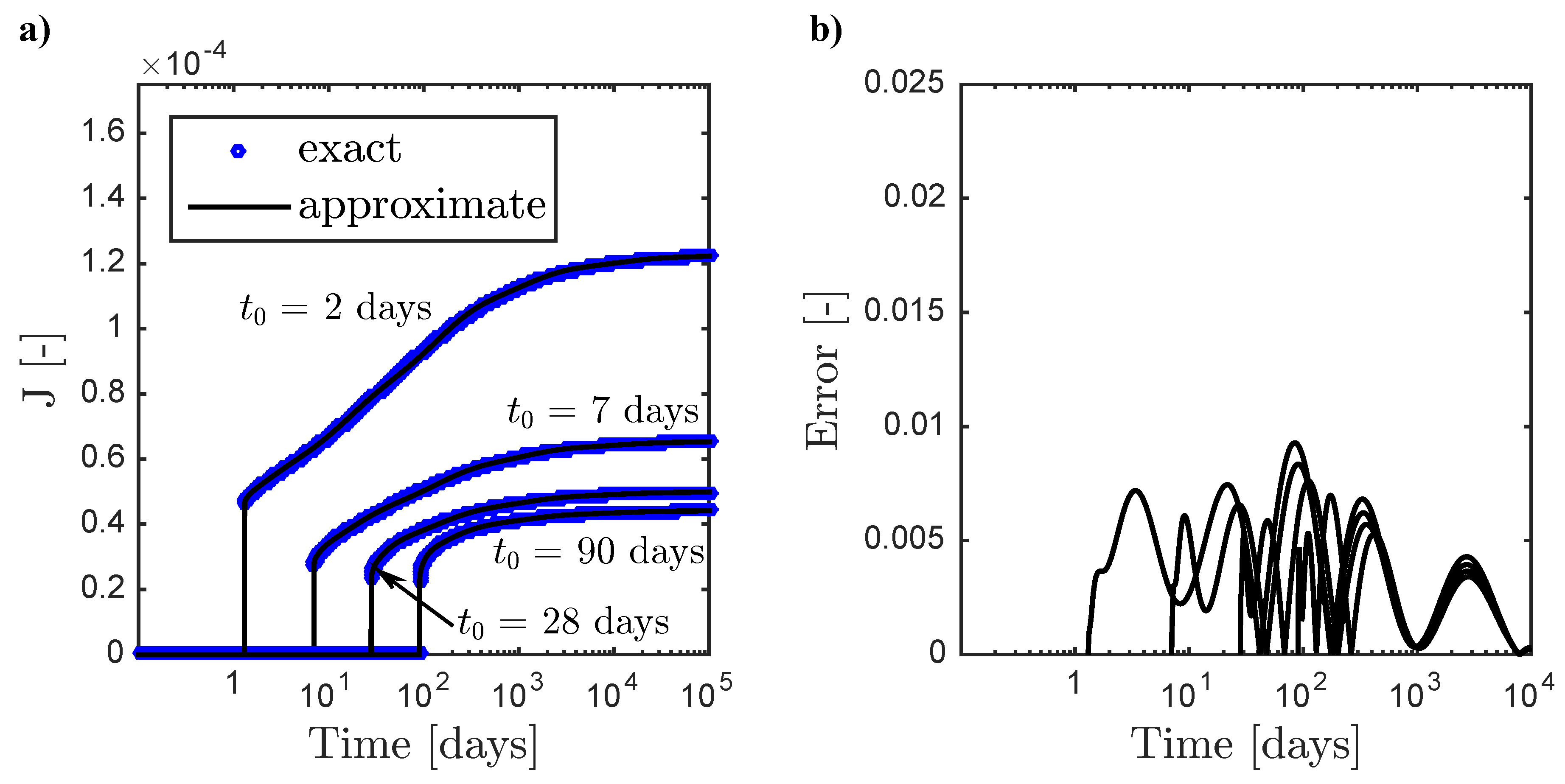
Figure 3.
Approximation of the B3 model compliance functions for different (2, 7, 28, and 90 days): Basic creep function (a) and absolute value of the approximating error (b); drying creep function (c) and absolute value of the approximating error (d).
Figure 3.
Approximation of the B3 model compliance functions for different (2, 7, 28, and 90 days): Basic creep function (a) and absolute value of the approximating error (b); drying creep function (c) and absolute value of the approximating error (d).
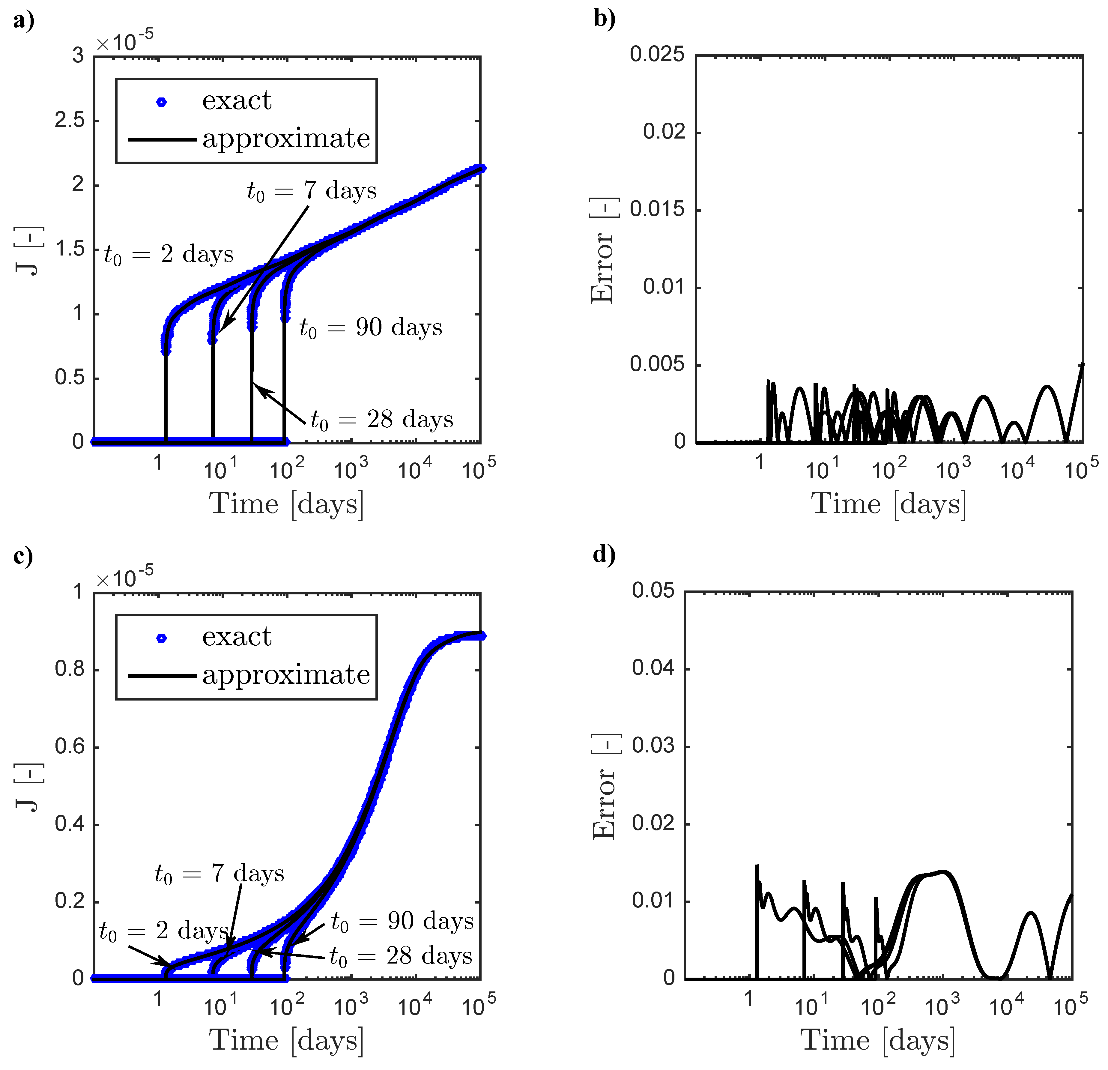
Figure 4.
Simply supported prestressed concrete beam: (a) Cross-section geometry in millimeters; (b) boundary conditions and loading; (c) load history; (d,e) finite element mesh.
Figure 4.
Simply supported prestressed concrete beam: (a) Cross-section geometry in millimeters; (b) boundary conditions and loading; (c) load history; (d,e) finite element mesh.

Figure 5.
Mid-span deflection of the beam in Figure 5 in logarithmic scale for different loading conditions obtained by 3D finite element analysis (with the amplified deformation) and by the beam theory with the effective modulus method.
Figure 5.
Mid-span deflection of the beam in Figure 5 in logarithmic scale for different loading conditions obtained by 3D finite element analysis (with the amplified deformation) and by the beam theory with the effective modulus method.
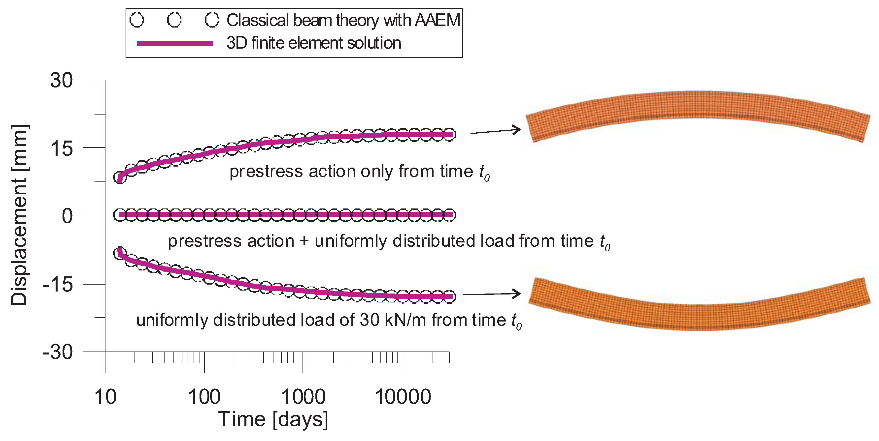
Figure 6.
(a) Evolution of the force in the prestress steel tendon for different loading conditions; (b–d) evolution of the normal stresses in the middle-span cross-section for the prestress action only, external distributed load only, and their combination, respectively.
Figure 6.
(a) Evolution of the force in the prestress steel tendon for different loading conditions; (b–d) evolution of the normal stresses in the middle-span cross-section for the prestress action only, external distributed load only, and their combination, respectively.
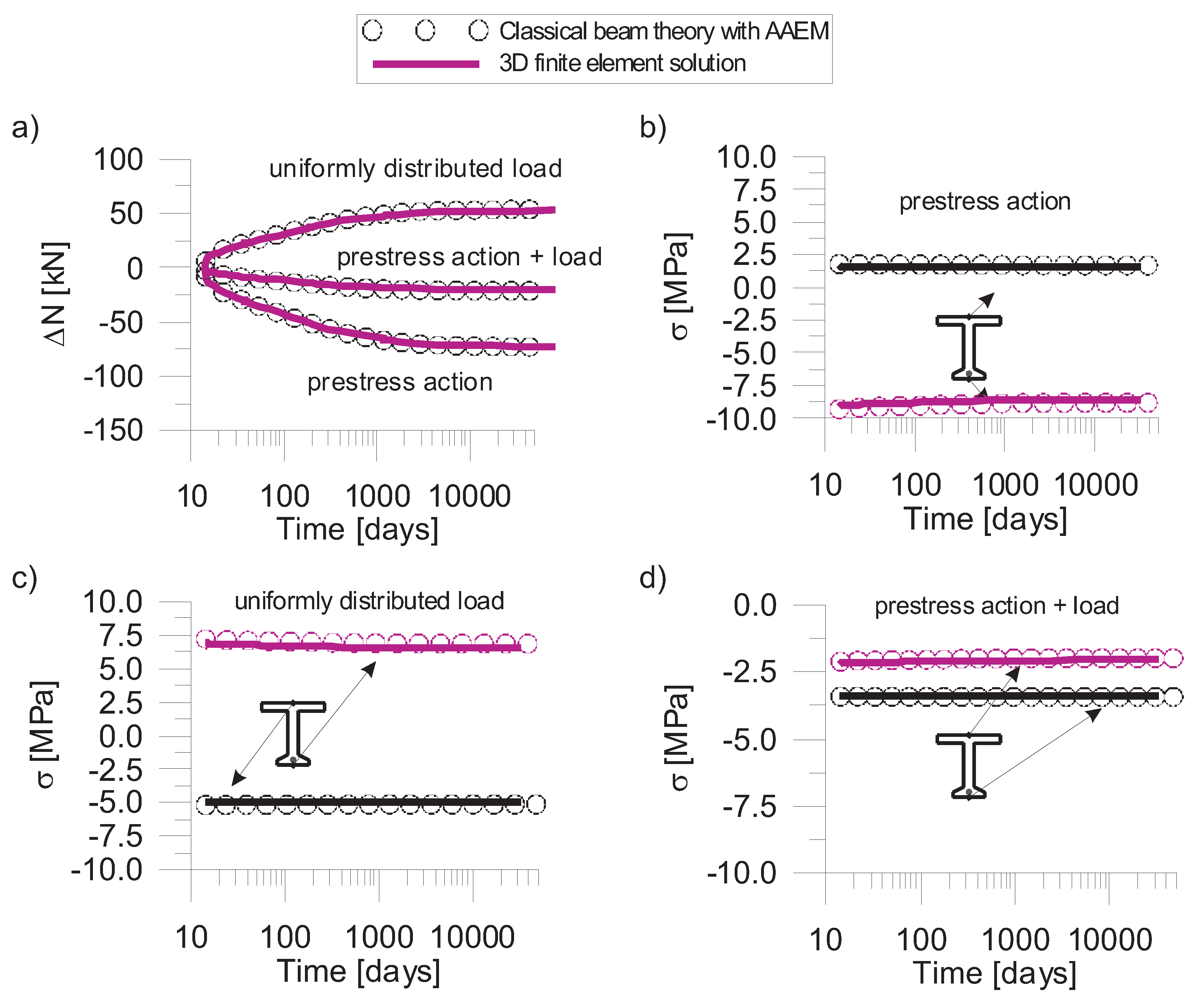
Figure 7.
Simply supported prestress beam under different load histories (a,c,e), on the left, and, on the right the corresponding deflections (b,d,f).
Figure 7.
Simply supported prestress beam under different load histories (a,c,e), on the left, and, on the right the corresponding deflections (b,d,f).
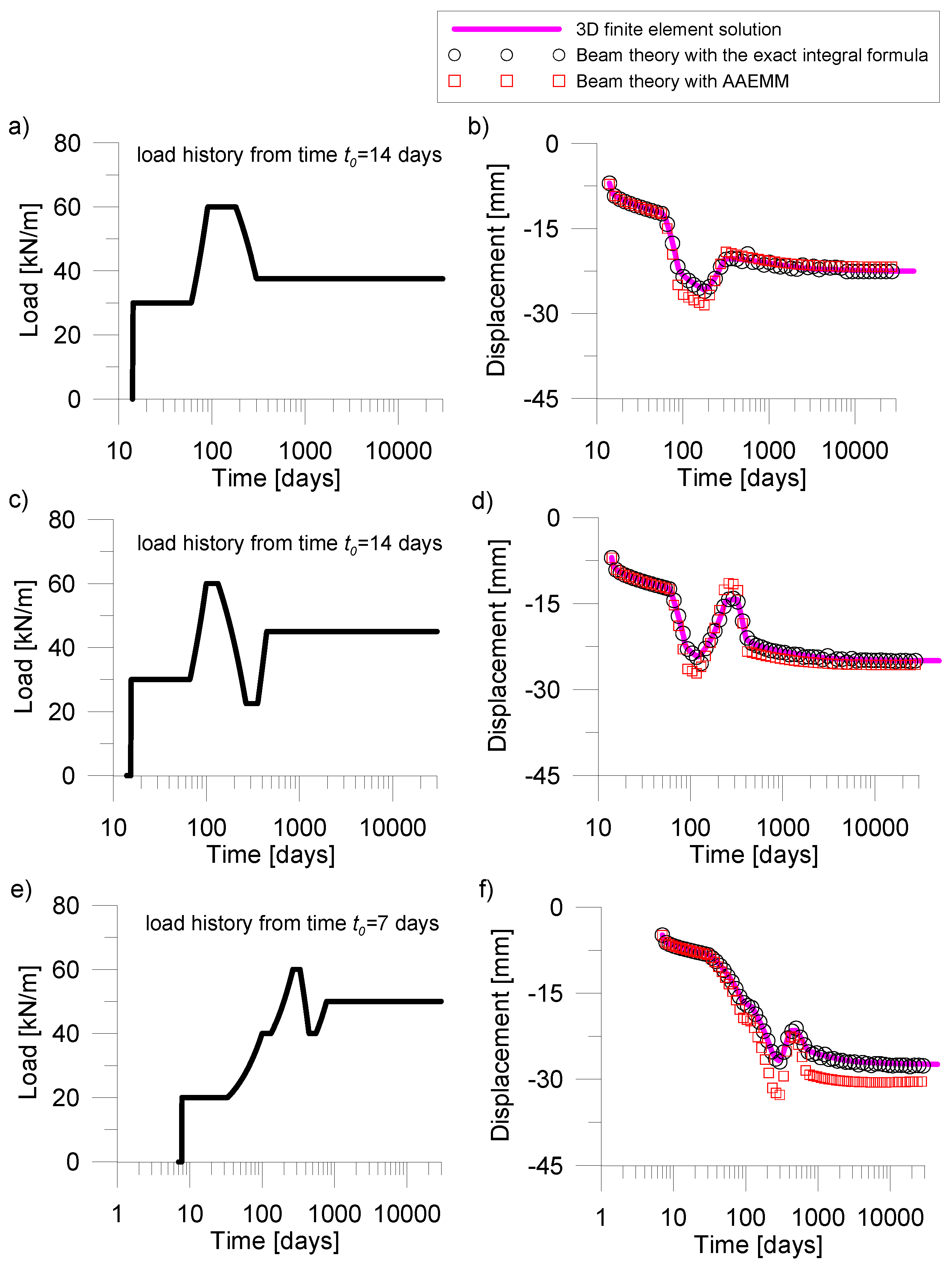
Figure 8.
Cantilever prestressed concrete box girder with variable cross-section: (a) Cross-section geometry at the fixed end; (b) cross-section geometry at the free end; (c) boundary conditions and loading history; (d,e) finite element mesh. All the lengths are in millimeters.
Figure 8.
Cantilever prestressed concrete box girder with variable cross-section: (a) Cross-section geometry at the fixed end; (b) cross-section geometry at the free end; (c) boundary conditions and loading history; (d,e) finite element mesh. All the lengths are in millimeters.
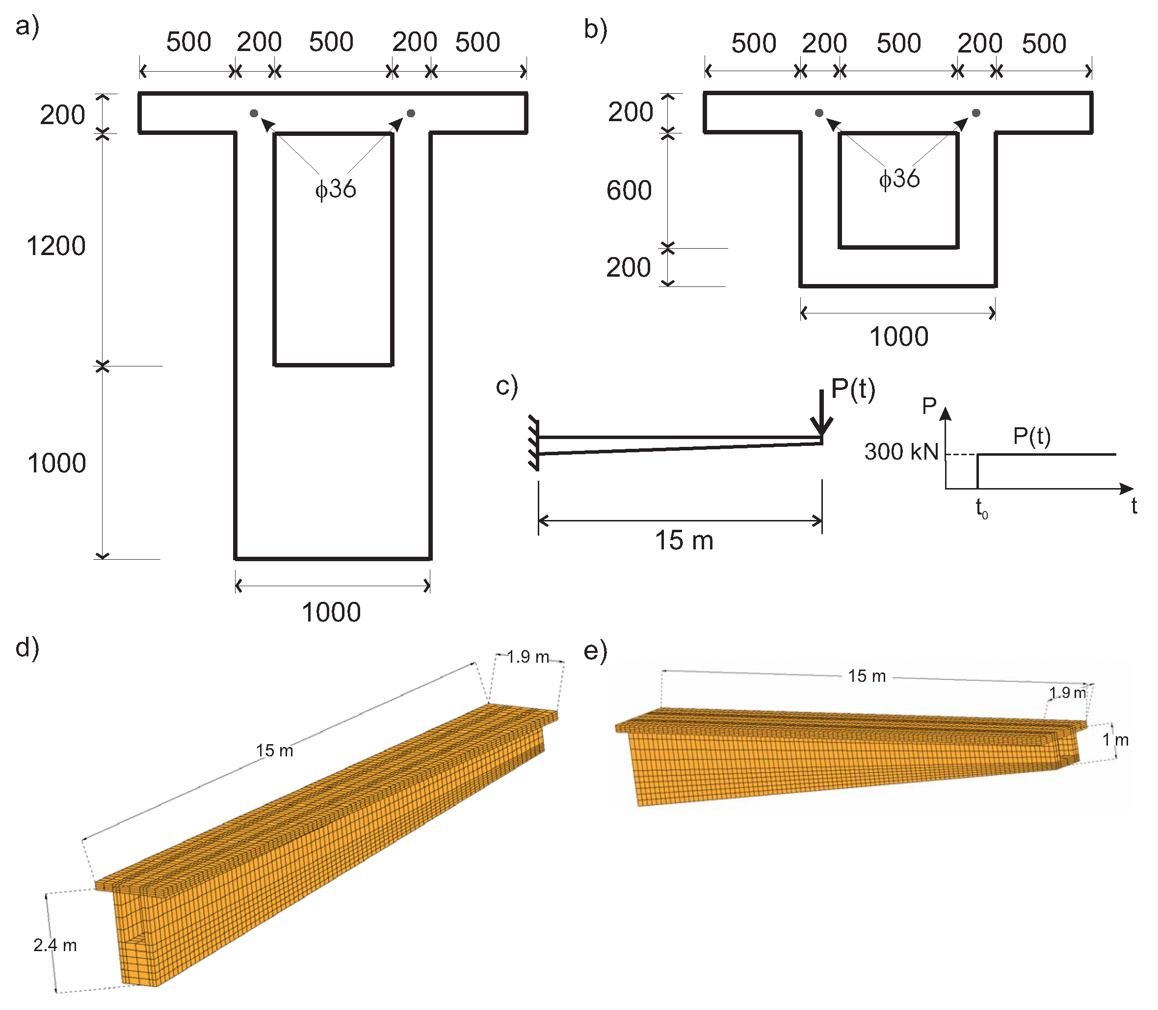
Figure 9.
Mid-span deflection of the beam in Figure 4 in logarithmic scale for different loading conditions obtained by 3D finite element analysis (with the amplified deformation) and by the beam theory with the effective modulus method.
Figure 9.
Mid-span deflection of the beam in Figure 4 in logarithmic scale for different loading conditions obtained by 3D finite element analysis (with the amplified deformation) and by the beam theory with the effective modulus method.
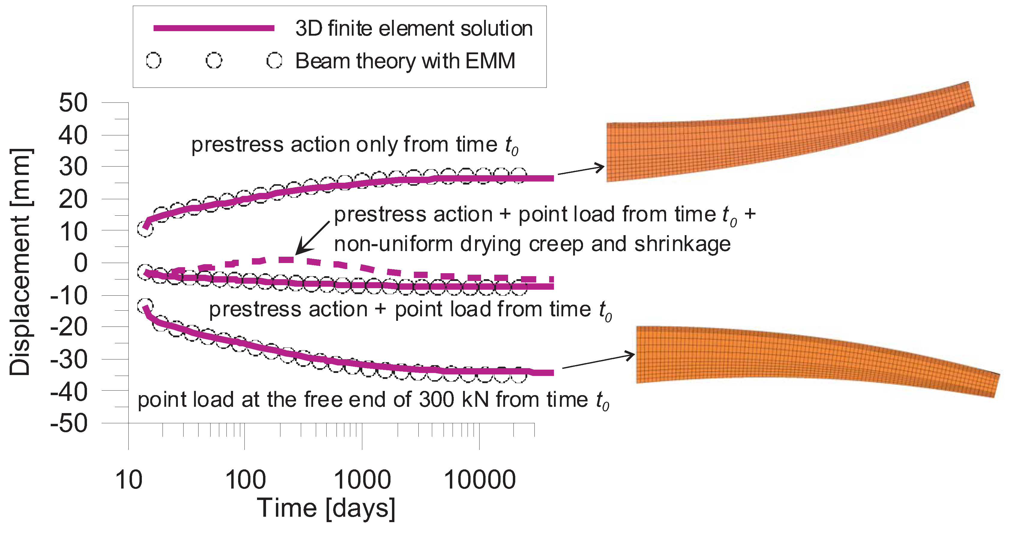
Figure 10.
(a) Evolution of the force in the prestress steel tendon for different loading conditions; (b–d) evolution of the normal stresses in the middle-span cross-section for the prestress action only, the point load only, and the both of them, respectively.
Figure 10.
(a) Evolution of the force in the prestress steel tendon for different loading conditions; (b–d) evolution of the normal stresses in the middle-span cross-section for the prestress action only, the point load only, and the both of them, respectively.
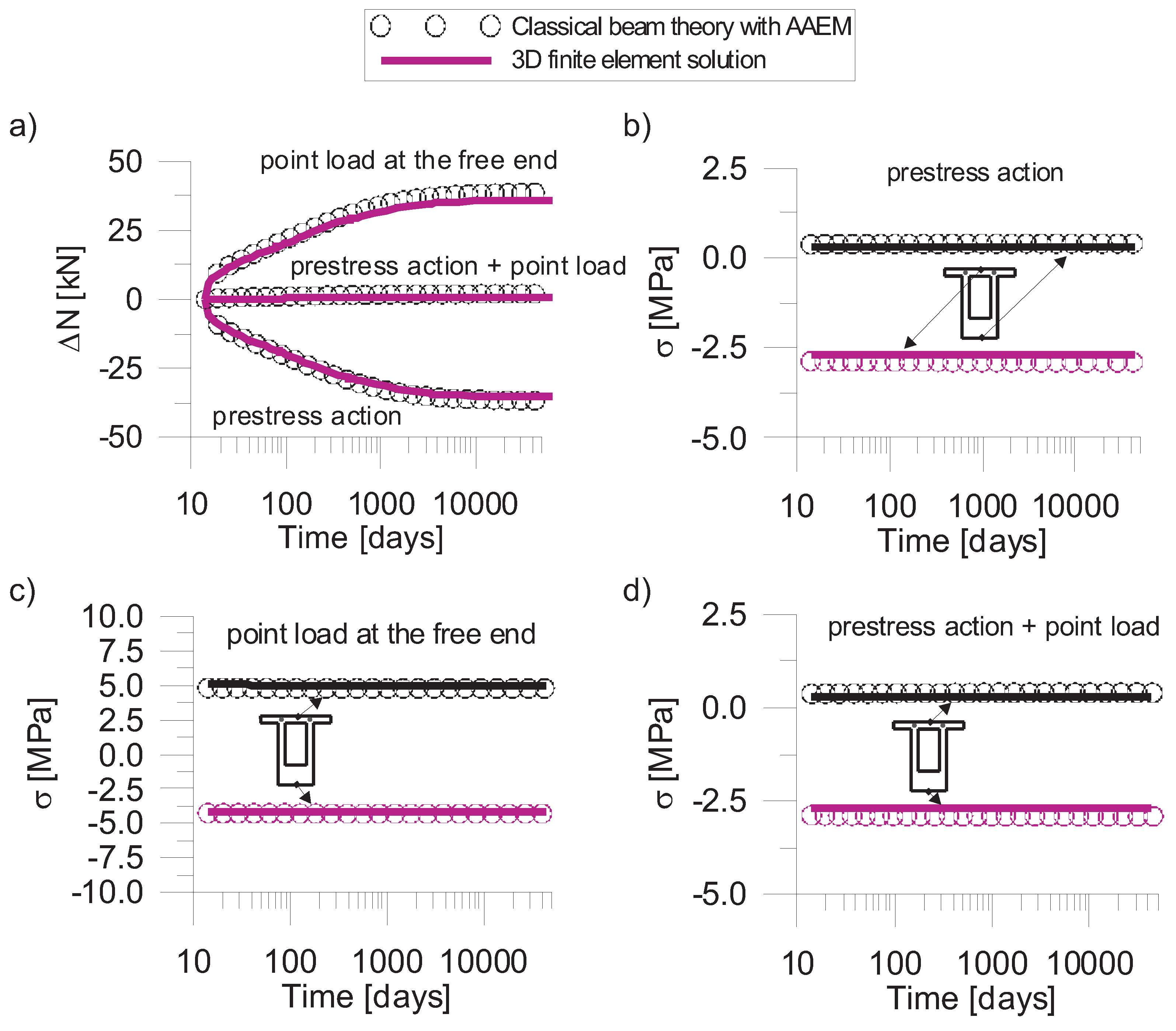
Figure 11.
Picture of the bridge during its construction.

Figure 12.
Project description: Upper view and longitudinal sections.
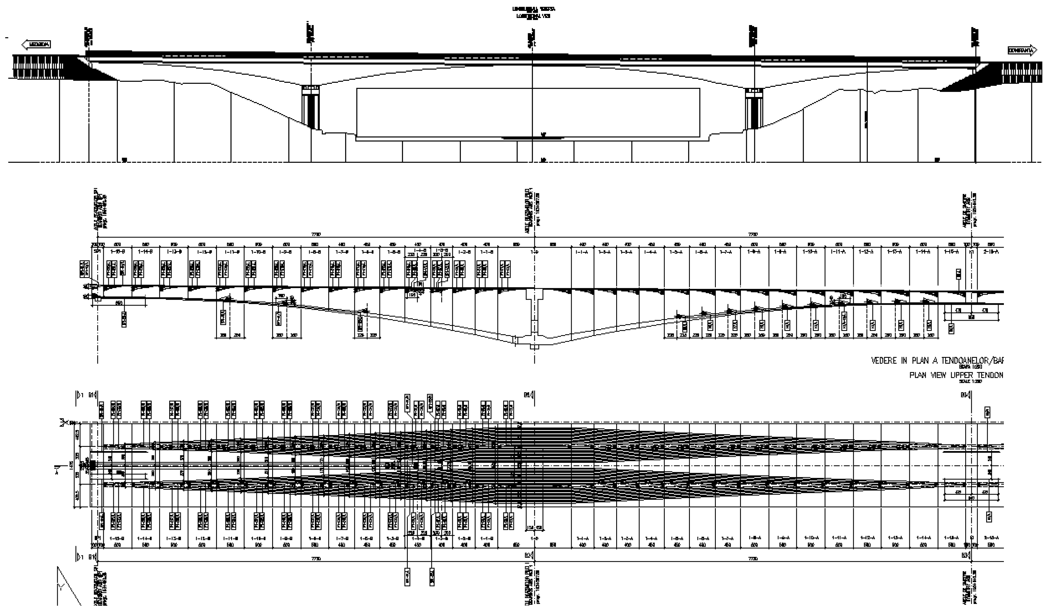
Figure 13.
Three-dimensional finite element mesh model of the bridge, the mesh of its different segments, and the mesh of the steel cables.
Figure 13.
Three-dimensional finite element mesh model of the bridge, the mesh of its different segments, and the mesh of the steel cables.
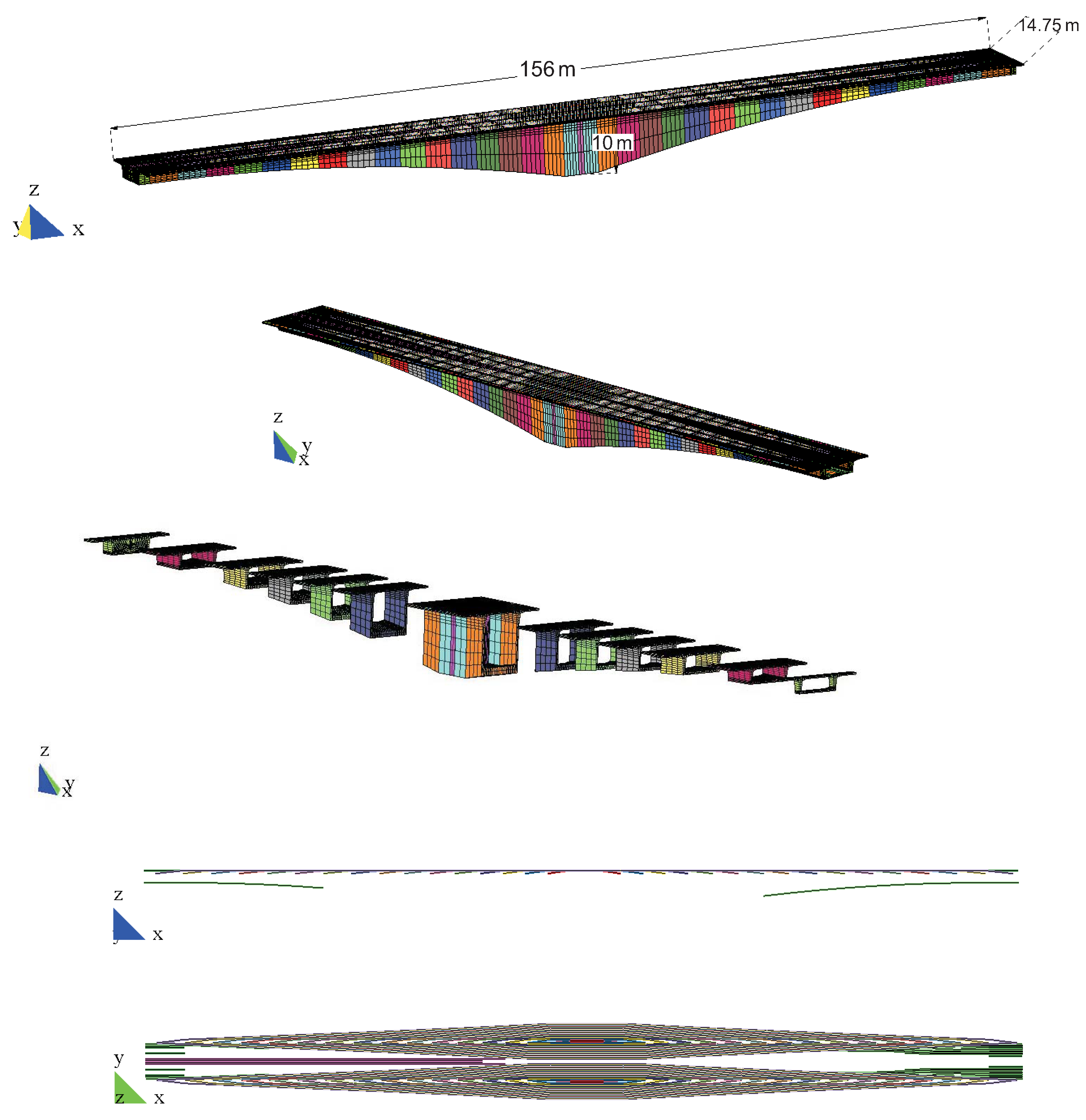
Figure 14.
Bridge deflection (positive if upward) in normal (a) and logarithmic (b) scale computed with different creep models.
Figure 14.
Bridge deflection (positive if upward) in normal (a) and logarithmic (b) scale computed with different creep models.

Figure 15.
Prestress loss in tendons at main (central) pier by EuroCode2 (a), ACI (b), and model B3 (c) in logarithmic scales.
Figure 15.
Prestress loss in tendons at main (central) pier by EuroCode2 (a), ACI (b), and model B3 (c) in logarithmic scales.
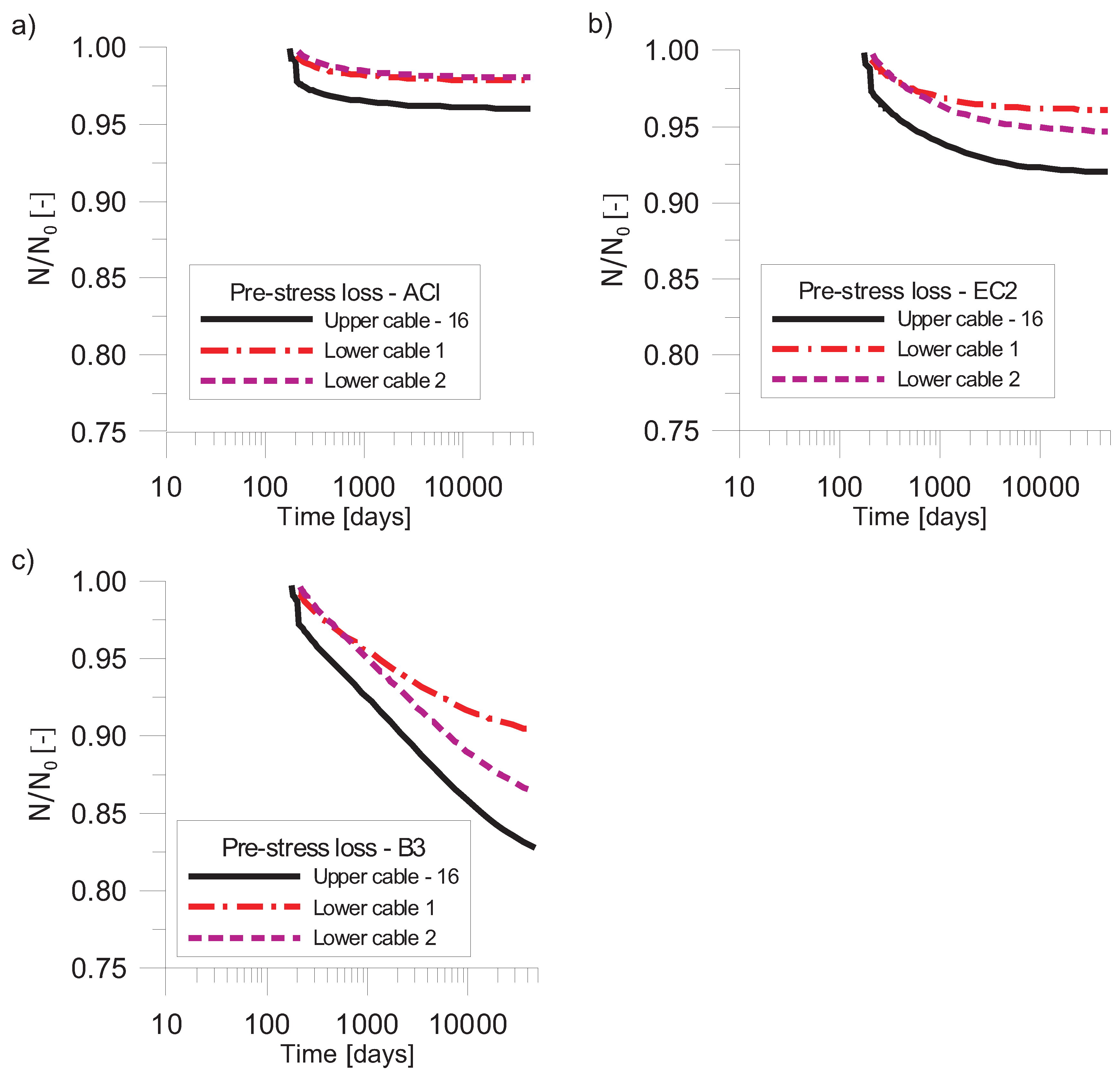
Figure 16.
Normal stresses in cross sections between different segments, computed with different creep model: EuroCode2 (a), ACI (b), and model B3 (c).
Figure 16.
Normal stresses in cross sections between different segments, computed with different creep model: EuroCode2 (a), ACI (b), and model B3 (c).


Table 1.
Level corrections of segments used in the bridge construction (positive sign means an upward correction).
Table 1.
Level corrections of segments used in the bridge construction (positive sign means an upward correction).
| Segment | Central Span [mm] | Side Span [mm] |
|---|---|---|
| 2 | 10.5 | 6.7 |
| 3 | 4.4 | 7.1 |
| 4 | 14.1 | 7.3 |
| 5 | 24.3 | 8.1 |
| 6 | 24.2 | 8.2 |
| 7 | 23.9 | 8.3 |
| 8 | 3.9 | 8.4 |
| 9 | 23.6 | 8.6 |
| 10 | 13.1 | 17.5 |
| 11 | 11.7 | 15.8 |
| 12 | 9.2 | 2.6 |
| 13 | 5.4 | −2.7 |
| 14 | −1.4 | −11.7 |
| 15 | −2.6 | 4.0 |
| 16 | 10.6 | 10.3 |
Table 2.
Details of the post-tension tendons and bars.
| Name | Position | Tendons | |||
|---|---|---|---|---|---|
| Strand Type | Number of Strands | Area [mm] | N [kN] | ||
| Cable 1 to 16 | Upper Pier | 0.6 normal | 12 | 1668 | 2335 |
| Lower cable | Lower side and central span | 0.6 compact | 22 | 3630 | 5082 |
| Upper cable | Upper side span | 0.6 normal | 12 | 1668 | 2335 |
| Bars | |||||
| [mm] | Area [mm] | N [kN] | |||
| thread-bars | Key segment | 36 | 1017 | 722 | |
| thread-bars | Abutment segments | 36 | 1017 | 722 | |
Table 3.
Effective thickness, , of the different elements in the cross sections.
| Segment | Upper Slab [mm] | Lateral Slab [mm] | Lower Slab [mm] |
|---|---|---|---|
| Diaphragm | 2304.70 | 4502.73 | 2200.00 |
| 1 | 517.82 | 865.58 | 1237.01 |
| 2 | 306.77 | 880.87 | 1143.65 |
| 3 | 306.82 | 885,71 | 1042.86 |
| 4 | 306.85 | 891,24 | 948.36 |
| 5 | 304.73 | 897.59 | 860.17 |
| 6 | 305.42 | 907.09 | 768.49 |
| 7 | 303.34 | 720.68 | 675.22 |
| 8 | 303.34 | 727.78 | 599.76 |
| 9 | 303.34 | 758.49 | 532.44 |
| 10 | 303.33 | 784.54 | 467.16 |
| 11 | 303.34 | 814.14 | 411.95 |
| 12 | 303.34 | 846.21 | 366.76 |
| 13 | 303.33 | 878.55 | 331.61 |
| 14 | 303.33 | 927.53 | 306.51 |
| 15 | 303.34 | 934.43 | 291.44 |
| 16 | 303.34 | 956.69 | 286.42 |
| B1 | 619.38 | 6869.47 | 700.00 |
| B3 | 303.33 | 926.99 | 286.42 |
Table 4.
Geometric characteristics of the bridge cross section and effective thickness, .
| Section | Area [m] | Segment Length [m] | Volume [m] | D [mm] |
|---|---|---|---|---|
| Diaphragm | 70.667 | 0.5 | 35.333 | 2437.007 |
| 1 | 23.111 | 3.5 | 80.891 | 603.483 |
| 2 | 19.117 | 4 | 76.468 | 514.435 |
| 3 | 17.812 | 4 | 71.252 | 499.910 |
| 4 | 16.590 | 4 | 66.363 | 485.120 |
| 5 | 15.446 | 4.5 | 69.511 | 470.055 |
| 6 | 14.259 | 4.5 | 64.169 | 453.102 |
| 7 | 12.258 | 4.5 | 55.162 | 403.015 |
| 8 | 11.410 | 4.5 | 51.349 | 389.807 |
| 9 | 10.654 | 5 | 53.274 | 377.120 |
| 10 | 9.922 | 5 | 49.610 | 363.916 |
| 11 | 9.302 | 5 | 46.508 | 352.999 |
| 12 | 8.794 | 5 | 43.972 | 341.620 |
| 13 | 8.482 | 5 | 42.410 | 336.480 |
| 14 | 8.136 | 5 | 40.682 | 327.697 |
| 15 | 7.949 | 5 | 39.743 | 323.048 |
| 16 | 7.880 | 5 | 39.402 | 321.317 |
| B1 | 9.417 | 2 | 36.352 | 370.549 |
| B3 | 8.317 | 1 | 8.3175 | 334.471 |
© 2020 by the authors. Licensee MDPI, Basel, Switzerland. This article is an open access article distributed under the terms and conditions of the Creative Commons Attribution (CC BY) license (http://creativecommons.org/licenses/by/4.0/).
Share and Cite
MDPI and ACS Style
Di Luzio, G.; Cedolin, L.; Beltrami, C. Tridimensional Long-Term Finite Element Analysis of Reinforced Concrete Structures with Rate-Type Creep Approach. Appl. Sci. 2020, 10, 4772. https://doi.org/10.3390/app10144772
AMA Style
Di Luzio G, Cedolin L, Beltrami C. Tridimensional Long-Term Finite Element Analysis of Reinforced Concrete Structures with Rate-Type Creep Approach. Applied Sciences. 2020; 10(14):4772. https://doi.org/10.3390/app10144772
Chicago/Turabian StyleDi Luzio, Giovanni, Luigi Cedolin, and Carlo Beltrami. 2020. "Tridimensional Long-Term Finite Element Analysis of Reinforced Concrete Structures with Rate-Type Creep Approach" Applied Sciences 10, no. 14: 4772. https://doi.org/10.3390/app10144772
Note that from the first issue of 2016, this journal uses article numbers instead of page numbers. See further details here.