Nondestructive Evaluation of Solids Based on Deformation Wave Theory


1
Department of Chemistry and Physics, Southeastern Louisiana University, Hammond, LA 70402, USA
2
Department of Mechanical Engineering, Niigata University, Niigata 9502181, Japan
*
Author to whom correspondence should be addressed.
Appl. Sci. 2020, 10(16), 5524; https://doi.org/10.3390/app10165524
Submission received: 19 May 2020
/
Revised: 16 July 2020
/
Accepted: 1 August 2020
/
Published: 10 August 2020
(This article belongs to the Special Issue Nondestructive Testing (NDT): Volume II)
Abstract
:The application of a recent field theory of deformation and fracture to nondestructive testing (NDT) is discussed. Based on the principle known as the symmetry of physical laws, the present field theory formulates all stages of deformation including the fracturing stage on the same theoretical basis. The formalism derives wave equations that govern the spatiotemporal characteristics of the differential displacement field of solids under deformation. The evolution from the elastic to the plastic stage of deformation is characterized by a transition from longitudinal (compression) wave to decaying longitudinal/transverse wave characteristics. The evolution from the plastic to the fracturing stage is characterized by transition from continuous wave to solitary wave characteristics. Further, the evolution from the pre-fracturing to the final fracturing stage is characterized by transition from the traveling solitary wave to stationary solitary wave characteristics. In accordance with these transitions, the criterion for deformation stage is defined as specific spatiotemporal characteristics of the differential displacement field. The optical interferometric technique, known as Electronic Speckle-Pattern Interferometry (ESPI), is discussed as an experimental tool to visualize those wave characteristics and the associated deformation-stage criteria. The wave equations are numerically solved for the elastoplastic stages, and the resultant spatiotemporal behavior of the differential displacement field is compared with the experimental results obtained by ESPI. Agreement between the experimental and numerical results validates the present methodology at least for the elastoplastic stages. The solitary wave characteristics in the fracturing stages is discussed based on the experimental results and dislocation theory.
1. Introduction
Structures collapse unexpectedly. Continuous application of external loads, even if their strength is considerably lower than the ultimate strength of the material, causes fractures. The current load level observed or associated deformation data is not reliable information to predict fracture. It is known that fracture is led by a defect and that defects grow in the scale level from the atomistic to macroscopic. Dislocations [1] are typical atomistic defects and their propagation is responsible for the deformation to evolve from the elastic to plastic regime. It is known that in the plastic regime the dislocations react to the stress field and lead to the generation of macroscopic defects. Egorushkin [2] formulates the dynamics of dislocation as a wave phenomenon. However, it is difficult to connect dislocation behaviors and macroscopically observable phenomena. In other words, on the one hand we know that the propagation of dislocation initiates plastic deformation. On the other hand, we cannot identify the initiation of plastic deformation as a macroscopically observable quantity, except as the yield point on the stress–strain curve. From the nondestructive testing (NDT) perspective, it is unrealistic to measure the stress-stain characteristics of test objects in the field. It is desirable to develop a methodology that allows us to diagnose the initiation of plastic deformation and the subsequent evolution of the deformation toward the final fracture.
One immediate problem in such methodological development is that prevailing deformation theories are phenomenological and, thereby, stage specific. Elastic theories [3,4,5] describe the stress strain relationship in the elastic regime. Most plastic deformation theories [6,7] describe plastic behavior by either mathematically modeling the constitutive relation in the plastic regime or formulating the plasticity based on the energy dissipation. Fracture [8] is treated as an independent phenomenon of deformation. This situation makes it difficult to describe the transition from one deformation regime to another.
In this work, we propose that the application of a recent field theory [9] of deformation and fracture can be a solution to the problem. Being based on the physical principle known as the local symmetry of theory [10,11,12] (See Appendix A), this theory has a mechanism to describe deformation and fracture on the same theoretical basis. It formulates all stages of deformation and fracture based on the wave equation derived from the equation of motion that governs the dynamics of a unit volume in a deforming object. Different stages of deformation are characterized by different forms of resistive force that the unit volume exerts in response to the external load. This difference in the resistive force alters some terms of the wave equation yielding different wave solutions. Details about the wave equation and wave solutions will be discussed later in this paper. In short, the elastic stage is represented by non-decaying longitudinal waves, the early stage of plastic deformation is by decaying longitudinal and transverse waves, the developed plastic stage (the pre-fracture stage) is by travelling solitary waves, and the fracturing stage is by standing solitary waves. In all stages, these waves carry the stress energy that is caused by the external load.
These forms of deformation waves in association with the corresponding deformation stages have been observed by several authors. In a tensile experiment of an aluminum alloy specimen, we [13] observed that a transverse displacement wave started to appear near the yield point and decayed towards the final fracture of the specimen. In refs. [14,15,16], the authors identified a solitary-wave like pattern in the displacement field of tensile loaded metal plate specimens and observed that the pattern becomes stationary when the specimen broke. Ref. [17] reports simlar observation of a solitary-wave like pattern in the displacement field for a cyclic loaded metal specimen. Ref. [18] explains these experimentally observed behaviors of the solitary-wave like patterns based on a Korteweg-de Vries (KdV)-type [19] solitary wave solution. The formation of solitary waves from non-solitary waves has also been reported. Ziv and Shmuel [20] discuss the coalescence of longitudinal and shear waves to form shock waves in soft materials. Lints [21] et al. discuss the formation of solitary waves in a carbon fiber reinforced polymer with non-solitary ultrasonic excitation.
The use of the above-mentioned, stage-specific behavior of deformation waves makes the present NDT unique. Various waves are widely used in conventional NDT methods. In these methods, a linear wave is typically applied to the test object as the input and the reflected or transmitted (the output) wave is monitored. The structural or mechanical properties of the object are diagnosed through analysis of the output wave based on a certain property of the wave. Acoustic imaging [22,23] identifies abnormality from the difference in the acoustic impedance, which alters the reflection coefficient for the input wave; hence, making a contrast in the output wave. Scanning Acoustic Microscopy [24,25] uses the interference between the input and reflected ultrasound waves to characterize the property of the subsurface region of a specimen. X-ray diffractometry [26,27] uses diffraction to find the lattice constant of the object material. In relatively new methods, solitary waves are also used as the input wave [28,29,30]. As a nonlinear wave, a solitary wave changes its wave form depending on the material’s property. This feature makes it possible to detect abnormality that linear input waves are unable to detect.
The present NDT algorithm is intrinsically different from these methods in the following sense. Instead of analyzing the output signal that results from a certain input wave, it analyzes the materials’ self-generated deformation waves. In other words, while conventional techniques analyze the material’s response to the input wave, the present method characterizes the material’s response to the applied load as a wave phenomenon. Thus, the observed wave exhibits the dynamics that governs the deformation behavior for the respective stages. By knowing the dynamics for each stage and the associated features of the deformation wave, we can diagnose the current status of deformation and its future trend.
Based on the stage-specific specific behaviors of the deformation wave, we have derived field theoretical criteria of deformation stages [31]. The criteria describe the spatiotemporal behavior of the displacement field in the elastic, plastic, pre-fracture, and fracture stages. In accordance with the above-mentioned form of the displacement wave, the displacement field expressed in the principal coordinates is rotation-free (because the wave is longitudinal) in the elastic stage, rotational (because the wave has transverse component due to the shear strain) in the plastic stage, localized in a small region (because the wave is a solitary wave), but dynamic in the pre-fracture stage, and localized in a small region and static (because the solitary wave becomes standing) in the fracture stage (more detailed descriptions of the characteristics of the displacement field will be discussed later in this paper).
In refs. [31,32], we demonstrated the deformation stage criteria based on these qualitative features of the displacement field. Using the optical interferometric technique known as Electronic Speckle-Pattern Interferometry (ESPI) [33,34,35], we continuously visualized the displacement field of metal plate specimens as the test machine applied a tensile load. With a pre-defined time interval small enough to resolve the stress-strain curve, the ESPI setup displayed the displacement field as full-field, two-dimensional optical interferometric image data. This arrangement is convenient for the diagnosis against the deformation stage criteria because the interferometric fringes, which represent contours of differential displacement components, readily exhibit the qualitative features of the displacement field (rotation-free etc). The diagnosed deformation stages were found to be consistent with the stress–strain characteristic obtained during the same tensile experiment.
In this study, the idea of using the ESPI fringe patterns is extended in order to visualize the wave characteristics of the displacement field. We analyzed the fringe pattern for several consecutive time steps in several deformation stages, and compared the spatiotemporal behavior of the displacement field against numerically generated deformation wave forms. Here, the numerical wave forms were obtained by solving the above-mentioned wave equation without assuming a constitutive model (except for the use of Poisson’s effect). It has been found that the visualized displacement field shows the same spatiotemporal behavior as the numerical wave forms. This allowed us to confirm the validity of the proposed wave-dynamics based diagnosis of deformation status via direct comparison with the wave forms. The aim of this paper is to report our observations in this investigation. The present paper is organized in the following way. Section 2 presents the gist of the field theory, including the deformation stage criteria and the explicit form of the wave equation for all the stages. Section 3 describes the experimental and numerical methods that were used in this study. Section 4 presents the experimental and numerical results and discusses the observations based on the wave dynamics. The semi-quantitative agreement between the experimentally observed displacement field and the numerical result obtained as solutions to the wave equation encourages further investigation of the subject toward the development of more quantitative NDT algorithm based on the present field theory.
2. Field Theory of Deformation and Fracture
2.1. Field Theory Overview
The present field theoretical approach has been derived from the concept of physical mesomechanics. Panin et al. [36] are the first to introduce the concept of mesoscopic scale-level to deformation dynamics and developed physical mesomechanics. In his paradigm of deformation, Panin characterizes plastic deformation as shear instability associated with the finite volume defined as the deformation structural element (DSE). When a deformation enters the plastic regime, the solid gains rotational degrees of freedom in the deformation dynamics and the DSE is the unit volume of material rotations. Applying the concept of the (gauge) field theory [11], he formulates dynamics of plastic deformation as the spatiotemporal behavior of the compensation (gauge) field that accommodates the rotational degree of freedom in the linear (non-rotational) elastic theory.
The present field theory is an extension of Panin’s paradigm to all stages of deformation and fracture. The wave characteristics of the deformation field for each stage of deformation can be summarized, as follows. In the elastic regime, the solid responds to the external force with elastic oscillatory motion that is transferred as a longitudinal wave known as the elastic compression wave. This dynamics is described by Young’s modulus and Poisson’s ratio. In the principal coordinate system, this leads to zero shear components in the distortion tensor. In the plastic regime two things happen. First, the material loses the shear stability, and consequently, the shear components become active in the distortion tensor. In the wave dynamics, this generates a transverse wave. Second, the material exhibits energy damping that is associated with the nonlinear behavior of the velocity filed. This makes the deformation irreversible, causing the longitudinal and transverse waves to decay. In the late stage of plastic deformation (the pre-fracture stage), the material’s elasticity becomes nonuniform. This induces dispersion (as the elasticity is not represented by a single constant), as is the case of the classical dispersion observed in a string on an elastic medium [37] or in a granular chain [38]. When the nonlinear term associated with the above-mentioned energy damping mechanism and the dispersion term of the wave equation satisfy a certain condition, the decaying wave takes the form of a solitary wave that travels carrying the stress energy. Fracture is characterized as the final stage of deformation where the material loses the mechanism to dissipate the stress energy in the form of traveling wave. Consequently, the mechanical wave, at this stage it is a solitary wave, becomes standing and unable to carry the stress energy. As a result, the stress becomes motionless at a certain location of the material. It follows that the generation of discontinuity becomes the only mechanism for the material to balance the energy.
Figure 1 illustrates the gist of the present field theory. The theory postulates that a solid at any stage of deformation possess local elasticity. The dynamics of local elasticity is represented by the deformation gradient tensor that describes Hooke’s law [39]. Here, and represent the coordinates of a reference point, expressed with the local coordinate system, after and before the deformation occurs, respectively. Hooke’s law is orientation preserving [4], because the applied force and the resultant stretch or compression are parallel to each other. In other words, it describes translational dynamics. Continuum mechanics extends Hooke’s law by expressing the compression (stretch) in orthogonal directions to the applied tensile (compressive) force with a Poisson’s ratio. The deformation in the orthogonal directions are parallel to the corresponding orthogonal axis, and hence the dynamics is still translational. The three elliptical shapes in Figure 1 represent three segments inside the same solid object that undergo elastic deformation in their own orientation. Being a tensor describing an orientation preserving phenomenon, the deformation gradient tensor for one segment cannot describe other segments unless they are oriented in the same direction. Figure 1 illustrates the situation, where the three elastic segments are not oriented in the same direction. This means that, in this situation, the elasticity of the three segments cannot be described by a common (global) coordinate system.
Consider how we can describe the elasticity of all the segments commonly with a global coordinate system. A solution is that we align all of the segments to the same orientation by introducing an additional field. This type of field is referred to as a connection (gauge) field [11], as they logically “connect” local dynamics. We can incorporate the dynamics that are associated with the connection field by considering the effect as a potential [11]. In Figure 1, “Potential A” represents this potential. In other words, we incorporate the dynamics associated with difference in the actual orientation among the segments into the effect of the potential and interpret that the three segments are experiencing elastic deformation at the global level. In this fashion, we can formulate the nonlinearity in the plastic regime by finding the dynamics that the connection field obeys. Note that the irreversibility of plastic deformation is not formulated by the connection field. Instead, it is represented by the energy dissipative part of the dynamics of the connection field. By applying the Lagrangian formalism to the dynamics of the connection field, a set of field equations that are discussed in the next section are derived.
2.2. Field Equations
The detailed procedure to derive the field equations is described elsewhere [9,40,41]. In short, it can be described as follows. The first step is to find the Lagrangian associated with the potential . As clear from its role to rotate the local segments so that they are all aligned in a common orientation and, therefore, the dynamics can be formulaically expressed by Hooke’s law, has a dimension of displacement. In general, Lagrangian takes the form of kinetic energy minus potential energy. In the present case, it is natural to interpret that the kinetic energy is associated with the temporal derivative (the velocity) of . On the other hand, the potential energy depends on the type of the dynamics, as will be discussed below for elasto-plastic dynamics and fracture dynamics. The second step is to derive the field equations by using the Lagrangian in the Euler-Lagrangian equation of motion for the given dynamics. The active terms in the Euler-Lagrangian equation of motion also depends on the type of the dynamics that the system experiences.
2.2.1. Elasto-Plastic Dynamics
A rigorous analysis that is based on the gauge theoretical approach identifies the Lagrangian density for the elasto-plastic dynamics, as follows.
Here, G is the shear modulus, is the phase velocity of the wave characteristics, and and are the temporal and spatial components of the charge of symmetry, respectively. and are related to , as follows.
Here, indexes represent the spatial coordinate variables.
The Euler–Lagrangian equation of motion in this case is given as follows.
where . Substitution of Equation (1) into Equation (4) yields the following field equations.
Multiplication of G on both-hand sides allows us to rewrite Equation (6) in the following form.
The left-hand side of Equation (7) is in the form of mass times acceleration. Thus, Equation (7) can be interpreted as an equation of motion. The first and second terms on the right-hand side of Equation (7) can be interpreted as the transverse (shear) force and longitudinal force acting on the unit volume that is represented by density (see Chapter 5 of ref. [9]). Analysis indicates that the longitudinal force takes the following forms in the pure elastic and pure plastic dynamics, respectively.
Here, is the Lamé’s first parameter, is a material constant (See Chapter 5 of ref. [9]), is the displacement vector. In Appendix B, conceptual images of the shear force that are represented by and the longitudinal fore represented by are illustrated. ( appearing on the right-hand side of Equation (8) is the displacement vector associated with elastic force law and on the right-hand side of Equation (9) is the temporal derivative of vector potential whose dimension is displacement. Strictly speaking, the physical meaning of displacement is different from . However, recent theoretical consideration indicates that, formulaically, we can replace with and interpret it as the total displacement vector (see Appendix C). Hereafter in this paper, is used to represent the displacement vector and ).
Equations (8) and (9) indicate that the form of the longitudinal force term differentiates plastic deformation from elastic deformation. When the deformation is elastic, the longitudinal force is proportional to the differential displacement , which is interpreted as the three-dimensional stretch or compression of a unit volume. When the deformation is plastic, the longitudinal force is proportional to the velocity through a variable coefficient . This relation can be interpreted as the proportionality is not connected by a constant but a variable coefficient. These two longitudinal forces are interpreted as material’s resistant force; with the elastic dynamics the unit volume resists the external force exerted by the neighboring unit volume via elastic force (8), and with the plastic dynamics the unit volume resists the external force via the velocity damping force (9). The former force induces traveling waves and the latter force causes the wave to decay. More will be discussed regarding the wave dynamics below.
2.2.2. Fracture Dynamics
The Lagrangian for the fracture dynamics is as follows.
As compared with Lagrangian density (1), expression (10) has the extra term at the end of the right-hand side. This term represents the potential energy that is associated with the secondary spatial derivatives of displacement. Because the first-order derivative of displacement is strain, this term represents the potential energy associated with the spatial gradient of the strain. In the pre-fracturing stage, deformation becomes so nonuniform that the differential strain generates potential energy. In other words, this term represents how nonuniform the deformation field becomes.
In this case, since the Lagrangian density has a term depending on the second-order spatial differential term, the Euler–Lagrangian equation of motion has the extra term.
Tensile experiments [14,15,16,17] indicate that under the pre-fracture condition, is one-dimensional and oriented at approximately 45 to the tensile axis. Under the one-dimensional condition, the substitution of Equation (10) into Equation (11) yields the following field equation corresponding to (7).
Here, is the axis set along the one-dimensional . Accordingly, and in the first and second terms on the right-hand side are the one-dimensional form of and appearing in Equations (8) and (9), respectively. It is reasonable to assume that a fracturing unit volume does not exert elastic resistant force proportional to the volume expansion. When the volume is about to fracture, the resistant force does not increase as the volume stretches. Instead, the surrounding unit volumes that border the fracturing unit volume at and exert elastic force proportional to the local stretch occurring within the small region expressed by (in other words, the strain energy is associated with the differential strain, not strain. See Figure 2 and the associated text). The third term on the right-hand side of Equation (12) represents this force. Thus, we can set the first term on the right-hand side of Equation (12) to null and rewrite the equation, as follows.
As will be discussed later in this paper this assumption is consistent with the experiment.
2.3. Conditions for Deformation Stages and Wave Equations
2.3.1. Linear Elastic Stage
When the deformation dynamics is linear elastic, Hooke’s law and Poisson’s effect are the only governing laws. Under this condition, the dynamics can be expressed in one coordinate system for the entire object. In terms of the concept that is depicted by Figure 1, there is no distinction between the global and local coordinate systems. In this situation, rotation represents rigid-body rotation, as defined by continuum mechanics. The entire entity (in the present context the block for which stress and strain are argued) undergoes a common rotation. Therefore, its spatial dependence is null. The force law is described by means of elastic force proportional to the local stretch or compression. Thus, we can express the linear elastic condition, as follows.
When the principal axis coordinate system is used to express the dynamics, the corresponding stress and strain tensors are diagonal. They have only normal components and all shear components become null. This is contrastive to the elasto-plastic dynamics, as discussed in the following section. In Appendix D, a short argument is made to show that the same physical elastic deformation raises shear components in the stress and strain tensors when a non-principal axis coordinate system is used.
2.3.2. Elasto-Plastic Stage
The term in field Equation (6) represents shear elastic force. When this force is active, the deformation becomes nonlinear at the global level. Accordingly, in principle, we can define a nonlinear elastic condition. However, tensile experiments [13] indicate that, when the deformation shows a nonlinear behavior represented by (the shear component becomes non-zero when expressed in the principal coordinate system), the stress–strain curve exhibits irreversible stretch. Thus, it is reasonable to combine the nonlinear elasticity and plasticity. Accordingly, we express the elasto-plastic condition, as follows.
The meaning of condition (16) is straightforwardly understood by recalling that Hooke’s law is orientation preserving, as mentioned earlier in this paper. When different blocks start to undergo linear elastic deformation in their own orientations, as schematically illustrated in Figure 1, it becomes impossible to describe the dynamics at the global level based on an orientation-preserving force law. This is when the vector potential plays its role as the orientation aligner. Referring to Figure 1, we can argue , as follows. Assume that the plane that is illustrated in Figure 1 is the plane of a Cartesian coordinate system. The rotation vector for each of the three blocks has only a z component. Under this situation, with the negative sign in front, the force term in equation of motion (7) can be interpreted as the elastic resistive force that the material exerts at the boundary of two neighboring unit volumes (see Figure A2a) to oppose the rotational deformation. This resistive force has in-plane components, as shown on the right-hand side of Equation (18), because the rotations that the force opposes are around an out-of-plane axis.
While condition (16) illustrates the non-linear elastic resistive behavior of plasticity, condition (17) illustrates the linear energy-dissipative behavior of plasticity. Being proportional to the particle velocity , it represents that the material exerts a velocity-damping, longitudinal force as an energy dissipative resistive force. Importantly, the damping coefficient is a variable depending on the divergence of the particle velocity vector field. The quantity can be interpreted as the rate of the local volume expansion. This variable nature of the damping coefficient has a significant meaning in the late stage of plastic deformation. The higher the volume expansion rate the greater the damping effect. This causes the self-driven nature of the evolution to fracture at this stage of deformation; the higher the volume expansion rate, the more energy dissipative the dynamics becomes. Hence, this makes the energy balance with the external load tend toward irreversible energy consumption as opposed to recoverable elastic energy. Note that this damping force can be interpreted as the energy dissipative resistive force that the material exerts making the resultant deformation irreversible.
2.3.3. Fracturing Stage
When a unit volume is fracturing, the elastic force terms become inactive. It is possible that the velocity damping force is still active in the one-dimensional form used in Equation (13). Thus, we can express the fracture condition, as follows.
The first fracture condition (19) indicates that when the fracture condition is satisfied the material does not exert elastic resistive force. The second fracture condition (20) indicates that the material exerts energy dissipative force in response to the external load. The second condition is further classified into recoverable fracture and final fracture conditions.
In conditions (21) and (22), ensures Newton’s third law. The energy dissipative force is the reaction to the external force. Condition (22) is interpreted as the final fracture condition because of the following argument. In condition (20), if the left-hand side is non-zero and on the right-hand side, it follows that . This condition means that the particles diverge at the infinite rate from the unit volume, which apparently indicates the generation of material discontinuity. It is interesting to note that material fracture resembles electric discharge of gasses [42]. More specifically, recoverable fracture resembles spark discharge [43] and final fracture resembles arc discharge. Spark discharge in gas media is similar to arc discharge, but it does not cause electrical breakdown of the gas [44]. These resemblances between fractures and electric discharges are not coincidence. Rather, they come from the similarity of the above field equations to Maxwell’s equations of electrodynamics [45]. Appendix E describes spark discharge and discusses the similarity between the present deformation dynamics and Electrodynamics.
2.4. Wave Equations
The wave dynamics of the differential displacement originates in the equation of motion. In this section we derive the wave equation for each stage of deformation.
2.4.1. Linear Elastic Stage
2.4.2. Elasto-Plastic Stage
Substituting Equation (2) for , Equation (3) for (with the replacement of with ) and using the mathematical identity , we can eliminate from Equation (7) and rewrite it, as follows.
Equation (25) can be viewed as the equation of a wave that travels with the phase velocity and the damping coefficient . The plastic longitudinal force appears as the damping term on the left-hand side. The right-hand side of Equation (25) can be viewed as the source term of the wave equation. Here, the first term originates from the elastic transverse force and the second term is the elastic longitudinal force (8). Because both terms have , we can combine the two terms, which indicates that, when the elastic and plastic dynamics coexist, the overall elastic constant is . If the dynamics is purely elastic, the elastic constant is , higher than the elasto-plastic case by G. Thus, introducing the elastic factor (), we can rewrite Equation (25) for the elasto-plastic dynamics, as follows.
In the elasto-plastic regime, the higher the elastic factor , the more effective the elastic longitudinal force is. Note that, for the purely elastic dynamics, condition (14) drops the third term on the left-hand side and the first term on the right-hand side, and condition (15) drops the second term on the left-hand side and set (because with ). The application of divergence () to the resulting equation yields the linear elastic wave Equation (23).
2.4.3. Fracturing Stage
Here, is the wave velocity in the direction of axis. Equation (13) is in the form of a wave equation known as the Korteweg-de Vries (KdV) equation [19] that has a solitary wave solution of the following type.
Here a is the amplitude, b is a shape constant and is the propagation velocity of the solitary wave. The substitution of solution (29) into the wave Equation (28) yields the following relations.
A solitary wave, in general, is formed when the nonlinearity and dispersion interact with each other and, consequently, the wave form becomes unchanged as the wave travels [21]. It is interesting to discuss the sources of nonlinearity and dispersion in Equation (28). On the left-hand side of this equation, the second term represents nonlinearity and the last term dispersion. The nonlinear term originates from the energy damping longitudinal force (9), . This force is apparently nonlinear with respect to the particle velocity . As discussed in Appendix E, this term is analogous to the Ohmic loss in a conductive gas medium, which takes the form proportional to the product of the electric charge density and the current density .
The dispersive term originates from the last term of the Lagrangian density expression (10), which represents the potential energy that is associated with the spatial gradient of the strain. In a linear elastic medium, the normal stress is the product of a Young’s modulus and normal strain, , and the potential energy is determined by the normal strain and the normal stress in this form. When the gradient of the strain becomes significant, the material is no more a continuum represented by a single elastic modulus (if so, the stretch would be uniform). Under a certain condition, the material consists of a hard portion of width sandwiched by softer portions of width [41]. Figure 2 illustrates the situation This situation resembles a string on an elastic medium [37] as the material is represented by two elastic media or a granular chain [38], both are classical examples of dispersive system.
3. Experimental and Numerical Methods
In this and the next sections, we examine the above-discussed conditions of deformation stage in conjunction with the wave characteristics of differential displacement via experiments and numerical analysis. The experiment has been conducted for a plate metal specimen with a monotonic tensile load. An optical interferometric setup recorded the differential displacement field of the specimen continuously until the specimen broke. The above-derived wave equations indicate the type of waves in each stage. However, in realistic situations the boundary conditions are not simple and the actual solution cannot be easily obtained. Thus, in this study, we constructed a simple Finite Element Model (FEM) using the elasto-plastic wave equation as the governing equation, and ran the FEM under a monotonic loading condition. Here, we will compare the resultant differential displacement field with the corresponding experimental results.
3.1. Experimental
Figure 3 illustrates the experimental arrangement. An aluminum alloy plate specimen was mounted on a test machine for a tensile load. An optical interferometric technique, known as the Electronic Speckle-Pattern Interferometry (ESPI), was used to record the differential displacement field. Two sets of optical interferometers were configured. The first set was sensitive to the in-plane displacement component perpendicular to the tensile axis and the second set is sensitive to the in-plane displacement component parallel to the tensile axis. The laser beam (wavelength 660 nm) was split into two beams by a 50% transmissive beam splitter for each interferometer and the two beams were recombined on the specimen surface. The recombined image (the interferogram) was a superposition of two speckle fields formed by the respective beams. The ESPI setup recorded the interferogram continuously with a preset time interval. The CCD camera captured the interferogram of the perpendicular and parallel components individually in order to separate the perpendicular and parallel components. The captured images were sent to computer memory where the image taken at a time step was subtracted from the image taken at a later time step. The subtracted image frame exhibits the so-called fringe patterns that represent contours of differential displacement components. More details about this ESPI technique can be found elsewhere [33,34,35].
3.2. Finite Element Model
Using Poisson’s ratio , we can rewrite the volume expansion term appearing on the right-hand side in the following form. Here, y is chosen to be the axis along which an external load is applied to the specimen.
Using Equation (34), canceling common terms from the left and right-hand sides and further simplifying several terms, we can rewrite Equations (32) and (33), as follows.
Equation (36) indicates that the longitudinal displacement component travels as longitudinal and transverse waves. The transverse wave characteristics comes from the term on the left-hand side of the equation. The longitudinal wave characteristics comes from the first term on the right-hand side. It is important to note that the quantities multiplied to the secondary spatial derivative () term on the right-hand side represents the phase velocity of the longitudinal wave. It depends on the shear modulus G, the Poisson’s ratio , the density , the degree of the elastic force contribution , and the Lamé’s parameter . The phase velocity of the transverse wave is determined by the quantity multiplied to term on the left-hand side. Hence, the transverse wave velocity only depends on G and .
The transverse component is in a different situation according to Equation (35). While the secondary spatial derivative () term on the left-hand side generates transverse wave characteristics, the right-hand side of this equation does not cause wave dynamics, as it does not contain the secondary spatial derivative of . Instead, the entire right-hand side is a function of the secondary spatial derivative of . This indicates that the spatiotemporal behavior of the transverse component depends on that of the longitudinal component.
Thus, we built a two-dimensional FEM using a Partial Differential Equation (PDE) solver in the coefficient form [46], and solved the pair of wave Equations (35) and (36). Figure 4 illustrates the geometry of the numerical model. The load application was simulated by making the entire Boundary 1 displaced in the positive x-direction at a constant rate. Boundary 2 and 3 were the free boundaries. Boundary 4 was fixed in both x and y directions. To assimilate previous experiments [13], we used the set of parameters shown in Table 1. This combination of G and yields the transverse wave velocity of 10 cm/min., which is of the same order as the experimental values reported in ref. [13]. The pulling rate of 35 m/s is also of the same order as these experiments.
4. Results and Discussions
4.1. Transition from Linear Elastic to Elasto-Plastic Regime
Figure 5 shows the sample fringe patterns obtained with the use of the experimental arrangement (Figure 3) along with the stress-strain characteristics. The specimen was a dog-bone shaped plate of 25 mm in the gauge length, 10 mm in the gauge width and 5 mm in thickness. The material was an industrial Al-Zn-Mg-Cu alloy AA 7075 [47,48]. The base material was solid-solution treated and hardened up to the peak hardness by non-scale precipitates. After being cut into the final size, the specimen was over-aged at 400 C for 30 min., so that the matrix was softened through coarsening of the precipitates. These treatments were performed to make the alloy macroscopically homogeneous. The specimen was pulled at a constant rate of 1 mm/min.
In Figure 5, the fringe images are paired being labeled u and v. Here, u and v represent the horizontal and vertical differential displacement and with reference to Figure 3. The number shown above each pair of images indicates the point on the stress–strain curve. The numbers match those indicated in the stress-strain curve. Apparently, (1) and (2) are in the linear elastic regime of the stress-strain curve, (3)–(5) are in the pre-yield regime, and (6)–(8) are in the post-yield regime. The dark fringes observed in each regime can be argued in conjunction with the linear elastic and elasto-plastic conditions that are discussed above.
(1)–(2)
The u fringes are vertical and linear indicating that . The v fringes are horizontally parallel at an approximately constant interval, indicating that constant and . All of these conditions are consistent with linear elastic condition (14), i.e., shear strain is zero and . The number of the u fringes is less than the v fringes in accordance with Poisson’s ratio. The number of the u fringes is approximately one over 10 mm and the number of the v fringes is 7 over 25 mm. The Poisson ratio can be estimated as . This value is close to a literature value of 0.33 [48].
(3)–(5)
At this stage, the u and v fringes start to show shear strain. The slant features seen in both fringes indicate and , hence elasto-plastic condition (16) is satisfied. Notice that the u fringes are much more horizontal and v fringes are much more vertical as compared with (1) and (2). The u fringes at stage (5) clearly indicate the semi-circular feature (near the right-upper shoulder) that represents a transverse wave, as will be discussed shortly. It is likely that the region near this shoulder undergoes plastic deformation at a higher degree than the rest of the specimen. This is reasonable because the shoulder part of a dog-bone specimen is a spot of stress concentration in general.
(6)–(8)
The u fringes are vertical and slightly curved, and the v fringes are approximately horizontally parallel like the elastic stages (1) and (2). The u fringe pattern indicates that the deformation is still plastic satisfying condition , but the degree of the plastic deformation is much less than that observed near the right-upper shoulder in (5).
While the v fringes display the same general pattern (horizontally parallel) as the elastic stages, the number of fringes is much higher than the elastic stages. Because the fringe patterns are formed with the same time interval and the pulling rate is constant, the total elongation at this stage is the same as the elastic stage. The much higher number of v fringes indicates that the specimen undergoes compression and stretch. This can be explained, as follows. The v component of the differential displacement exhibits longitudinal wave characteristics as in the elastic stage. However, because the elastic constant is much lower than before the yield point, the wave velocity, which is in the form of the square root of the elastic constant divided by the density, is significantly lower. The frequency of the longitudinal wave is determined by the external load and, therefore, more or less the same as the elastic stage. Consequently, the wavelength is significantly shorter than the elastic stage. This situation results in the higher fringe density. We can intuitively understand that the lower elastic constant shortens the wavelength by imagining pulling two springs of different strengths. First, pull one end of the stronger spring holding the other end stationary. The spring is stretched uniformly. Every part of the spring along its length is elongated at the same time. Now, pull the weaker spring in the same fashion at the same pulling speed. It is easy to imagine that the part of the spring closer to the moving end is stretched first and then the stretching pattern moves towards the other end along the length of the spring. Moreover, as the next section is stretched the first section tends to be compressed due to the recoiling motion of the spring. Consequently, we see a higher number of compression and stretch patterns. In a solid material, the same feature can be observed. The pattern of compression and stretch represents longitudinal wave characteristics. It is well known that the longitudinal wave velocity is the square root of the ratio of the Young’s modulus over density. The longitudinal wave travels at a lower velocity in a softer (less stiff) material. Because the wavelength is proportional to the wave velocity, the softer the material the shorter the wavelength. If the wavelength is shorter for a given material length, a higher number of waves are excited by the pulling action. The higher fringe density that is discussed above corresponds to a lower stiffness.
4.2. Propagation of Elasto-Plastic Wave
Figure 6 shows the propagation of u and v fringe patterns observed in post-yield stages of deformation in the same experiment, as in Figure 5. The three rows of u and v fringe patterns are formed successively with the same interval corresponding to an increment of 0.045% in the normal strain . Each row represents a specific stage of deformation as indicated as “stage 1” through “stage 3” in the stress–strain curve at the top of Figure 6.
Stage 1 ()
In stage 1, both u and v patterns travel upward at a constant rate. The u pattern is characterized by two half-circles located at the same horizontal position. The pair of half-circles occupies approximately a quarter of the vertical length of the specimen, and moves upward without changing their shapes. The v pattern is characterized by concentrated horizontal fringes located at approximately the same vertical position of the specimen as the pair of half-circles in the u pattern. The concentrated fringes move together with the pair of the half-circles in the u pattern.
Figure 7 shows numerically obtained differential displacement patterns that result from the FEM computation conducted with the parameters listed in Table 1. The patterns labeled u correspond to the experimental u pattern discussed above, and the ones labeled v correspond to the experimental v patterns. The numerical results show qualitative agreement with the experimental patterns that are shown in Figure 6 in the following sense. (a) the u pattern consists of a pair of half-circles that move upward along the length of the specimen and (b) the v pattern consists of partially concentrated fringes that move in the same direction as the pair of half-circles in the u pattern. The FEM simply solves the wave equations for the horizontal (u) and vertical (v) components of the differential displacement without using a deformation model (except for the Poisson’s effect). The agreement between the experimental and numerical results proves that the u and v fringe patterns observed in stage 1 represent the longitudinal and transverse waves. At , the numerical u pattern shows another pair of half-circles that are not seen in the experimental result. It is not clear why the second pair does not appear in the experiment.
Stage 2 ()
In this stage, the u pattern still shows a pair of half-circles moving upward on the specimen. However, the half-circles are not horizontally symmetric, and the pair of half-circles are divided by a group of approximately linear and slanted fringes. The slanted fringes indicate a shear band. The reason for this asymmetry is not fully understood at this time. However, it is interesting to note that the linear pattern possibly represents strong shear deformation and, within this region, the fracture condition (19) is satisfied in the recoverable mode (21). Perfectly-linear fringes make defined by Equation (3) a constant, and therefore . It is likely that the formation of the slant linear pattern (called the shear band) displaying the recoverable fracture condition is responsible for the sharp stress drop observed in the stress-strain curve in Figure 6. This type of sharp stress drop followed by immediate recovery is known as the serration. Propagation of the half-circle pair repeats a number of times between Stage 2 and Stage 3, where some of them exhibit the symmetric feature, like Stage 1, and others exhibit the asymmetry feature, like Stage 2. The symmetric and asymmetric features alternate in a random fashion. Although clear correlation has not been found between the serration and the formation of shear band at this time, this alternating behavior of the symmetric and asymmetric patterns involving the shear band formation makes us believe that the establishment of the recoverable fracture condition is closely related to the serration.
The shear band (the slanted linear fringe pattern) can be interpreted as displaying the solitary wave solution (29). As mentioned above and confirmed in a number of experiments [14,15,16], the propagation speed of these solitary waves decreases with the development of deformation and the final fracture occurs when the wave becomes stationary. Thus, the slanted linear fringes can be used as an early indicator of deformation behavior in conjunction with the final fracture. The initial propagation speed is proportional to the pulling rate of the specimen. This proportionality has been qualitatively explained based on the field theory [18]. An interesting aspect that is related to this is that the temporal behavior of the decrease in the propagation speed is independent of the pulling rate and obeys a single function of time. Figure 8 [49] shows the propagation speed of shear bands observed in the same type of experiment as above. The material was an aluminum alloy plate (A5083) [47]. The shear band propagation speed is plotted as a function of the elapsed time from the beginning of the tensile loading for five different pulling rates, 3, 1, 0.5, 0.3, and 0.1 mm/min. Table 2 lists the onset times (when the shear band appears for the first time since the beginning of the tensile loading), the total elongation computed as the product of the pulling rate and the onset time for each pulling rate, and the average normal strain evaluated by dividing the total elongation by the gauge length of 25 mm. Apparently, the shear band starts to appear at different total elongations (i.e., the averaged strain) among different pulling rates.
On the other hand, as indicated by the trend line that is drawn in Figure 8, a single function fits the data for all of the five pulling rates. Numerical curve fitting indicates that a function in the form of fits the best. Here, A and B are constants and t is the elapsed time. This particular form of the function is of great interest, because the average speed of mobile dislocations, , can be expressed, as follows [1].
Here, L is the average distance between neighboring barriers and is the interaction time with each barrier. The observed good fitting indicates that the shear band is formed in a process that is closely related with mobile dislocation’s dynamics and its propagation speed is strongly related to the amount of the mobile dislocations. This argument is consistent with the prevailing theory regarding the micromechanism [50,51,52,53,54,55,56]. It is also consistent with the above-mentioned (see the paragraph under Equation (18)) self-driven nature of the evolution of deformation to fracture in association with an increase in the volume expansion rate . The generation of dislocations forms a new source of .
The function has the best fit to the experimental data in Figure 8 when mm and s. As the average distance between neighboring barriers for mobile dislocations, 280 mm is unrealistically long. However, notice that the value of this function remains unchanged if the same factor m is multiplied to L, t and as . This allows for us to make the following hypothesis, i.e., a shear band is formed every time mobile dislocations interact with barriers m times. With this hypothesis, we can estimate the average velocity of mobile dislocations at the onset of shear band propagation by substituting , and the onset time that is shown in Table 2 for t into the expression (37). The fourth row of Table 2 lists the value of estimated in this fashion for all puling rates.
The dislocation density can be related to the average velocity of mobile dislocation, as follows (See Section 2.3 Dislocation Velocity on p. 17 of ref. [1]).
Here, n is the dislocation density is externally imposed rate of deformation by the tensile machine and is the magnitude of Burger’s vector. Equation (38) indicates that the average velocity of mobile dislocations decreases in proportion to the mobile dislocation density. This explains the decrease in the shear-band propagation velocity with the passage of time for a given pulling rate.
Using the above estimated , the average deformation rate (the tensile machine’s pulling rate divided by the gauge length of the specimen, 25 mm ) and 0.286 nm for (see p. 83 of ref. [47]), we can estimate the dislocation density at the beginning of the shear band propagation for each pulling rate. The results are shown in the fifth row of Table 2. The dislocation density for pulling rates of 3 and 1 mm/min. is close to the initial (before deformation) dislocation density of copper discussed by Suzuki et al. (See p. 25 of ref. [1]). When the pulling rates are lowered to 0.5, 0.3, and 0.1 mm/min., the onset dislocation density increases in this order by factor of two to five. These observations are consistent with the third row of Table 2, which indicates that the onset normal strain also increases in this order. Figure 9 explicitly illustrates that the onset normal strain is approximately equal to the yield strain for pulling rates of 3 and 1 mm/min. and that the onset normal strain lags behind the yield point for pulling rate of 0.3 and 0.1 mm/min., where the amount of lag is greater for 0.1 mm/min.
With the hypothesis that a solitary wave represents a shear band, we can discuss the parameters used in the solitary wave solution (29) semi-quantitatively. The quantity appearing in the solitary wave velocity expression (30) has been found in the neighborhood of 300 (See p. 179 of ref. [9]). Using the onset shear band velocity in Figure 8 and , we can estimate the solitary wave amplitude a for each pulling rate, as follows.
The sixth row of Table 2 shows the value of the solitary wave amplitude evaluated in this fashion in the unit of mm/min. It is seen that the solitary (velocity) wave’s amplitude is of the same order as the pulling rate, which is understandable because the particle velocity is caused by the pulling action of the tensile machine. The observed solitary wave velocity is a factor of four higher than the pulling rate at pulling rates of 3 and 1 mm/min., a factor of two higher at pulling rate 0.5 mm/min., approximately equal to at pulling rate 0.3 mm/min. and 30% lower at pulling rate 0.1 mm/min. We speculate that the reason why the peak particle velocity (the amplitude of the solitary wave) can be higher than the pulling rate is that the formation of a shear band involves a snapping motion of the material. On the formation of a shear band, the material experiences a recoverable partial fracture and this causes the particles on the opposite sides of the partial fracture to recoil sharply, as if a stretched spring breaks. This speculation is consistent with the instantaneous stress drop accompanied by the formation of a shear band, as a number of authors [54,55,56,57] observed. The reduction in the amplitude of solitary wave relative to the pulling rate indicates that the increase in the mobile dislocation density lowers the amplitude of the solitary wave (because the onset mobile dislocation density is higher for the lower pulling rate). The precise mechanism underlying the relation between the solitary wave amplitude and the mobile dislocation density has not been understood at this time.
Solitary wave solution (29) indicates that the width of solitary wave is inversely proportional to parameter b. In refs. [14,57], the authors observed that the shear band width decreased as the tensile deformation advances toward the final fracture. This reduction is understandable, because it is expected that the stress concentration enhances toward the fracture. Equation (31) indicates two possibilities for b to increase; hence, the solitary wave becomes narrow. The first is an increase in and the second is a decrease in Young’s modulus E. These two factors behave oppositely with the development of deformation. As plastic deformation advances, the shear band (solitary wave) velocity decreases as the mobile dislocation density increases (as argued above), and Young’s modulus E also decreases as the stress strain curve flattens. The former reduces b and the latter increases it. Figure 10 plots the change in the shear band width as a function of time. It is seen that the shear band width decreases with time. Moreover, a comparison with Figure 9 indicates that the rate of decrease in the shear band width accelerates when the shear band’s propagation velocity (the slope of the time-shear band position plots) decreases for the last time before the shear band becomes stationary, but not yet stationary. It is possible that, at this point, the mobile dislocation density reaches some critical value that makes the effect of E significantly exceed the effect of , resulting in the drastic reduction in the width of the shear band.
The loading curves in Figure 9 show the zigzag behavior of the stress known as the serration. The authors of refs. [54,55,56,57] made thorough analyses on the relation between the appearance of shear bands and serration and found clear correlation between them. Basically, a shear band is formed when the stress drops sharply, and it disappears when the stress rises again. This phenomenon is similar to spark discharge in a gas medium and its recovery. When a local region of the gas medium experiences a spark discharge, the voltage drops sharply as the conductivity rises. As the spark discharge disappears for some mechanism that decreases the number density of free charges, the gas medium recovers from the temporary partial breakdown. In the present context, the free charge () corresponds to , which, in the one-dimensional form in a shear band, is . The disappearance of a shear band corresponds to the decrease in free charges, and is accompanied by a stress rise that corresponds to the voltage rise. The above-discussed narrowing of the shear band corresponds to the increase in the electric charge density, which triggers the positive feedback (self-enhancing) mechanism (an increase in conductivity increases the charge density that, in turn, increases the conductivity) that leads to the final arc discharge (See Appendix E). The final sharp shear band narrowing corresponds to this self-enhancing effect. If a deforming solid enters this stage, there is no more recovery; the solid will break.
Stage 3 ()
This is the stage when the stress is at the peak on the stress-strain curve. From this point onward, the stress decreases monotonically until the specimen breaks. In this stage, both the u and v fringe patterns are stationary. At the same time, the shear band pattern becomes more prominent, and the u and v fringes start to be similar to each other.
The similarity between the u and v fringe patterns is very interesting from the field theoretical viewpoint. This condition indicates that u and v can be expressed with the same function . Consider the volume expansion and shear strain under this condition.
Apparently, the two quantities take the identical form. The term in the plastic energy dissipative term is the time derivative of the volume expansion.
This means that, under this condition, the shear strain causes energy dissipation. This is interesting, because it is consistent with the concept of plastic deformation proposed by Panin [58]; plastic deformation is shear instability. It is also consistent with the the field theoretical interpretation of the onset of plastic deformation discussed above; the deformation transitions from elastic to plastic when the strain tensor expressed in the principal coordinate system starts to have shear components.
In addition, u and v constitute the x and y components of the differential displacement vector at a given point. Having the same x and y components, the differential displacement vector is directed at to the x axis. This is why the linear fringe patterns run in 45 to the tensile axis, or along the maximum shear stress.
Figure 11 shows three stationary u and v patterns observed in Stage 3. Note that the shear band pattern runs from the bottom left to the top right when , it disappears and, consequently, the half-circle patterns become symmetric when , and it runs from the bottom right to the top left when . It seems that approximately 45 is the preferred orientation for the linear fringes to run. Notice that the shear band does not run vertically when the two half-circle patterns are symmetric at . This is consistent with the above argument regarding the similarity of the u and v fringes (Equations (40) and (41)).
5. Summary and Concluding Remarks
Fringe patterns obtained from ESPI for a tensile experiment are analyzed in detail based on the field theoretical criteria of deformation stages. The wave equations that are derived by the field theory are solved numerically as a two-dimensional finite element model. The numerical results show semi-quantitative but clear agreement with the experimentally observed spatiotemporal behaviors of the differential displacement under elasto-plastic dynamics. This agreement confirms that the displacement field obeys the wave dynamics in the elasto-plastic regime, as predicted by the field theory. The analysis led to the following specific findings.
- The fringe patterns obtained at approximately one-third of the yield strain exhibit the elastic deformation criterion.
- The fringe patterns obtained at 80–90% of the yield strain indicate , one of the conditions constituting the plastic deformation criterion. The u (the differential displacement component perpendicular to the tensile axis) fringe patterns obtained at approximately 95% of the yield strain show a circular pattern that represents the transverse-wave in the plastic stage. These observations indicate that plastic deformation starts 10–15% prior to the yield point.
- When the normal strain reaches 2.19% past the yield strain of 1.0%, the u and v fringe patterns start to show traveling wave like behaviors. The numerical solutions to the wave equations confirm that these fringe patterns represent the transverse wave characteristics in the u-component and the longitudinal wave characteristics in the v-component of the differential displacement vector. The transverse and longitudinal waves propagate along the length of the specimen at the same speed. From this post-yield stage onward until the stress reaches the peak on the stress-strain curve, the wave motions repeat.
- In the above-mentioned post-yield stage, the u and v fringe patterns are not uniformly distributed along the length of the specimen. This makes the u fringe consist of two half-circle patterns and the v fringe concentrated over approximately half the length of the specimen. The pair of half-circles in the u pattern is initially horizontally symmetric, and it propagates along the specimen length maintaining the half-circle shape. As the stress increases, the semi-circle patterns become asymmetric, and approximately linear slant fringe patterns (shear bands) appear between the asymmetrically located semi-circle patterns. The shear band propagates at the same speed as the semi-circle patterns.
- The shear band propagation speed decreases towards the final fracture as a function of the elapsed time from the beginning of tensile loading. This behavior strongly indicates that the shear band formation and propagation are related to the mobile dislocation dynamics.
The results of this study confirm the usefulness of the present field theoretical approach for diagnosis of deformation status. Especially, when combined with the ESPI for the visualization of displacement field, it provides us with a quick way to make diagnosis. As a possible application of this combination of ESPI and wave dynamic diagnosis, we can consider the use of Artificial Neural Network (ANN) algorithm for an automated diagnostic system. We can use typical fringe patterns for the respective stages in one of the hidden layers of a pattern-recognition type of ANN algorithm [59] to train the system, so that it makes a judgment of a given ESPI fringe image for the stage of deformation. This is on our list of the future plan for this research.
Author Contributions
Conceptualization, S.Y. and T.S.; methodology, S.Y. and T.S.; software, S.Y. and C.M.; validation, S.Y., C.M. and T.S.; data curation, S.Y. and T.S.; writing–original draft preparation, S.Y.; writing–review and editing, C.M.; funding acquisition, S.Y. All authors have read and agreed to the published version of the manuscript.
Funding
This research was partially supported by the Ministry of Trade, Industry and Energy and Korea Institute for Advancement of Technology Korea through the International Cooperative R&D program (Project No P 0006842).
Conflicts of Interest
The authors declare no conflict of interest.
Appendix A. Local Symmetry
Symmetry in physical laws means that every physical law is invariant under certain operations. In the present context, we can discuss symmetry under coordinate transformations. Consider a spring is placed along the x axis of an coordinate system with its one end fixed at the origin (Figure A1). You stretch the spring by pulling the other end along the x axis in the positive x direction. According to Hooke’s law, we can express the force-stretch relation as where , k and are the force vector, spring constant and stretch vector, respectively. With the unit vector notation ( and ), and . Now consider that you rotate the coordinate system by from the positive x axis toward the positive y axis and call the new axes and axes. During this operation, the stretched spring is intact. With the new coordinate system, the force and stretch vectors become and . This indicates that the coordinate rotation does not keep the components of the force or stretch vector invariant, but keeps vectors themselves unchanged. This is because vectors are physical quantities but their components are not (because they can change as we define the coordinate system, which is not a physical quantity). Since Hooke’s law relates the two vectors, it is also invariant under this coordinate transformation. We say that Hooke’s law is symmetric under the coordinate axis rotation.
This type of symmetry is referred to as global symmetry because the coordinate transformation is performed globally. If the entire spring is divided into n segments and a local coordinate system is defined for each segment, the situation is fundamentally different under coordinate axis rotations. Unless all the local coordinate systems undergo the same axis rotation so that they are aligned with one another (i.e., is parallel to ), even if the physical phenomenon (the stretch of the spring) remains the same during the coordinate rotations, Hooke’s law cannot be expressed by a common coordinate system.
The same problem arises if segments of the spring undergoes physical rotations during the stretching action. (This time segments of the spring under go rotation, not coordinate axes.) In this case the entire spring does not keep the linear shape. It takes a zigzag shape after the stretch. In this case, if we set up a local coordinate system for each segment of the zigzag shape, Hooke’s law can still be expressed in each individual local coordinate systems for the corresponding segments (because the local coordinate system sees only the linear stretching of the corresponding segment). At the global level, however, it is impossible to express the liner relation between the force and total stretch. (We can say that this is because Hooke’s law describes linear force law; the stretch vector and the force vector is always parallel.) We say that the physical system loses local symmetry because the stretching operation makes the spring in a zigzag shape.
The concept of gauge theories fixes the problem by introducing a force that somehow reshapes the spring linear (this is a fake force because physically the spring is zigzag). In this way, we can formulaically express the force stretch relation with Hooke’s law with the global coordinate system. This type of fake force is referred to as a compensation (gauge) field. We say that with the introduction of a gauge field, the system regains the local symmetry. This fake effect is important because it contains the information of the effect that makes the spring zigzag. By applying a certain operation to the gauge field (in the present case applying the least action principle), we can describe the effect (dynamics) that makes the spring zigzag. More specifically, in the present context we request that Lagrangian is invariant under transformation representing deformation (the deformation gradient tensor) [9,41]. When Lagrangian is invariant under transformation, we can always find the conserved quantity known as the charge of symmetry [11].
As a very simple-minded analogy, we can think of the following operation. You tried to stretch an elastic rope straight. However, you notice the band is curved near the middle of its length. Instead of measuring the curvature of this part, you can correct the shape by pushing back the curved part little by little. In each pushing operation you record how much you push back. You keep doing this until the rope is perfectly straighten up. From the total amount of the pushing (correction) you can know the curvature of the curved rope.
Figure A1.
Conceptual illustration of symmetry in law (a) spring is stretched along x axis and (b) in coordinate system force vector’s y component is zero. in coordinate system neither component of force vector is zero.
Figure A1.
Conceptual illustration of symmetry in law (a) spring is stretched along x axis and (b) in coordinate system force vector’s y component is zero. in coordinate system neither component of force vector is zero.

Appendix B. Elastic Shear and Longitudinal Forces
Figure A2 illustrates the shear elastic force represented by and longitudinal elastic force represented by . The former is proportional to the differential displacement along the boundary of two unit volumes that undergo mutually opposite rotations. The latter is proportional to the gradient of volume expansion that the unit volume undergoes.
Figure A2.
Conceptual illustration of (a) shear force and (b) longitudinal elastic forces.

Appendix C. Vector Potential and Displacement Vector
The physical meaning of the relation between the vector potential and displacement vector is not straightforward. The former is associated with the gauge field and the latter is with the material field. As far as the field equation is concerned, the following argument holds, which allows us to replace with .
The resistive forces exerted by an elasto-plastic material are the following three.
Here, is the elastic longitudinal force, is the plastic (energy dissipative) longitudinal force, and is the transverse elastic force in the plastic regime. If we consider the total displacement, the equation of motion becomes as follows.
Use the following conditions.
Adding Equations (A5)–(A7) into Equation (A4) and defining toal displacement and rotation vectors as and , rewrite equation of motion (A4) as follows.
By dropping suffix t, and rearranging terms, we obtain the following wave equation.
Using the mathematical identity and dividing by , we can rewrite Equation (A9) as follows.
Appendix D. Strain Tensor and Coordinate System
In Figure A3 -axes are principal axes. Tensile force acts on the block along the x-axis. Consequently, Hooke’s law stretches the block along the x axis in proportion to the applied force and compresses along the y-axis according to Poisson’s effect. Hence, u and v represent the x and y components of displacement vectors ( and ) resulting from this tensile load, and in this case v is negative. Since is the principal axis coordinate system, the y component of and the x component of are null. Coordinate system is rotated from coordinate system by angle . It is clear that the same physical vectors and have both and components when expressed by the non-principal axis coordinate system. The same argument holds for the stress vector. Formulaically, the appearance of shear components in coordinate system can be expressed as follows.
In Equations (A11) and (A12), and represent the strain and stress tensor components.
Figure A3.
Strain vector components expressed with principal and non-principal axis coordinate systems.
Figure A3.
Strain vector components expressed with principal and non-principal axis coordinate systems.

Appendix E. Analogy to Electrodynamics
Field Equation (6) is analogous to Ampère’s law with the Maxwell’s correction term [45].
Here is the magnetic permeability, is the magnetic field, is the electric field, is the electric permittivity, is the conduction current density. The conduction current density can be expressed with the conductivity of the medium as follows.
Being proportional to the conductivity this term causes the electric field to decay when an electromagnetic wave travels through a conductive medium (as you experience your mobile phone’s signal is weaker when you are inside a conductive object such as a building). The associated loss in the electromagnetic energy is known as the Ohmic loss. The first term on the right-hand side of Equation (A13) is known as the displacement current. (It is not an actual electric current but it induces a magnetic field as a conduction current does.) This term does not cause the electric field to decay. It induces a time-varying magnetic field via Equation (A13). Through Faraday’s law the time-varying magnetic field in turn induces a time-varying electric field. This synergetic interaction between the electric and magnetic field generates an electromagnetic wave. In this mechanism the conduction current term plays a role as an energy damper.
Apply the above mechanism to an Alternating Current (AC) circuit shown in Figure A4 (See Section Maxwell’s equations on p. 322 of ref. [45]). An air-gap capacitor is connected to an AC power supply through a conductive wire. An AC current flows through the wire according to the total impedance. In the air-gap either conduction current, displacement current or both currents flow. Here, some current must flow through the air-gap because otherwise the law of charge conservation (law of current continuity) is broken. The carrier of a conduction current is free charges (electrons) and that of a displacement current is bound charges (electrons). The amperage of the conduction current is proportional to the conductivity of the air-gap and that of the displacement current is the electric permittivity of the air-gap. The more conductive the air in the gap becomes, the portion of the conduction current increases.
While both conduction and displacement currents can satisfy the current continuity condition, there is a crucial difference between them in the way they grow (increase in the magnitude). The displacement current grows when the time derivative increase. However, if for any reason changes, Faraday’s law induces a magnetic field in such a way that it suppresses the change in the electric field. It is a self-stabilizing effect generally referred to as Lenz’s law. In other words, if an electric field increases over time for some reason, a negative feedback algorithm kicks in via Faraday’s law and the increase is suppressed. On the other hand, if a conduction current increases in a gas medium, the situation is completely different. As mentioned above, the carrier of a conduction current in a gas medium are free charges. The more free charges exist in a unit volume, the gas medium becomes more conductive. This means that if for some reason a conduction current increases in a gas medium, that makes the medium more conductive. Consequently, the conduction current increases further. In other words, unlike the case of displacement current, a positive feedback mechanism kicks in when the conductivity of a gas medium increases. This can trigger a rapid growth of the conductivity, leading to electrical breakdown of the gas medium known as the arc discharge [60]. Lightning is an example of arc discharge in nature.
Under some conditions, however, the above mentioned positive feedback mechanism can stop when the density of free charges is relatively low. In this case, an arc-discharge like phenomenon can occur in a local region of a gas medium for a short duration, but it does not lead to electrical breakdown of the entire volume. It disappears and the gas medium regains the less conductive state. This type of discharge is called the spark discharge. Any mechanism that reduces the number of free charges (electrons) can prevent such a local arc-like discharge from growing to the global scale that leads to electric breakdown of the gas medium.
The analogy between the present field Equation (6) and Ampère law (A13) is not a formulaic coincidence. Compare the conduction current expression (A14) and the longitudinal force expression for plasticity (9). Both represent longitudinal energy damping effects, and we find the following correspondence.
Comparison of the present field equations and Maxwell equations indicates that the electric field and magnetic field correspond respectively to particle velocity and rotation . Based on this correspondence, we can interpret that (A15) indicates that the damping effect in the deformation field corresponds to a quantity proportional to . According to Gauss’ law, (charge density). In other words, the energy dissipative dynamics in the deformation field is equivalent to Ohmic loss in electrodynamics. Above we discussed that when a shear band appears intermittently in association of serration the phenomenon can be interpreted as recoverable fracture. In electrodynamics, this corresponds to a spark discharge which eventually develops to an arc discharge followed by electrical breakdown. This transition corresponds to a transition from recoverable fracture to final (unrecoverable) fracture.
At a more profound level of physics, the above similarity can be argued as follow. The present gauge field makes Hooke’s law locally symmetric. The vector potential aligns all the deformation structural elements (DSE) so that the deformation in the plastic regime can be expressed at the global level based on Hooke’s law. The electromagnetic field is a gauge field that makes Shrödinger equation locally symmetric [11]. Consider that an electron orbiting an atom changes its orbit for some reason (such as a positive ion attracts it). Then the question arises; “Do all other electrons know this orbital change?” The answer is “Yes, they know because they feel a change in the electric potential due to this electron.” We can also answer the question saying that the distance from this electron changes for all the other electrons. Those electrons for which the orbital change makes the distance from this electron shorter (longer) feel a stronger (weaker) Coulomb force. The important point is that Shrödinger equation cannot describe this electron-electron interactions. Electrodynamics does. In this dynamics, the electric charge is the conserved quantity, the charge of symmetry. Its temporal component is the electric charge density and spatial component is the electric current density. In the present case, (the deformation charge density) corresponds to the electric charge density and to the current density. All deformation charges know each others’ behavior through vector potential . The interactions between deformation charges somewhat resembles dislocation-dislocation interaction. Charges of the same (opposite) sign repel (attract) each other as dislocations of the same (opposite) sign repel (attract) each other. More detailed discussions can be found in ref. [9].
Figure A4.
Conceptual illustration of conduction and displacement currents in an air-gap in an Alternating Current (AC) circuit. The conduction current is carried by free charges (filled circles) and displacement current is carried by bound electrons (open circles).
Figure A4.
Conceptual illustration of conduction and displacement currents in an air-gap in an Alternating Current (AC) circuit. The conduction current is carried by free charges (filled circles) and displacement current is carried by bound electrons (open circles).

References
- Suzuki, T.; Takeuchi, S.; Yoshinaga, H. Dislocation Dynamics and Plasticity; Springer Series in Material Science 12; Springer: Berlin/Heidelberg, Germany, 1991. [Google Scholar]
- Egorushkin, V.E. Gauge dynamic theory of defects in nonuniformly deformed media with a structure, interface behavior. Sov. Phys. J. 1990, 33, 135–149. [Google Scholar] [CrossRef]
- Timoshenko, S.P.; Goodier, J.N. Theory of Elasticity; McGraw-Hil: New York, NY, USA, 1951. [Google Scholar]
- Marsden, J.E.; Hughes, T.J.R. Mathematical Foundations of Elasticity; Prentice-Hall: Englewood Cliffs, NJ, USA, 1983. [Google Scholar]
- Landau, L.D.; Lifshitz, E.M. Theory of Elasticity. Course of Theoretical Physics, 3rd ed.; Butterworth-Heinemann: Oxford, UK, 1986; Volume 7. [Google Scholar]
- Gokhfeld, D.A.; Sadakov, O.S. A Unified Mathematical Model for Plasticity and Creep Under Variable-Repeated Loading. In Creep in Strucutures; Zyczkowski, M., Ed.; Springer: Berlin, Germany, 1991; pp. 23–28. [Google Scholar]
- Hill, R. The Mathematical Theory of Plasticity; Oxford University Press: Oxford, UK, 1998. [Google Scholar]
- Barsom, J.M.; Rolfe, S.T. Fracture and Fatigue Control in Structures, 3rd ed.; ASTM: Philadelphia, PA, USA, 1999. [Google Scholar]
- Yoshida, S. Deformation and Fracture of Solid-State Materials—Field Theoretical Approach and Engineering Applications; Springer: New York, NY, USA, 2015. [Google Scholar]
- Elliot, J.P.; Dawber, P.G. Symmetry in Physics; Macmillan: London, UK, 1984; Volume 1. [Google Scholar]
- Aitchson, I.J.R.; Hey, A.J.G. Gauge Theories in Particle Physics; IOP Publishing: Bristol, UK, 1989. [Google Scholar]
- Chaichian, M.; Nelipa, N.F. Introduction to Gauge Field Theories, 1st ed.; Springer: Berlin, Germany, 1984. [Google Scholar]
- Yoshida, S.; Pardede, M.H.; Sijabat, N.; Simangunsong, H.; Simbolon, T.; Kusnowo, A. Observation of plastic deformation wave in a tensile-loaded aluminum alloy. Phys. Lett. A 1999, 251, 54–60. [Google Scholar] [CrossRef] [Green Version]
- Yoshida, S.; Suprapedi, A.; Widiastuti, R.; Pardede, M.; Hutagalon, S.; Marpaung, J.; Faizal, A.; Kusnowo, A. Direct observation of developed plastic deformation and its application to nondestructive testing. Jpn. J. Appl. Phys. 1996, 35, L854–L857. [Google Scholar] [CrossRef]
- Toyooka, S.; Widiastuti, R.; Qingchuan, Z.; Kato, H. Dynamic observation of localized strain pulsation generated in the plastic deformation process by electronic speckle pattern interferometry. J. Appl. Phys. 2001, 40, 310–313. [Google Scholar] [CrossRef] [Green Version]
- Yoshida, S.; Ishii, H.; Ichinose, K.; Gomi, K.; Taniuchi, K. An Optical Interferometric Band as an Indicator of Plastic Deformation Front. J. Appl. Mech. 2005, 72, 792–794. [Google Scholar] [CrossRef] [Green Version]
- Yoshida, S.; Ishii, H.; Ichonose, K.; Gomi, K.; Taniuchi, K. Observation of Optical Interferometric Band Structure Representing Plastic Deformation Front under Cyclic Loading. Jpn. J. Appl. Phys. 2004, 43, 5451–5454. [Google Scholar] [CrossRef]
- Yoshida, S. Wave nature in deformation of solids and comprehensive description of deformation dynamics. Proc. Est. Acad. Sci. 2015, 64, 438–448. [Google Scholar] [CrossRef]
- Todorov, M.D. Nonlinear Waves: Theory, Computer Simulation, Experiment; Morgan and Claypool: San Rafael, CA, USA, 2018. [Google Scholar]
- Ziv, R.; Shmuel, G. Smooth waves and shocks of finite amplitude in soft materials. Mech. Mater. 2019, 135, 67–76. [Google Scholar] [CrossRef] [Green Version]
- Lints, M.; Salupere, A.; Dos Santos, S. Simulation of solitary wave propagation in carbon fibre reinforced polymer. Proc. Est. Acad. Sci. 2015, 64, 297–303. [Google Scholar] [CrossRef]
- Drescher-Krasicka, E.; Willis, J.R. Mapping stress with ultrasound. Nature 1996, 384, 52–55. [Google Scholar] [CrossRef]
- Broughton, W.R.; Lodeiro, M.J.; Sims, G.D. Validation of Procedures for Ultrasonic C-Scan Inspection of PMCs: Internation Round-Robin. NPL Report No. MATC(A)2. Available online: http://eprintspublications.npl.co.uk/id/eprint/1931 (accessed on 4 August 2020).
- Atalar, A.; Quate, C.F.; Wickramasinghe, H.K. Phase imaging in reflection with the acoustic microscope. Appl. Phys. Lett. 1977, 31, 791–793. [Google Scholar] [CrossRef] [Green Version]
- Zinin, P.V. Quantitative Acoustic Microscopy of Solids. Dynamic Methods for Measuring the Elastic Properties of Solids. In Handbook of Elastic Properties of Solids, Liquids, and Gases; Levy, M., Bass, H., Stern, R., Keppens, V., Eds.; Academic Press: New York, NY, USA, 2001; Volume I, pp. 187–226. [Google Scholar]
- Cullity, B.D.; Stock, S.R. Elements of X-ray Diffraction, 3rd ed.; Pearson: New York, NY, USA, 2001. [Google Scholar]
- Fitzpatrick, M.E.; Fry, A.T.; Holdway, P.; Kandil, F.A.; Shackleton, J.; Suominen, L. Determination of Residual Stresses by X-ray Diffraction—Issue 2; Measurement Good Practice Guide No. 52; National Physical Laboratory: Teddington, UK, 2005. [Google Scholar]
- Lints, M.; Dos Santos, S.; Salupere, A. Solitary waves for non-destructive testing applications: Delayed nonlinear time reversal signal processing optimization. Wave Motion 2017, 71, 101–112. [Google Scholar] [CrossRef]
- Semenova, I.; Samsonov, A.; Belashov, A. Holographic tracking of strain solitons as a tool for NDT of laminated composites. In Proceedings of the Latin America Optics and Photonics Conference, Cancun, Mexico, 16–21 November 2014. [Google Scholar]
- Zheng, B.; Rizzo, P.; Nasrollahi, A. Outlier analysis of nonlinear solitary waves for health monitoring applications. Struct. Health Monit. 2019. [Google Scholar] [CrossRef]
- Yoshida, S.; Rourks, R.L.; Mita, T.; Ichinose, K. Physical mesomechanical Criteria of plastic deformation and fracture. Phys. Mesomech 2009, 12, 249–253. [Google Scholar] [CrossRef] [Green Version]
- Yoshida, S.; Sasaki, T. Deformation wave theory and application to optical interferometry. Materials 2020, 13, 1363. [Google Scholar] [CrossRef] [Green Version]
- Leendertz, J.A. Interferometric displacement measurement on scattering surfaces utilizing speckle effect. J. Phys. E 1970, 3, 214–218. [Google Scholar] [CrossRef]
- Sirohi, R.S. Speckle Metrology; Marcel Dekker: New York, NY, USA, 1993. [Google Scholar]
- Sciammarella, C.A.; Sciammarella, F.M. Experimental Mechanics of Solids; Wiley: Hoboken, NJ, USA, 2012. [Google Scholar]
- Panin, V.E. Physical fundamentals of mesomechanics of plastic deformation and fracture of solids. In Physical Mesomechanics of Heterogeneous Media and Computer-Aided Design of Materials; Panin, V.E., Ed.; Cambridge International Science Publishing: Cambridge, UK, 1998. [Google Scholar]
- Rose, J.L. Ultrasonic Waves in Solid Media; Cambridge University Press: Cambridge, UK, 1999; Chapter 4. [Google Scholar]
- Starosvetsky, Y.; Arif Hasan, M.; Vakakis, A.F. Nonlinear Pulse Equipartition in Weakly Coupled Ordered Granular Chains With No Precompression. J. Comput. Nonlinear Dynam 2013, 8, 034504. [Google Scholar] [CrossRef]
- Spencer, A.J.M. Continuum Mechanics; Longman: London, UK, 1980. [Google Scholar]
- Yoshida, S. Scale-independent approach to deformation and fracture of solid-state materials. J. Strain Anal 2011, 46, 380–386. [Google Scholar] [CrossRef]
- Yoshida, S. Comprehensive description of deformation of solids as wave dynamics. Math. Mech. Complex Syst. 2015, 3, 243–272. [Google Scholar] [CrossRef]
- Yoshida, S. Consideration on fracture of solid-state materials. Phys. Lett. A 2000, 270, 320–325. [Google Scholar] [CrossRef] [Green Version]
- Bazelyan, E.M.; Raizer, Y.P. Spark Discharge; CRC Press: Boca Raton, FL, USA, 1997. [Google Scholar]
- Meek, J.M. Electrical Breakdown of Gases; Wiley: New York, NY, USA, 1978. [Google Scholar]
- Griffiths, D.J. Introduction to Electrodynamics, 3rd ed.; Prentice Hall: Upper Saddle River, NJ, USA, 1999. [Google Scholar]
- Multiphysics Cyclopedia. Available online: https://www.comsol.com/multiphysics/introduction-to-physics-pdes-and-numerical-modeling (accessed on 15 June 2019).
- Totten, G.E.; MacKenzie, D.S. Handbook of Aluminum; Physical Metallurgy and Processes; Marcel Dekker, Inc.: New York, NY, USA, 2003. [Google Scholar]
- Alcoa Global Cold Finished Products, ALLOY 7075, Understanding Cold Finished Aluminum Alloys. Available online: https://www.spacematdb.com/spacemat/manudatasheets/alcoa_alloy_7075.pdf (accessed on 13 July 2020).
- Yoshida, S.; Sasaki, T. Field Theoretical Description of Shear Bands. In Proceedings of the SEM 2015 Annual Conference, Fracture, Fatigue, Failure and Damage Evolution, Costa Mesa, CA, USA, 8–11 June 2015; pp. 141–149. [Google Scholar]
- Alrasheedi, N.H.; Yousfi, M.A.; Hajlaoui, K.; Mahfoudh, B.J.; Tourki, Z.; Yavari, A.R. On the Modelling of the Transient Flow Behavior of Metallic Glasses: Analogy with Portevin-Le Chatelier Effect. Metals 2016, 6, 48. [Google Scholar] [CrossRef]
- Yamada, H.; Tsuyoshi Kami, T.; Mori, R.; Kudo, T.; Okada, M. Strain Rate Dependence of Material Strength in AA5xxx Series Aluminum Alloys and Evaluation of Their Constitutive Equation. Metals 2018, 8, 576. [Google Scholar] [CrossRef] [Green Version]
- Jiang, H.; Zhang, Q.; Chen, X.; Chen, Z.; Jiang, Z.; Wu, X.; Fan, J. Three types of Portevin-Le Chatelier effects: Experimental and modelling. Acta Mater. 2007, 55, 2219–2228. [Google Scholar] [CrossRef]
- Henry Ovria, H.; Steglicha, D.; Dieringab, H.; Lilleoddena, E.T. Grain-scale investigation of the anisotropy of Portevin-Le Chatelier effect in Mg AZ91 alloy. Mater. Sci. Eng. A 2019, 740–741, 226–234. [Google Scholar] [CrossRef]
- Zhao, S.; Meng, C.; Mao, F.; Hu, W.; Gottstein, G. Influence of severe plastic deformation on dynamic strain aging of ultrafine grained Al–Mg alloys. Acta Mater. 2014, 76, 54–67. [Google Scholar] [CrossRef]
- Halim, H.; Wilkinson, D.S.; Niewczas, M. The Portevin–Le Chatelier (PLC) effect and shear band formation in an AA5754 alloy. Acta Mater. 2007, 55, 4151–4160. [Google Scholar] [CrossRef]
- Hähner, P.; Ziegenbein, A.; Rizzi, E.; Neuhä, H. Spatiotemporal analysis of Portevin–Le Châtelier deformation bands: Theory, simulation, and experiment. Phys. Rev. B 2007, 65, 134109. [Google Scholar]
- Nakamura, T.; Sasaki, T.; Yoshida, S. Analysis of Portevin-Le Chatelier Effect of Al-Mg Alloy by Electronic Speckle Pattern Interferometry. In Advancement of Optical Methods in Experimental Mechanics; Conference Proceedings of the Society for Experimental Mechanics Series; Springer International Publishing AG: Cham, Switzerland, 2014; Volume 3. [Google Scholar]
- Panin, V.E.; Russian Academy of Sciences, Tomsk, Russia. Personal communication, 1989.
- Bishop, C.M. Natural Networks for Pattern Recognition; Oxford University Press: Oxford, UK, 1995. [Google Scholar]
- Cherrington, B.E. Gaseous Electronics and Gas Lasers; Pergamon Press: Oxford, UK, 1979. [Google Scholar]
Figure 1.
Concept underlying present field theory. Potential associated with connection field logically connects local elastic deformations.
Figure 1.
Concept underlying present field theory. Potential associated with connection field logically connects local elastic deformations.

Figure 2.
Conceptual illustration of potential energy associated with gradient of normal strain. represents width of harder portion and represents width of softer portion.
Figure 2.
Conceptual illustration of potential energy associated with gradient of normal strain. represents width of harder portion and represents width of softer portion.

Figure 3.
In-plane sensitive Electronic Speckle-Pattern Interferometric setup.

Figure 4.
Finite Element Model used in the present study. The numbers 1 – 4 placed near the sides of rectangle denote boundary 1 – boundary 4.
Figure 4.
Finite Element Model used in the present study. The numbers 1 – 4 placed near the sides of rectangle denote boundary 1 – boundary 4.

Figure 5.
(a) Stress–strain curve and (b) fringe images representing contour of differential displacement in (1), (2): Elastic stage (Equations (14) and (15)); (3)–(5): pre-yield stage and (6)–(8) post-yield stages (Equations (16) and (17)). Numbers that are placed above fringe images correspond to numbers in stress-strain curve. For each pair of fringe images left is u-fringes and right is v-fringes.

Figure 6.
Change in wave motion. For each stage pairs of fringe patterns are arranged.

Figure 7.
Propagation of Finite Element Modeled (FEM) u and v wave-like pattern.

Figure 8.
(a) Shear band propagation speed as a function of time for different pulling rates. (b) Typical Electronic Speckle-Pattern Interferometry (ESPI) image showing a shear band.
Figure 8.
(a) Shear band propagation speed as a function of time for different pulling rates. (b) Typical Electronic Speckle-Pattern Interferometry (ESPI) image showing a shear band.

Figure 9.
Shear band pattern location on specimen and loading curve. Pulling rate is (a) 3.0 mm/min, (b) 1.0 mm/min, (c) 0.3 mm/min and (d) 0.1 mm/min.
Figure 9.
Shear band pattern location on specimen and loading curve. Pulling rate is (a) 3.0 mm/min, (b) 1.0 mm/min, (c) 0.3 mm/min and (d) 0.1 mm/min.

Figure 10.
Temporal change in shear band width. Pulling rate is (a) 3.0 mm/min, (b) 1.0 mm/min, (c) 0.3 mm/min and (d) 0.1 mm/min.
Figure 10.
Temporal change in shear band width. Pulling rate is (a) 3.0 mm/min, (b) 1.0 mm/min, (c) 0.3 mm/min and (d) 0.1 mm/min.

Figure 11.
Shear band pattern changes orientation.


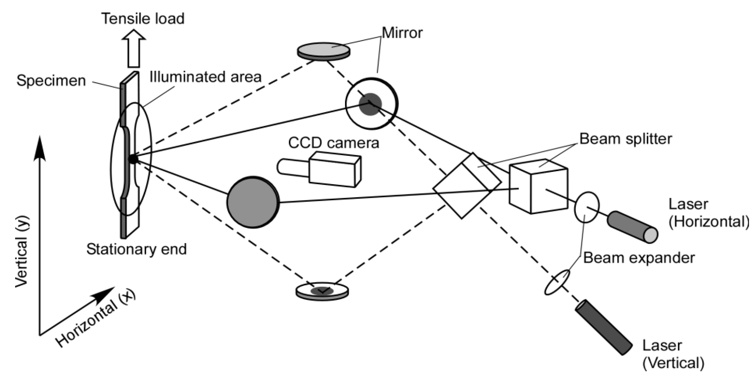
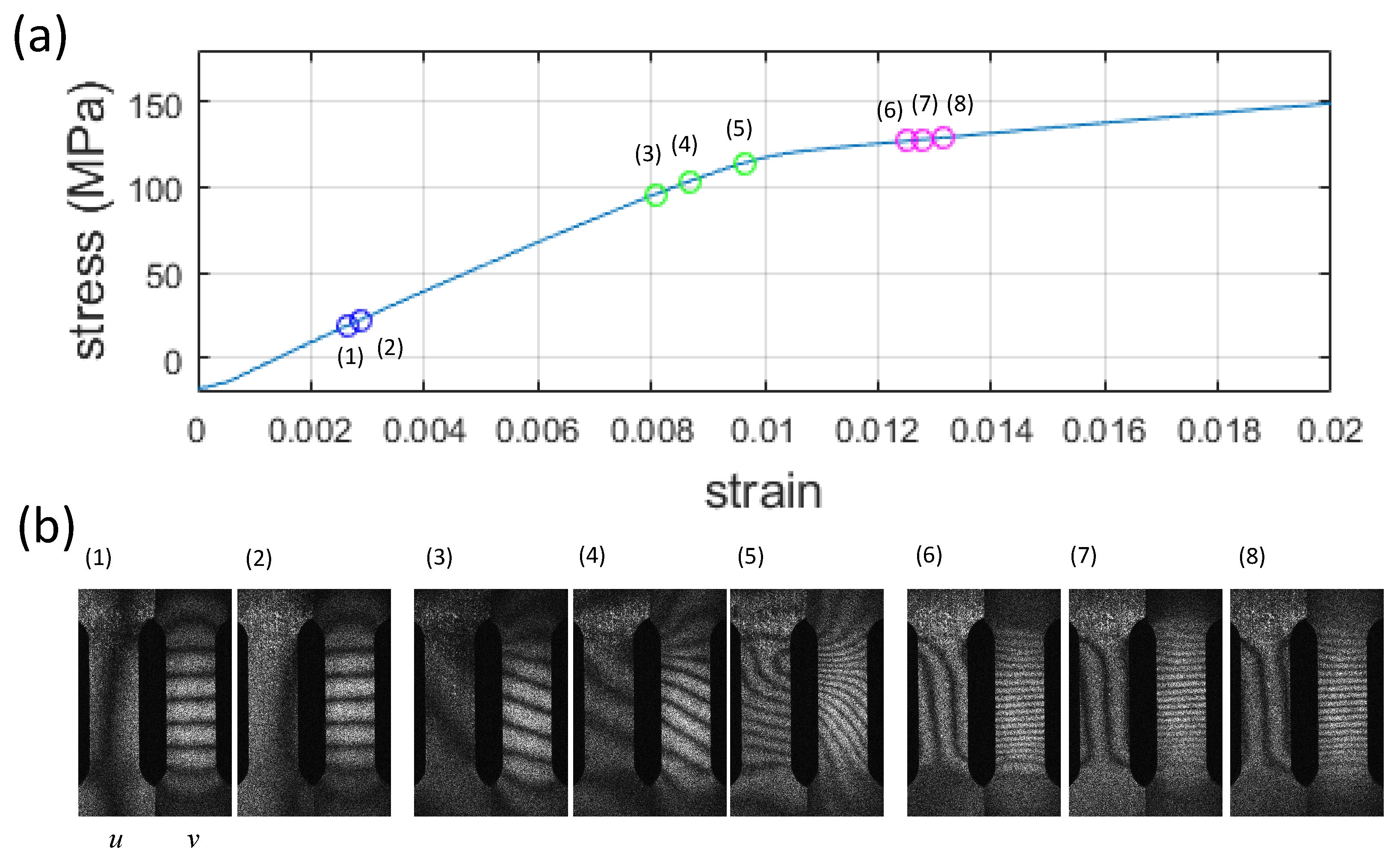
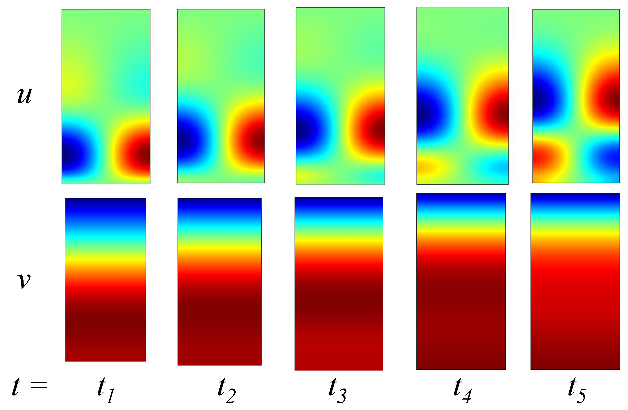
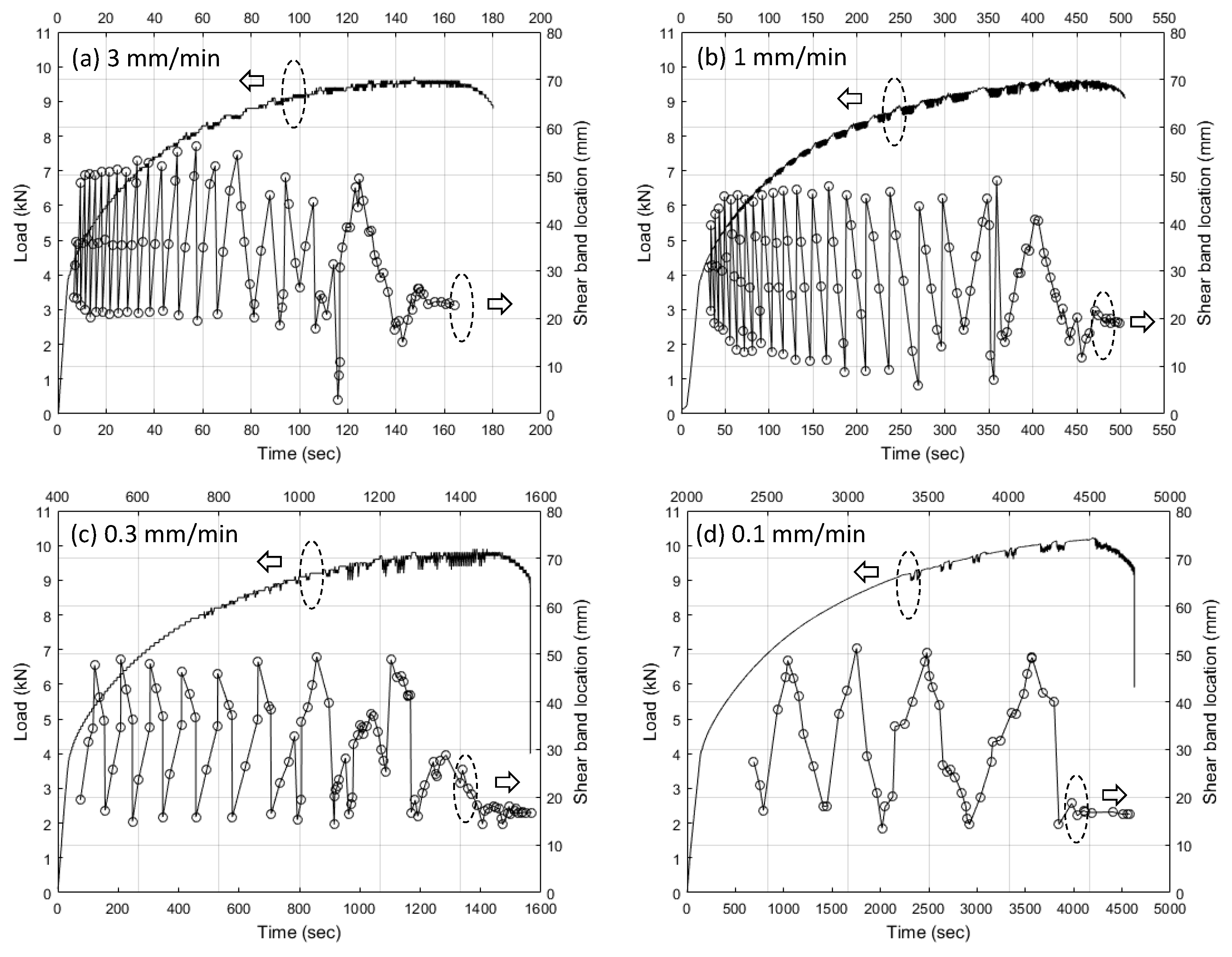
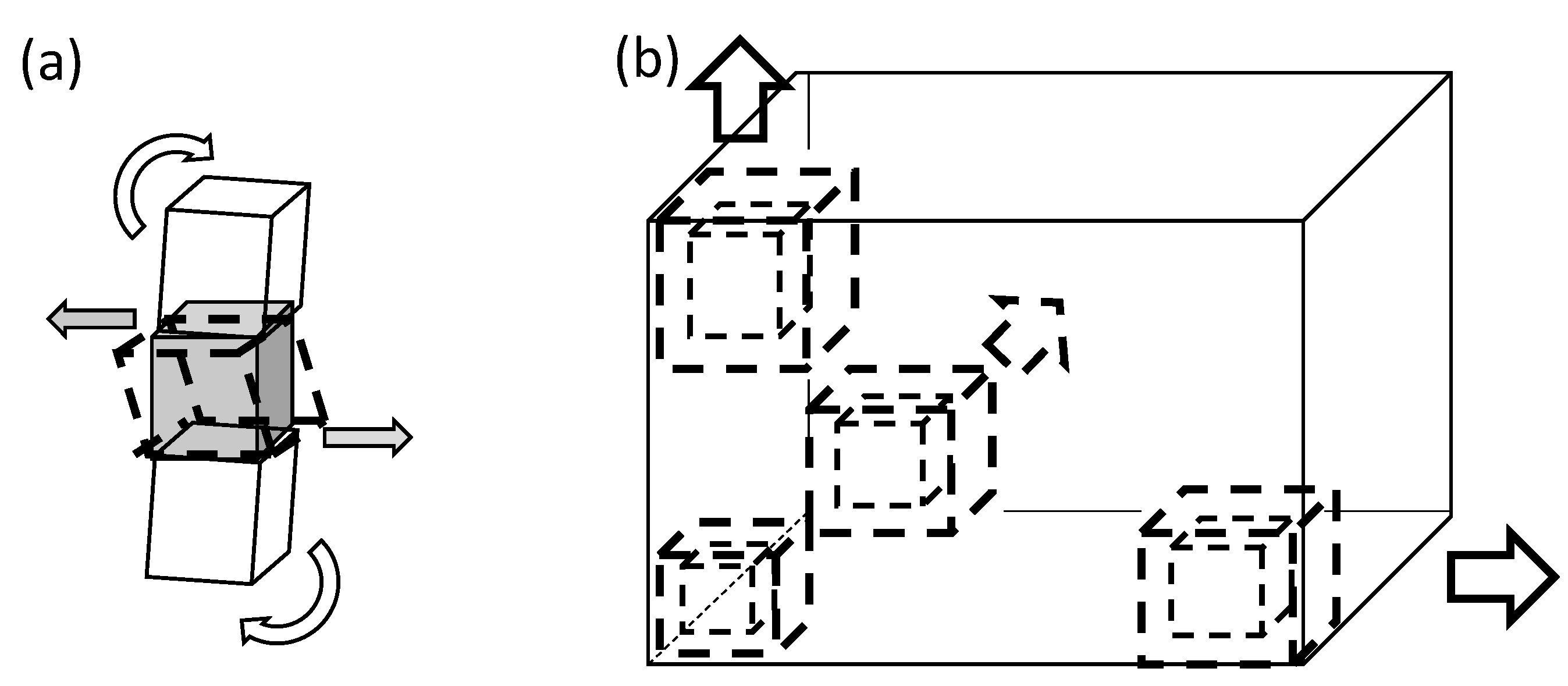
Table 1.
Elastic conditions.
| G (N/m) | (N/m) | (kg/m) | Pulling Rate (m/s) | |||
|---|---|---|---|---|---|---|
| 1 | 0.3 | 1 | 35 |
Table 2.
Various quantities at onset of shear band propagation. Quantities in the top three rows are found directly from experimental data. Quantities in the bottom three rows are evaluated based on theories.
Table 2.
Various quantities at onset of shear band propagation. Quantities in the top three rows are found directly from experimental data. Quantities in the bottom three rows are evaluated based on theories.
| Pulling Rate (mm/min) | 3 | 1 | 0.5 | 0.3 | 0.1 |
|---|---|---|---|---|---|
| Onset time (s) | 6.6 | 31.1 | 150.1 | 456.2 | 2415 |
| Elongation (mm) | 0.55 | 0.51 | 1.25 | 2.28 | 4.02 |
| Normal strain (%) | 2.2 | 2.0 | 5.0 | 9.1 | 16.1 |
| Dislocation velocity (cm/s) | 1.92 | 7.16 | 1.77 | 6.03 | 1.16 |
| Dislocation density (cm) | 3.6 | 3.3 | 6.6 | 1.2 | 2.0 |
| Solitary wave amplitude (mm/min) | 11.5 | 4.29 | 1.06 | 0.36 | 0.07 |
© 2020 by the authors. Licensee MDPI, Basel, Switzerland. This article is an open access article distributed under the terms and conditions of the Creative Commons Attribution (CC BY) license (http://creativecommons.org/licenses/by/4.0/).
Share and Cite
MDPI and ACS Style
Yoshida, S.; McGibboney, C.; Sasaki, T. Nondestructive Evaluation of Solids Based on Deformation Wave Theory. Appl. Sci. 2020, 10, 5524. https://doi.org/10.3390/app10165524
AMA Style
Yoshida S, McGibboney C, Sasaki T. Nondestructive Evaluation of Solids Based on Deformation Wave Theory. Applied Sciences. 2020; 10(16):5524. https://doi.org/10.3390/app10165524
Chicago/Turabian StyleYoshida, Sanichiro, Conor McGibboney, and Tomohiro Sasaki. 2020. "Nondestructive Evaluation of Solids Based on Deformation Wave Theory" Applied Sciences 10, no. 16: 5524. https://doi.org/10.3390/app10165524
Note that from the first issue of 2016, this journal uses article numbers instead of page numbers. See further details here.