Effects of the Top Edge Impedance on Sound Barrier Diffraction

1
Key Laboratory of Modern Acoustics (MOE), Institute of Acoustics, Nanjing University, Nanjing 210093, China
2
NJU-Horizon Intelligent Audio Lab, Nanjing Institute of Advanced Artificial Intelligence, Nanjing 210014, China
3
Centre for Audio, Acoustics and Vibration, Faculty of Engineering and IT, University of Technology Sydney, 2007 Ultimo, Australia
*
Author to whom correspondence should be addressed.
Appl. Sci. 2020, 10(17), 6042; https://doi.org/10.3390/app10176042
Submission received: 31 July 2020
/
Revised: 22 August 2020
/
Accepted: 28 August 2020
/
Published: 31 August 2020
(This article belongs to the Special Issue Noise Barriers)
Abstract
:Sound barriers can be configured with different top edge impedance to improve their noise control performance. In this paper, the integral equation method was used to calculate the sound field of a barrier with various top edge impedance, and the effects of the barrier top edge impedance on sound barrier diffraction were investigated. The simulation results showed that the noise reduction performance of a sound barrier with a soft boundary on its top edge was larger than that with a hard boundary, but there were some impedance values which, if assigned to the top edge boundary, would give the sound barrier even better noise reduction performance. It was found that the sound barrier with a good top edge impedance formed a dipole-like radiation pattern above the barrier to expand the effective range of the shadow zone. The research discoveries reported in this paper point out the potentials of using acoustics metamaterials or active control methods to implement the desired good impedance on the top edge of a sound barrier for better noise reduction.
1. Introduction
Sound barriers have been widely used for the alleviation of noise nuisance in outdoor engineering projects, such as highways [1], railways [2], and high-rise buildings [3]. Although acoustic performance is important for noise barriers, other factors, such as noise source visibility and barriers aesthetics, also need to be considered when designing noise barriers, as they affect the subjective perception of the barrier effectiveness in complex ways [4,5,6,7,8]. Therefore, although the acoustic performance of barriers can be simply improved by increasing the barrier height, this cannot be done in practical applications due to various objective and subjective factors such as cost and visual effects. To improve the acoustic performance of a noise barrier without increasing its height, various types of barrier have been investigated. One type of the new barriers involves modifying the shape of the barrier, and barriers with new profiles, such as T-shape barriers, Y-shape barriers, circular barriers [9], multiple edge barriers [10], and wave-trapping barriers [11] have been designed. Another type involves suppressing the sound pressure at the barrier’s edge by installing an acoustically soft [12] or absorbent material [13]. These two types can be considered simultaneously when designing the barriers. Ishizuka and Fujiwara tested the acoustic performance of noise barriers with various shapes and surface conditions using a two-dimensional Boundary Element Method (BEM), and they found that the absorbing and soft edges improved the efficiency of the barrier significantly and the T-shape design was the most effective in the absorbing and the soft cases [9].
In further improving the acoustic performance, barriers with complex shapes of top devices have attracted a lot of attention. Monazzam and Lam investigated the acoustic performance of noise barriers with quadratic residue diffuser (QRD) tops using a two-dimensional BEM and found that insertion loss produced by utilizing QRD on different barrier profiles varied significantly with frequency and was strongly dependent on the design frequency of the QRD [14]. Later, Naderzadeh et al. found that the diffuser performance could be improved by treating the diffuser with perforated sheets either on the top surface or inside the wells [15]. Okubo and Fujiwara investigated a noise barrier with a Waterwheel cylinder installed on the top edge to improve the sound shielding efficiency of a noise barrier, and the effective range was extended by assigning additional channels corresponding to the ineffective range [16,17]. However, due to the lack of research on the effects of the top edge impedance on the sound barrier diffraction, the barrier performance can only be improved through optimization algorithms [18,19,20]. Besides, some phenomena in prior studies cannot be properly explained, such as findings that barriers with “acoustically soft surface” edge perform better than barriers with “theoretical soft surface” edge in certain frequency bands [21].
To further investigate the effects of top edge impedance on sound barrier diffraction, it is important to accurately calculate the sound field around barriers with arbitrary top edge impedance. The diffraction of waves by a thin half plane has been studied since the 18th century [22]. MacDonald [23] formulated a mathematically rigorous solution to solve generalized diffraction problems by planes due to cylindrical and spherical incident waves, and Hadden and Pierce proposed an analytical model to predict the sound pressure diffracted by a wedge [24]. Besides these two conventional analytical solutions, the geometrical theory of diffraction (GTD) developed by Keller is another commonly used method, which shows that the source of the diffracted rays is determined by the incident rays toward the barrier’s top and an appropriate diffraction coefficient [25]. However, these conventional analytical methods are no longer capable of dealing with the barriers with complex profiles and complex impedances, where the BEM becomes a good option [26,27]. The basic formulation and implementation of a collocation BEM are well established, but they generally consume large amounts of computing resources and errors may arise when performing discretization and solving integrations [28,29].
In addition to the commonly used BEM, Zhao et al. proposed an analytical method for calculating sound field around a rigid noise barrier based on the integral equation method, which requires much less computation resources than the Finite Element Method (FEM) [30]. Based on the same principle, an analytical method for calculating sound field of a barrier with arbitrary top edge impedance was introduced first, and then the effects of top edge impedance on sound barrier diffraction were investigated.
2. Theory
2.1. Theoretical Equation
A two-dimensional sound field was assumed throughout this paper for less computational resources and calculation time. It has already been shown by scale-model experiments that the two-dimensional analyses can be applied to the three-dimensional situation when a point source and a receiver are in the vertical plane which is perpendicular to the barrier [17]. Figure 1 shows the barrier in the free field to be investigated and the coordinate system for solving the problem.
The barrier was assumed to be located at −L/2 < x < L/2, y < 0, where L is the thickness of the barrier. The normal admittance of the top edge B2 was supposed to be β in the following text, where β = 0 denotes the rigid boundary while β = ∞ denotes the soft boundary. Since the purpose of this research was to study the effects of top edge impedance on sound barrier diffraction, barrier front and back surfaces B1 and B3 were assumed to be rigid. A point source S was located at rs = (xs, ys) on the left side of the barrier. The transmission loss of the barrier was supposed to be large enough to ensure that the sound field behind the barrier was only the diffraction wave. The whole space was divided into three subspaces as shown in Figure 1. Space I consisted of the space x < −L/2, y < 0, barrier B1, virtual boundary Σ1, and quadrant C1, where point S indicates the primary source. Space II consisted of the space y > 0, barrier B2, virtual boundary Σ1, Σ2, and quadrant C2. Space III consisted of the space x > L/2, y < 0, barrier B3, virtual boundary Σ2, and quadrant C3. The diameter of C1, C2, and C3 is infinite.
Following the Kirchhoff–Helmholtz equation, the sound field at location r in each of the three subspaces can be described as [31]:
where r′ is the position vector on the boundaries and pi(r) is the sound field generated by the point source, which can be obtained by pi(r) = jωρ0qsG1(r|rs). ω is the angular frequency, ρ0 is the air density, qs is the source strength of the point source, and G1, G2, G3 are the Green functions of the three subspaces, respectively.
The sound field must satisfy the rigid boundary conditions of B1, B3, and impedance boundary condition of B2 simultaneously, namely,
For convenience of calculation, the Green function can be selected so that
which can be obtained with the image method [32] as:
where r′1, r′2, and r′3 are the image location of r′ regarding the corresponding boundaries.
By combining the boundary conditions and the fact that the integration over C1, C2, and C3 tends to be zero with the infinite large diameter [31], Equations (1)–(3) becomes
It can be seen that the sound field is determined by the normal partial derivative of the sound pressure on the boundary ∑1, B2, and ∑2. Using the continuation conditions on the virtual boundary ∑1 and ∑2, namely:
and the boundary condition of B2 shown in Equation (5), it has:
where ,, and are the normal partial derivatives of the sound pressure on ∑1, B2, and ∑2, respectively.
Although the proposed method is a rigorous solution and holds in the whole space, it is hard to solve Equations (15)–(17) analytically, so numerical scheme was utilized. Take N1, N2, and N3 sampling points on ∑1, B2, and ∑2 respectively, then the integral equation can be discretized into matrix form as
where I is the identity matrix, , , and
The normal partial derivative of sound pressure at all sampling points can be obtained by solving Equation (18). Then, the sound field at any location r in the space can be calculated with Equations (10)–(12).
2.2. Verification
Assume the normal admittance of the top edge is β = jβ0tan(kl), where β0 is the characteristic admittance of the air, k is the wave number, and l = 0.1715 m. It is the equivalent acoustic impedance at the opening of a quarter-wave resonator (a well with closed end) resonating at 500 Hz. Fifty sampling points at equal intervals were used on B2, and 800 sampling points at exponential intervals were used on Σ1 and Σ2, respectively. The farthest sampling point was about 10 m from the barrier and the maximum sampling point interval was about 0.034 m. The point source was located at S (−5, −5) m. Figure 2 shows the calculated sound pressure level (SPL) at two receiving points at R1 (2, −2) m and R2 (4, 2) m as well as the results from the commercial software (COMSOL Multiphysics v5.4). The agreement of the two methods at both R1 and R2 was reasonably good, which verifies the reliability of the proposed method.
The SPL curves at two receiving points when the top edge was a rigid boundary (by setting β = 10−10) or a soft boundary (by setting β = 1010) are also given in Figure 2 for comparison. The results of setting the top edge to a rigid boundary or a soft boundary in the COMSOL simulations are consistent with the results of setting β = 10−10 or β = 1010 in the proposed method, respectively. Thus, it was reasonable to set β = 10−10 to simulate the rigid boundary and to set β = 1010 to simulate the soft boundary. The same settings were used for the simulation below. It can be seen that the SPL with β = jβ0tan(kl) was smaller than that of soft boundary in certain frequency band and greater than that of rigid boundary in another frequency band. Because β = jβ0 tan(kl) was the normal admittance at the opening of a well, Figure 2 implies that although installing a well on top edge can improve the barrier performance in a specific frequency band, it reduces the performance in another frequency band below the effective frequency. This is consistent with the phenomenon observed in prior research [21].
3. The Effects of Top Edge Impedance on Sound Barrier Diffraction
3.1. The Good and Bad Top Edge Impedance
The sound power level (SWL) flowing from Σ2 to Space III as a function of the top edge impedance at 500 Hz and 1000 Hz is shown in Figure 3. Negative acoustic resistance (real part of the impedance) implies the introduction of additional acoustic energy, so it was not drawn in the figure. It can be found from the figure that the acoustic resistance corresponding to the peak and valley of the SWL was 0 at these two frequencies, indicating that the “good impedance” and “bad impedance,” which represent the top edge boundary condition corresponding to the minimum and maximum sound power flowing from Σ2 to Space III, were both pure acoustic reactance. Therefore, the top edge resistance was set to 0 in this section, i.e., β was assumed to be an imaginary number.
Figure 4a,b shows the SPL as a function of the imaginary part of top edge admittance at two receiving points at 500 Hz. It can be observed that there were multiple β superior to the soft boundary or worse than the rigid boundary. The good and bad acoustic admittances regarding the sound power flowing from Σ2 to Space III are shown in Figure 4c at 10 frequencies from 100 Hz to 1000 Hz, and corresponding SWLs flowing into the sound shadow zone are shown in Figure 4d. The good and bad admittance values decreased with increasing frequency in general, and the same occurred with the sound power flowing into the sound shadow zone.
3.2. Mechanism Analysis
The good (β = 27.3jβ0) and bad (β = 11.2jβ0) impedances of 500 Hz were used as examples to explain the mechanisms. The normal sound intensity, sound pressure amplitude, normal particle velocity amplitude, and the phase difference between the sound pressure and normal particle velocity at each point on the boundary between the sound shadow zone and the sound bright zone under different boundary conditions are shown in Figure 5. For the rigid case, the sound energy in the sound shadow area mainly flowed from the area within 0.1 m from the top edge because the normal sound intensity at x = 0.1 m was only 1% near the top edge. The effects of different top edge impedance on the diffraction sound field were mainly reflected in the change of the normal sound intensity in this area. The sound pressure in the range of x < 0.1 m for the soft boundary was much less than that for the rigid boundary even though their normal particle velocities were similar, indicating that the control mechanism of the soft boundary was to reduce the sound pressure near the top edge of the barrier. For the bad top edge impedance, both the sound pressure and normal particle velocity were large with a small phase difference, resulting in the largest normal sound intensity. For the good top edge impedance, the normal particle velocity increased but was out of phase (phase difference is larger than π/2) with the sound pressure in the range of x < 0.005, as evidenced by the negative normal sound intensity in this range. The sound pressure in the range of x > 0.005 m was much less than that of the soft case, so normal sound intensity was the minimum.
The SPL and sound intensity distribution near the top edge of the barrier under the four boundary conditions are shown in Figure 6. In Figure 6a,b, when the bad top edge impedance was used, the pressure increased significantly at the top edge and the direction of the sound intensity was nearly parallel to the top edge, which can increase the diffracted sound according to the GTD theory [25]. In Figure 6c, the incident sound wave interfered with the secondary sound wave generated at the top edge, forming a dipole-like radiation above the barrier, so the sound energy radiating into the sound shadow zone was reduced. Compared with the soft boundary sound field shown in Figure 6d, the size of the low sound pressure range at the top of the barrier with the good top edge impedance was larger.
4. A Simple Example of Implementing the Good Top Edge Impedance
According to Section 3, the good top edge impedance can be pure reactance, which can be obtained by digging a well on top of the barrier in a specific frequency band because the theoretical normal admittance at the opening of a well with a depth of l is β = jβ0tan(kl). A model was established in COMSOL, in which the depth of the well was 0.1684 m, and the opening size was consistent with the barrier thickness, which was 0.01 m. The maximum element size was set to 0.048 m, which corresponds to the one-seventh of the acoustic wavelength at 1 kHz, and the minimum element size was set to one-thirtieth the thickness of the barrier.
The SWL flowing from Σ2 to Space III calculated by COMSOL simulation is shown in Figure 7a. The peak value appeared at 482 Hz, and the valley value appeared at 500 Hz. Figure 7b shows the comparison of the equivalent normal admittance at the opening of the well at the peak and valley frequencies of the SWL curve and the theoretical bad and good top edge impedance. Although the equivalent normal admittance at the opening of the well was not uniform, the results at most measurement points agreed roughly with that from the theoretical values.
The sound pressure level and sound intensity distribution near the top edge of the barrier at 482 Hz and 500 Hz are shown in Figure 8a,b, respectively. It can be seen from Figure 8 that the reflected sound wave of the well interfered constructively with the incident wave at 482 Hz, while it interfered destructively with the incident wave at 500 Hz. These two sound field distributions shown in Figure 8 are basically the same as those in Figure 6a,c, indicating that the mechanisms at these two frequencies can be equivalent to obtaining a bad top edge impedance or a good top edge impedance. This shows that the bad and the good top edge impedance can be realized in a certain frequency by digging a well at the top of the barrier.
According to the above results and discussion, the system with good impedance can have larger noise control performance than that with soft boundary. However, the required impedance is frequency-dependent, which is difficult to implement in broadband control with passive materials. Active noise control (ANC) techniques have been used to realize broadband soft boundary near the top edge of the barrier by minimizing the near-field sound pressure [33], and the feasibility of controlling the near-field acoustic impedance has been demonstrated [34]. Future research can use the ANC system to achieve the designed impedance in a broadband frequency range.
5. Conclusions
This paper investigated the effects of the top edge impedance on the noise reduction performance of sound barriers by calculating sound field of a sound barrier with the integral equation method. The accuracy of the integral equation method was validated first using the COMSOL simulations. It was found that there some impedance values existed for the top edge of a barrier which could have better noise reduction performance than that with a soft boundary. The control mechanism of these good top edge impedances was a dipole-like radiation pattern which formed above the barrier, where the normal particle velocity was out of phase with the sound pressure, so the normal sound intensity was the minimum and the size of the low sound pressure zone became larger. The good top edge impedance can be realized in a certain frequency by digging a well at the top of the barrier. Future research includes establishing the relationship between the good top edge impedance and the incident sound wave and the target area, seeking a more intuitive explanation of the mechanisms, and using acoustics metamaterials or active control methods to implement the desired impedance on the top edge of a sound barrier for better noise reduction.
Author Contributions
X.Q. and X.H. initiated and developed the ideas related to this research; X.H. and H.Z. carried out numerical analyses; and all authors contribute to the writing of the paper. All authors have read and agreed to the published version of the manuscript.
Funding
This research was funded by the National Natural Science Foundation of China with the grant numbers 11874218, 11874219.
Conflicts of Interest
The authors declare no conflict of interest.
References
- Hayek, S.I. Mathematical-modeling of absorbent highway noise barriers. Appl. Acoust. 1990, 31, 77–100. [Google Scholar] [CrossRef]
- Morgan, P.A.; Hothersall, D.C.; Chandlerwilde, S.N. Influence of shape and absorbing surface—A numerical study of railway noise barriers. J. Sound Vib. 1998, 217, 405–417. [Google Scholar] [CrossRef]
- Tang, S.K. Noise screening effects of balconies on a building facade. J. Acoust. Soc. Am. 2005, 118, 213–221. [Google Scholar] [CrossRef] [PubMed]
- Arenas, J.P. Potential problems with environmental sound barriers when used in mitigating surface transportation noise. Sci. Total Environ. 2008, 405, 173–179. [Google Scholar] [CrossRef] [PubMed]
- Jiang, L.; Kang, J. Combined acoustical and visual performance of noise barriers in mitigating the environmental impact of motorways. Sci. Total Environ. 2016, 543, 52–60. [Google Scholar] [CrossRef] [PubMed] [Green Version]
- Aylor, D.E.; Marks, L.E. Perception of noise transmitted through barriers. J. Acoust. Soc. Am. 1976, 59, 397–400. [Google Scholar] [CrossRef]
- Joynt, J.L.R.; Kang, J. The influence of preconceptions on perceived sound reduction by environmental noise barriers. Sci. Total Environ. 2010, 408, 4368–4375. [Google Scholar] [CrossRef] [Green Version]
- Maffei, L.; Masullo, M.; Aletta, F.; Gabriele, M.D. The influence of visual characteristics of barriers on railway noise perception. Sci. Total Environ. 2013, 445–446, 41–47. [Google Scholar] [CrossRef]
- Ishizuka, T.; Fujiwara, K. Performance of noise barriers with various edge shapes and acoustical conditions. Appl. Acoust. 2004, 65, 125–141. [Google Scholar] [CrossRef]
- Watts, G.R.; Crombie, D.H.; Hothersall, D.C. Acoustic performance of new designs of traffic noise barriers: Full scale tests. J. Sound Vib. 1994, 177, 289–305. [Google Scholar] [CrossRef]
- Yang, C.; Pan, J.; Cheng, L. A mechanism study of sound wave-trapping barriers. J. Acoust. Soc. Am. 2013, 134, 1960–1969. [Google Scholar] [CrossRef] [PubMed] [Green Version]
- Wang, Y.; Jiao, Y.; Chen, Z. Research on the well at the top edge of noise barrier. Appl. Acoust. 2018, 133, 118–122. [Google Scholar] [CrossRef]
- Fujiwara, K.; Furuta, N. Sound shielding efficiency of a barrier with a cylinder at the edge. Noise Control Eng. J. 1991, 37, 5. [Google Scholar] [CrossRef]
- Monazzam, M.R.; Lam, Y.W. Performance of profiled single noise barriers covered with quadratic residue diffusers. Appl. Acoust. 2005, 66, 709–730. [Google Scholar] [CrossRef] [Green Version]
- Naderzadeh, M.; Monazzam, M.R.; Nassiri, P.; Fard, S.M.B. Application of perforated sheets to improve the efficiency of reactive profiled noise barriers. Appl. Acoust. 2011, 72, 393–398. [Google Scholar] [CrossRef]
- Okubo, T.; Fujiwara, K. Efficiency of a noise barrier with an acoustically soft cylindrical edge for practical use. J. Acoust. Soc. Am. 1999, 105, 3326–3335. [Google Scholar] [CrossRef]
- Okubo, T.; Fujiwara, K. Efficiency of a noise barrier on the ground with an acoustically soft cylindrical edge. J. Sound Vib. 1998, 216, 771–790. [Google Scholar] [CrossRef]
- Baulac, M.; Defrance, J.; Jean, P. Optimisation with genetic algorithm of the acoustic performance of T-shaped noise barriers with a reactive top surface. Appl. Acoust. 2008, 69, 332–342. [Google Scholar] [CrossRef]
- Kim, K.; Yoon, G.H. Optimal rigid and porous material distributions for noise barrier by acoustic topology optimization. J. Sound Vib. 2015, 339, 123–142. [Google Scholar] [CrossRef]
- Duhamel, D. Shape optimization of noise barriers using genetic algorithms. J. Sound Vib. 2006, 297, 432–443. [Google Scholar] [CrossRef]
- Fujiwara, K.; Hothersall, D.C.; Kim, C. Noise barriers with reactive surfaces. Appl. Acoust. 1998, 53, 255–272. [Google Scholar] [CrossRef]
- Li, K.M.; Wong, H.Y. A review of commonly used analytical and empirical formulae for predicting sound diffracted by a thin screen. Appl. Acoust. 2005, 66, 45–76. [Google Scholar] [CrossRef]
- MacDonald, H.M. A class of diffraction problems. Proc. London Math. Soc. 1915, 2, 410–427. [Google Scholar] [CrossRef] [Green Version]
- Hadden, W.J.; Pierce, A.D. Sound diffraction around screens and wedges for arbitrary point source locations. J. Acoust. Soc. Am. 1981, 69, 1266–1276. [Google Scholar] [CrossRef]
- Keller, J.B. Geometrical theory of diffraction. J. Opt. Soc. Am. 1962, 52, 116–130. [Google Scholar] [CrossRef] [PubMed]
- Seznec, R. Diffraction of sound around barriers: Use of the boundary elements technique. J. Sound Vib. 1980, 73, 195–209. [Google Scholar] [CrossRef]
- Piacentini, A.; Invernizzi, M.; Pannese, L. Computational acoustics: Noise reduction via diffraction by barriers with different geometries. Comput. Meth. Appl. Mech. Eng. 1996, 130, 81–91. [Google Scholar] [CrossRef]
- Chevret, P.; Chatillon, J. Implementation of diffraction in a ray-tracing model for the prediction of noise in open-plan offices. J. Acoust. Soc. Am. 2012, 132, 3125–3137. [Google Scholar] [CrossRef]
- Treeby, B.E.; Pan, J. A practical examination of the errors arising in the direct collocation boundary element method for acoustic scattering. Eng. Anal. Bound. Elem. 2009, 33, 1302–1315. [Google Scholar] [CrossRef] [Green Version]
- Zhao, S.; Qiu, X.; Cheng, J. An integral equation method for calculating sound field diffracted by a rigid barrier on an impedance ground. J. Acoust. Soc. Am. 2015, 138, 1608–1613. [Google Scholar] [CrossRef]
- Cheng, J. The Principle of Acoustics, Chinese ed; Science Press: Beijing, China, 2012. [Google Scholar]
- Allen, J.B.; Berkley, D.A. Image method for efficiently simulating small-room acoustics. J. Acoust. Soc. Am. 1979, 65, 943–950. [Google Scholar] [CrossRef]
- Berkhoff, A.P. Control strategies for active noise barriers using near-field error sensing. J. Acoust. Soc. Am. 2005, 118, 1469–1479. [Google Scholar] [CrossRef]
- Zhu, H.; Rajamani, R.; Stelson, K.A. Active control of acoustic reflection, absorption, and transmission using thin panel speakers. J. Acoust. Soc. Am. 2003, 113, 852–870. [Google Scholar] [CrossRef] [PubMed] [Green Version]
Figure 1.
The schematic diagram of the barrier system.
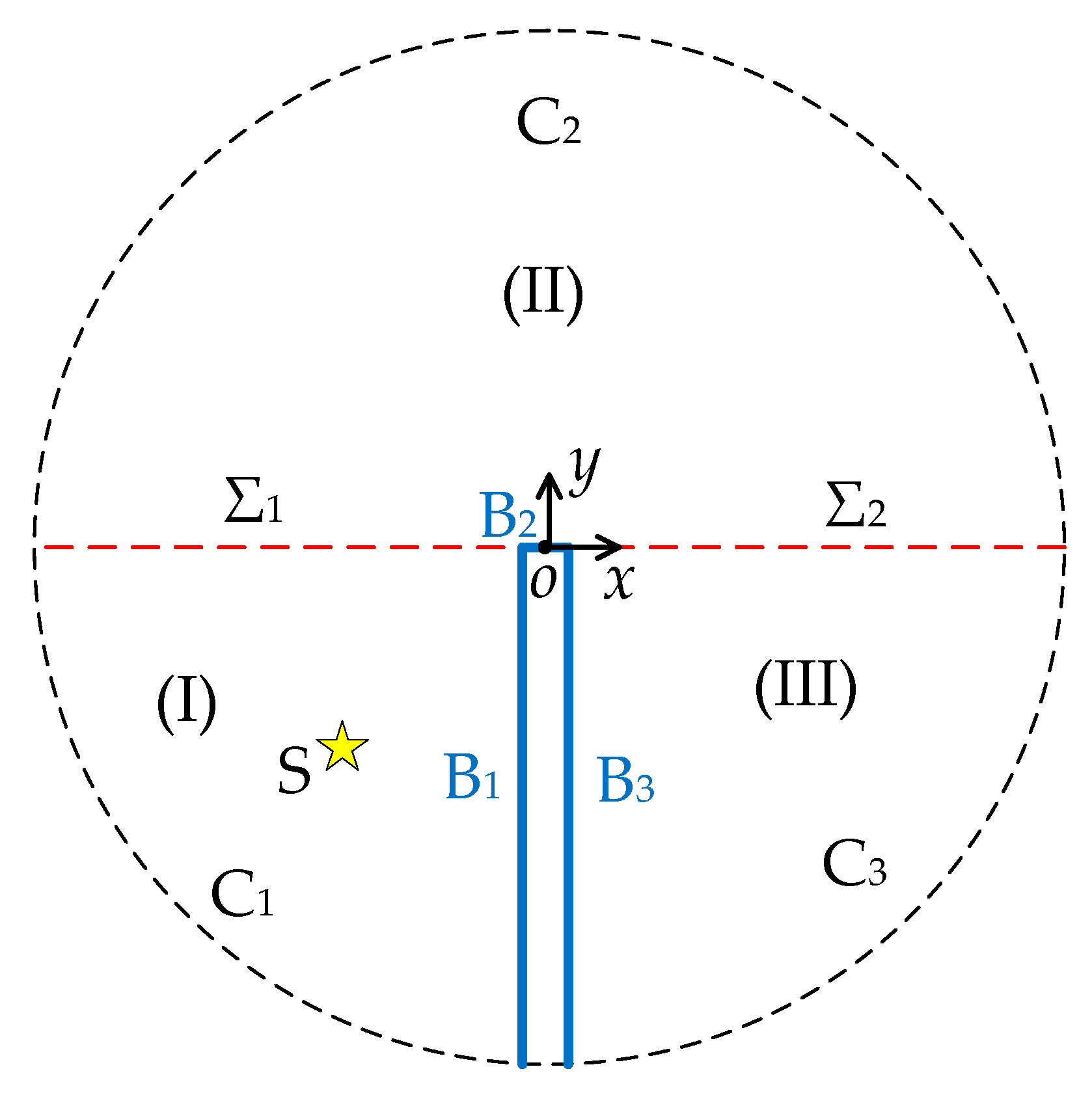
Figure 2.
The sound pressure level (SPL) curve at (a) R1 and (b) R2 with different top edge impedance.
Figure 2.
The sound pressure level (SPL) curve at (a) R1 and (b) R2 with different top edge impedance.

Figure 3.
The sound power level (SWL) flowing from Σ2 to Space III varies with the top edge impedance at (a) 500 Hz; (b) 1000 Hz.
Figure 3.
The sound power level (SWL) flowing from Σ2 to Space III varies with the top edge impedance at (a) 500 Hz; (b) 1000 Hz.
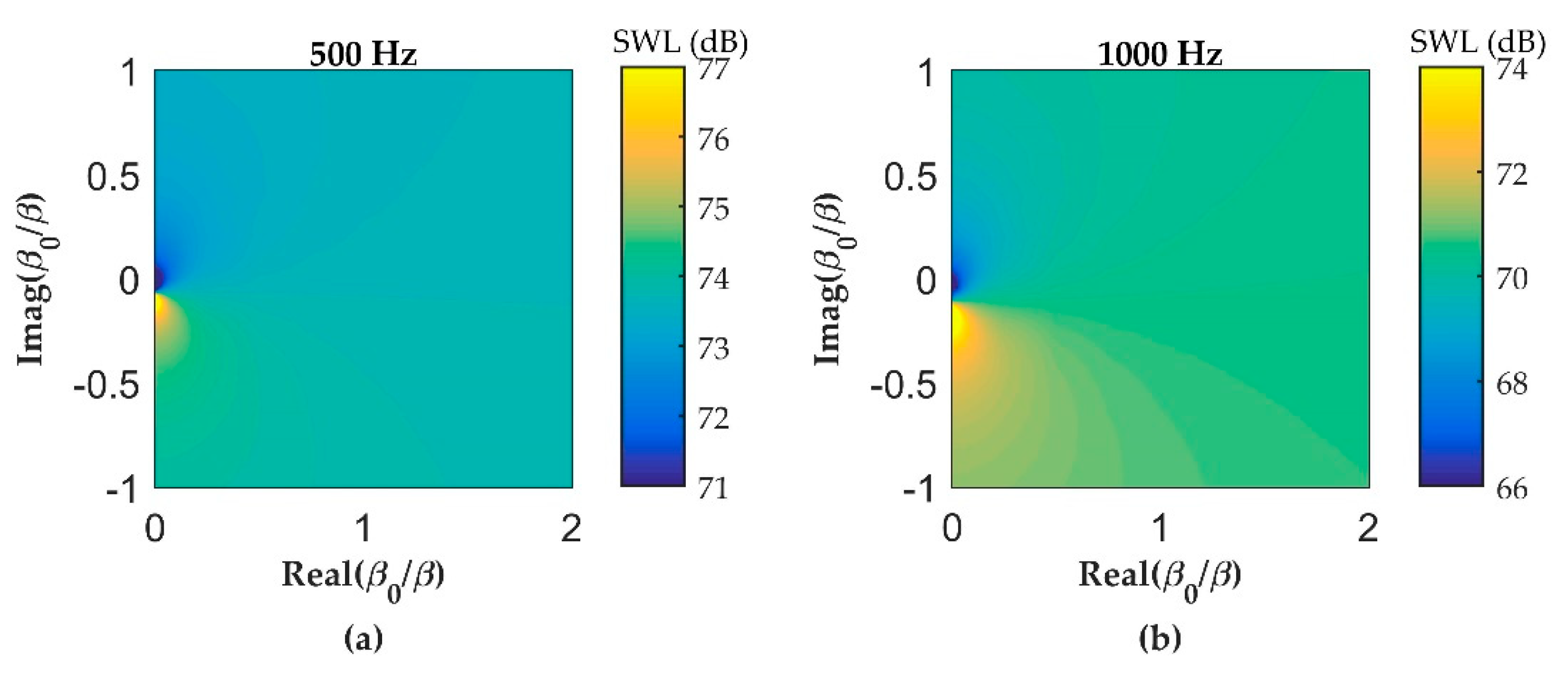
Figure 4.
The good and bad top edge impedance: (a) The SPL curve at R1 as a function of the imaginary part of top edge admittance; (b) the SPL curve at R2 as a function of the imaginary part of top edge admittance; (c) the good and bad top edge impedance regarding the sound power flowing from Σ2 to Space III; (d) the SWL flowing into the sound shadow zone under different boundary conditions.
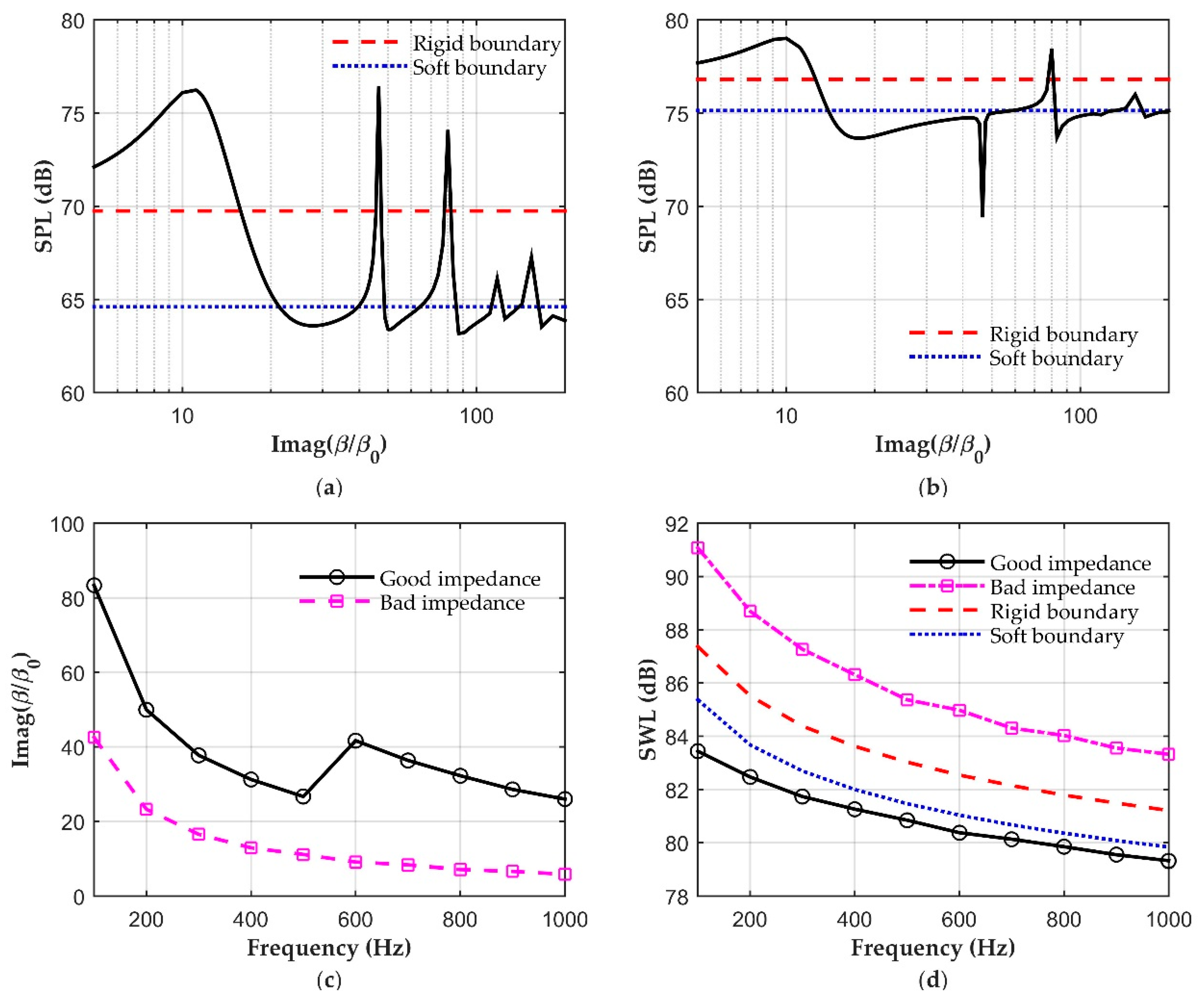
Figure 5.
The physical quantity on the boundary between the sound shadow zone and the sound bright zone: (a) The normal sound intensity; (b) the sound pressure amplitude; (c) the normal particle velocity amplitude; (d) the phase difference between the sound pressure and normal particle velocity, where bad impedance is for β = 11.2jβ0, rigid boundary is for β = 10−10, good impedance is for β = 27.3jβ0 and soft boundary is for β = 1010.
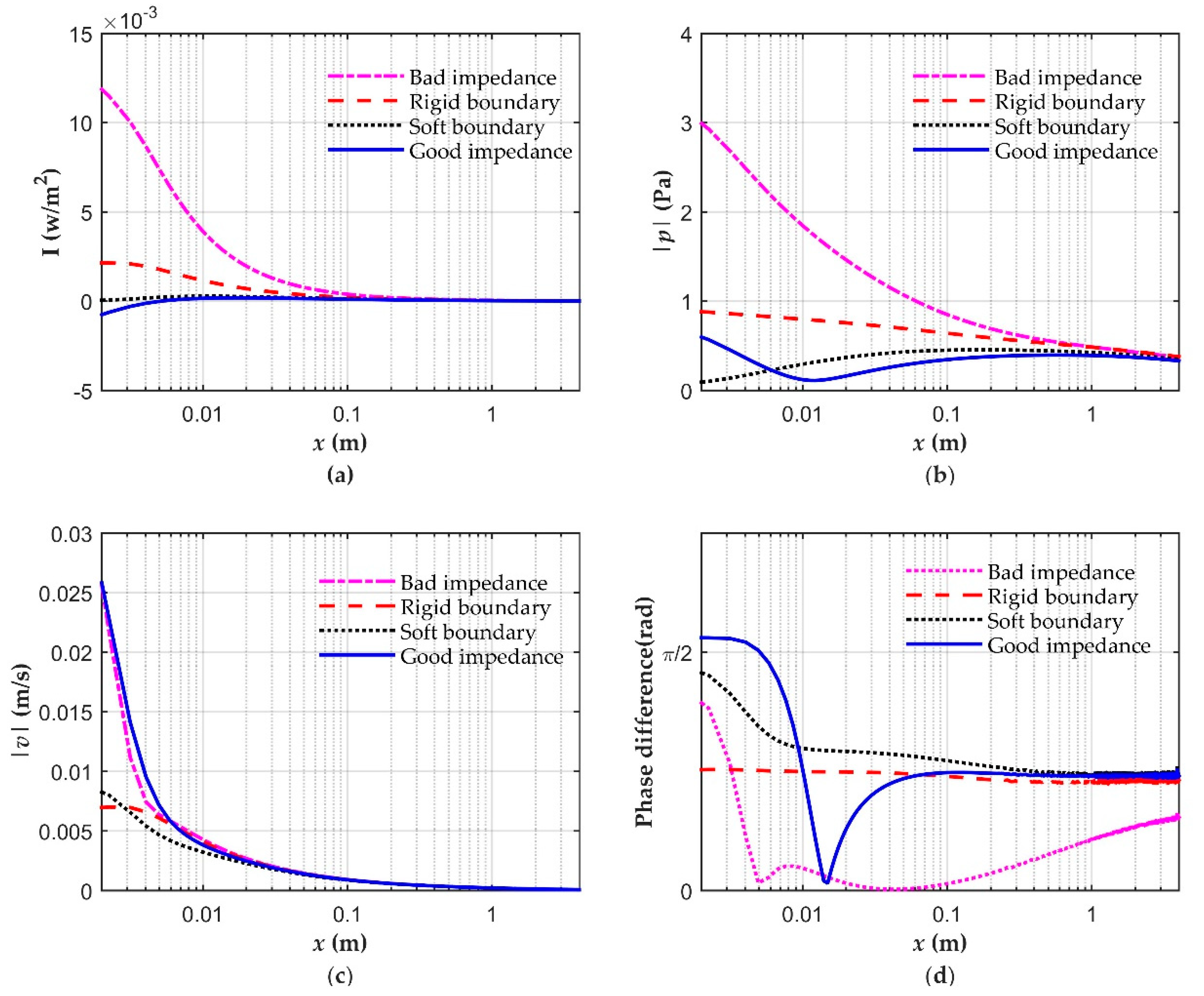
Figure 6.
The SPL and sound intensity distribution at 500 Hz near the top edge of the barrier with (a) bad impedance (β = 11.2jβ0), (b) rigid boundary (β = 10−10), (c) good impedance (β = 27.3jβ0) and (d) soft boundary (β = 1010).
Figure 6.
The SPL and sound intensity distribution at 500 Hz near the top edge of the barrier with (a) bad impedance (β = 11.2jβ0), (b) rigid boundary (β = 10−10), (c) good impedance (β = 27.3jβ0) and (d) soft boundary (β = 1010).

Figure 7.
(a) The SWL flowing from Σ2 to Space III; (b) the equivalent normal admittance at the opening of the well, where bad impedance is for β = 11.2jβ0 and good impedance is for β = 27.3jβ0.
Figure 7.
(a) The SWL flowing from Σ2 to Space III; (b) the equivalent normal admittance at the opening of the well, where bad impedance is for β = 11.2jβ0 and good impedance is for β = 27.3jβ0.
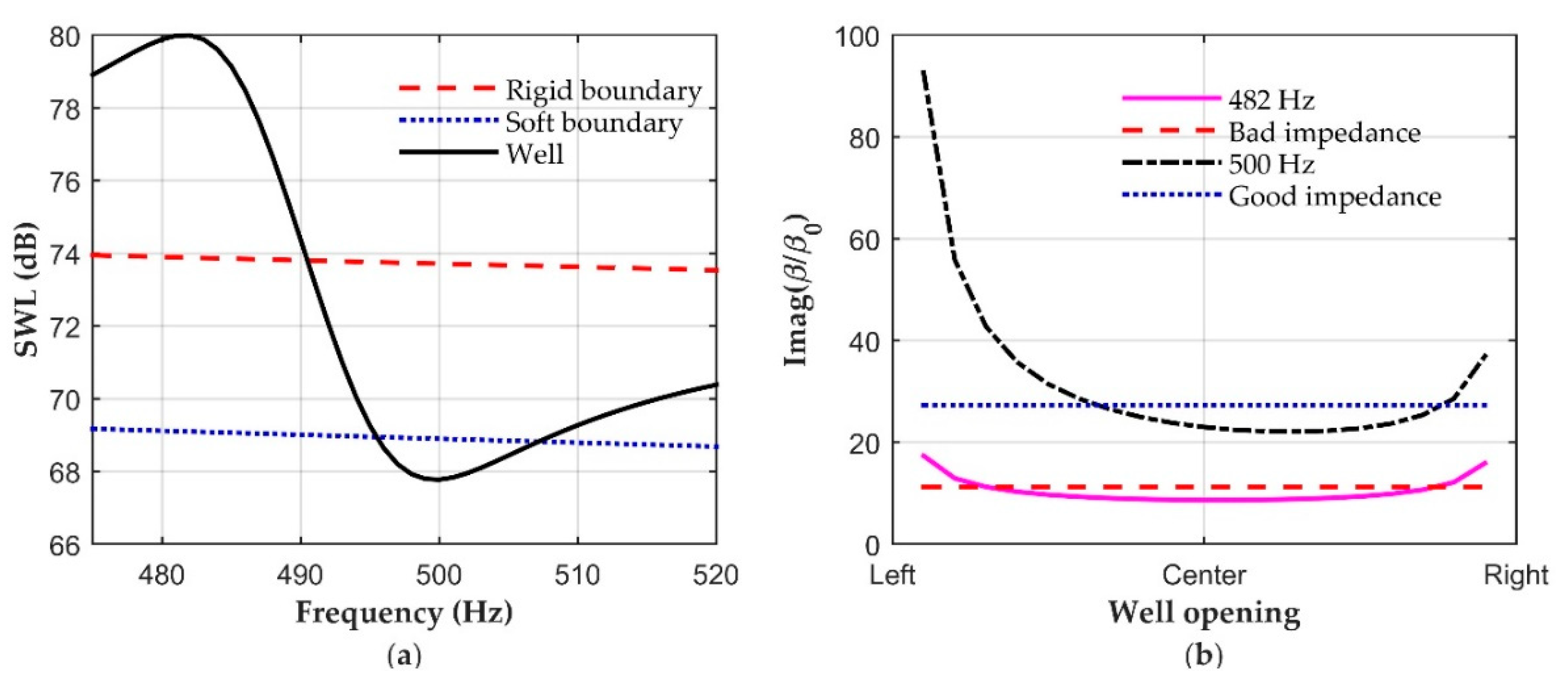
Figure 8.
The SPL and sound intensity distribution near the top edge of the barrier at (a) 482 Hz, (b) 500 Hz.
Figure 8.
The SPL and sound intensity distribution near the top edge of the barrier at (a) 482 Hz, (b) 500 Hz.

© 2020 by the authors. Licensee MDPI, Basel, Switzerland. This article is an open access article distributed under the terms and conditions of the Creative Commons Attribution (CC BY) license (http://creativecommons.org/licenses/by/4.0/).
Share and Cite
MDPI and ACS Style
Huang, X.; Zou, H.; Qiu, X. Effects of the Top Edge Impedance on Sound Barrier Diffraction. Appl. Sci. 2020, 10, 6042. https://doi.org/10.3390/app10176042
AMA Style
Huang X, Zou H, Qiu X. Effects of the Top Edge Impedance on Sound Barrier Diffraction. Applied Sciences. 2020; 10(17):6042. https://doi.org/10.3390/app10176042
Chicago/Turabian StyleHuang, Xiaofan, Haishan Zou, and Xiaojun Qiu. 2020. "Effects of the Top Edge Impedance on Sound Barrier Diffraction" Applied Sciences 10, no. 17: 6042. https://doi.org/10.3390/app10176042
Note that from the first issue of 2016, this journal uses article numbers instead of page numbers. See further details here.