World-Models for Bitrate Streaming


Computer Laboratory, University of Cambridge, Cambridge CB3 0FD, UK
*
Author to whom correspondence should be addressed.
Appl. Sci. 2020, 10(19), 6685; https://doi.org/10.3390/app10196685
Submission received: 18 August 2020
/
Revised: 17 September 2020
/
Accepted: 18 September 2020
/
Published: 24 September 2020
(This article belongs to the Special Issue AI in Mobile Networks)
Abstract
:Adaptive bitrate (ABR) algorithms optimize the quality of streaming experiences for users in client-side video players, especially in unreliable or slow mobile networks. Several rule-based heuristic algorithms can achieve stable performance, but they sometimes fail to properly adapt to changing network conditions. Fluctuating bandwidth may cause algorithms to default to behavior that creates a negative experience for the user. ABR algorithms can be generated with reinforcement learning, a decision-making paradigm in which an agent learns to make optimal choices through interactions with an environment. Training reinforcement learning algorithms for bitrate streaming requires building a simulator for an agent to experience interactions quickly; training an agent in the real environment is infeasible due to the long step times in real environments. This project explores using supervised learning to construct a world-model, or a learned simulator, from recorded interactions. A reinforcement learning agent that is trained inside of the learned model, rather than a simulator, can outperform rule-based heuristics. Furthermore, agents that are trained inside the learned world-model can outperform model-free agents in low sample regimes. This work highlights the potential for world-models to quickly learn simulators, and to be used for generating optimal policies.
1. Introduction
Determining bitrates for a positive user experience in unreliable or slow mobile networks can be difficult. Hardcoded algorithms may fail to accurately predict future bandwith, which leads to rebuffering, and users may prefer minimal levels of quality fluctuations. An unreliable network may cause algorithms to select the lowest quality by default; selecting the highest level that bandwidth can support may not satisfy user preferences. Existing computer systems tackling this and other related problems typically make decisions that are based on heuristics in the form of configuration parameters or human-engineered algorithms. However, humans may lack the intuition to tune parameters or design decision-making algorithms. Reinforcement learning is a machine learning paradigm, where an agent can learn to make optimal decisions through interactions with an environment. The reinforcement learning paradigm has been successfully applied to bitrate streaming in the Pensieve project, outperforming rule-based approaches [1]. However, many reinforcement learning algorithms have high sample-complexity, requiring tens of millions of interactions with the real environment to learn an optimal policy. Training these algorithms can be severely constrained by the run time and lack of parallelization in real systems environments. Human-engineered simulators, such as a simulator for bitrate streaming, can replace real environments for training. However, building simulators may require significant developer effort in order to represent the complexities of the environment. Typically, the reinforcement learning algorithms that are applied in practice are model-free; while these algorithms learn a policy to make optimal decisions, they do not learn the dynamics of the environment [2]. Conversely, model-based algorithms learn a model of how the environment will behave, and then use the learned model to derive a policy [3]. World-models are a type of model-based reinforcement learning, where a learned model can simulate all aspects of the environment [4]. Recent work [5,6] has shown that it is possible to train agents entirely inside learned world-models of complex environments, rather than the real environments themselves. Successfully learning world-models could provide vast benefits: cheap parallel training, faster training times, safe experimentation, and increased performance through planning. This work explores whether it is possible to build world-models for bitrate streaming, and whether world-models can provide any benefits in learning optimal policies. We provide experiments that show the performance of an agent trained entirely inside a learned world-model and provide sample complexity comparisons with current model-free algorithms. It demonstrates that world-models can successfully learn simulators from recorded data and world-models can outperform model-free approaches in low sample regimes.
2. Background
2.1. Bitrate Streaming
Streaming video over variable-bandwidth networks requires a client to adapt to network conditions in order to create the optimal user experience [7]. Users like to have high video quality, minimal buffer pauses, and no noticeable differences in quality between video chunks; these preferences vary between users and situations. HTTP-based adaptive streaming, through standards, such as DASH [8], is the predominant form of network streaming today. In DASH, videos are stored on servers in multiple chunks, each holding a few seconds of video. A client-side application makes requests to download chunks, allowing for servers to have stateless backends. Each chunk is encoded at several discrete bitrates, with higher bitrates containing higher resolution and chunk sizes. Quality-of-Experience (QoE) is the primary metric for evaluating the performance of the client. A variety of QoE metrics exist, and many metrics are a function of three factors: maximal resolution, buffering time, and smoothness (rapid changing of bitrates across consecutive chunks) [1]. Selecting the optimal bitrate is challenging, due to the variability of network conditions [9] and the conflicting QoE requirements. Moreover, bitrate decisions can have a cascading effect on QoE over the course of the video; for example, a high bitrate may drain the playback buffer, which causes the video to rebuffer in the future [1]. The QoE metric is defined below for a video of N chunks:
Here, is the chosen bitrate, is a quality function on the chosen bitrate, is a parameter constant, is the time to download the chunk, and the final term is the penalty for consecutive changes in resolution. There are various heuristic-based algorithms for bitrate control. RobustMPC [10], for example, decides the next bitrate by maximizing QoE across the predicted future bitrates in a near horizon, computed through a harmonic mean; however, it can conservatively estimate throughput and requires tuning. Heuristics, such as MPC, may perform extremely poorly when their network assumptions are violated [1]. Pensieve [1] was the first formulation of bitrate streaming as a reinforcement learning problem and it achieved state-of-the-art results on the problem, outperforming human-engineered heuristics, including RobustMPC [10], BOLA [11], and buffer-based [12] algorithms.
2.2. Reinforcement Learning
Reinforcement learning is a decision making paradigm. In reinforcement learning, an agent takes actions in an environment to optimize a cumulative reward. Reinforcement learning problems can be stated as a Markov Decision Process, being formally defined with a four-tuple:
- is the set of possible states;
- is the set of possible actions available to an agent;
- is the transition kernel for states and actions, the probability that an action a at state s leads to state ; and,
- is the reward function, the immediate reward from transitioning to state from s due to action a.
A policy , produces an action a given current state s: . The objective of a reinforcement learning algorithm is to learn a policy that maximizes the expected return in an environment.
Here, is the reward given by the policy selecting action a at time t and is the discount factor that determines the importance of future rewards. For , if the environment does not contain a terminal state, or the agent never reaches one, rewards can become infinite. Typically, reinforcement learning algorithms are evaluated in their performance across episodes, sequences of actions that end with a terminal state. Initially, agents do not have any knowledge of environments; agents must balance between the exploration of unseen states and exploitation of current knowledge to find an optimal policy.
Partially Observable Markov Decision Processes (POMDPs) are MDPs where the state space may be noisy or not fully observable. Reinforcement learning is concerned with learning a policy when the environment model is not known in advance. There are two broad classes of reinforcement learning algorithms: model-free and model-based [3]. Generally, model-free methods learn a policy without learning a model of environment dynamics, and model-based methods learn a model of environment dynamics and use the learned model for deriving a controller. In practice, there are no distinct boundaries between these two classes, and some algorithms blur the lines between the categories [13]. Classical reinforcement learning methods can be untenable on large state and action spaces; the state space may be too large for the agent to visit exhaustively, and there are large memory overheads for dynamic programming methods. Deep reinforcement learning has been used in order to achieve state-of-the-art results on tasks that were previously computationally prohibitive, such as Atari games [14] and Go, a complex board game [15]. Agents that are trained with deep reinforcement learning can learn complex functions, handle unstructured environment data, and predict quality actions in states that have never been visited. There are a wide variety of reinforcement learning algorithms with different use cases and advantages, such as parallelization or properly handling discrete action spaces. Actor-critic methods [16] have achieved recent success on Atari games, StarCraft [17], and visual navigation [18], among others. In actor-critic algorithms, a critic network estimates a value-function, and an actor network updates a policy-network that is based on the estimations from the critic [19]. This work uses the A2C algorithm, a synchronous version of the A3C algorithm. For brevity, this work omits the mathematical details of the A2C algorithm, and it refers the reader to the original A3C paper [16] for more information.
2.3. Motivation for World-Models
Model-free reinforcement learning is notoriously sample inefficient; agents may require tens or hundreds of millions of interactions to learn complex tasks. Rainbow, which is a combination of six extensions to the DQN algorithm, achieved state-of-the-art results for sample efficiency, but it still required 44 million frames to beat existing baselines in the Arcade Learning Environment [20]. Most current reinforcement learning research is evaluated on simulators, games in the Arcade Learning Environment, or other video games. While these control problems may be complex and challenging, one interaction with the environment is typically sub-second. Conversely, many real-world systems can take several seconds to execute one step. Custom-built simulators are often necessary for successfully trainkng reinforcement learning agents in these settings. For example, a simulator for bit-rate streaming can allow an A3C-based agent to experience 100 h of video in only 10 min. of training time [1]. In contrast, training the same agent on the real system would take more than 10 years to receive enough experience to reach comparable performance [7]. Building simulators may be difficult; custom simulators require developer effort and domain knowledge, and built simulators may not accurately model real-world systems [21]. Some reinforcement learning methods that require high sample complexity, such as policy gradient methods, cannot be used if the real environment’s interactions take too long or the simulator is too slow [22]. If one can learn a world-model from recorded data, then one could train an agent inside the world-model without ever interacting with the real system. Agents can train cheaply in parallel with learned models. A learned environment can execute steps without waiting in real-time for real-world events, rendering states, or completing computations that are unrelated to essential aspects of the environment.
3. World-Models
Model-based RL encompasses a wide variety of methods, including world-models. In this project, world-models refer to models of the environment that can be fully substituted in place of the real environment. Some instances of model-based learning may learn the components for a full world-model, but they may not use the model to replace the real environment for training. World-models typically involve two components, the model of the environment, M, and a controller, C [4]. A model learns from real interactions with an environment, and these interactions must be gathered from a controller or logs of previous interactions. A world-model must learn to predict the next state and reward , given the current state s and action a. M can be substituted in place of the real environment as a world-model once a world-model has learned . Figure 1 shows a visualization of a world-model pipeline. First, a world-model is learned from recorded observations. A controller then learns inside the world-model’s hallucinated episodes of the real environment, which can be transferred back to the real environment during deployment. A controller may learn policies fully inside of the world-model [6], use the world-model for planning [23], or use a world-model to augment the real environment [5]. Neural networks can be used as function approximators for modeling the environment. In deterministic, predictable environments, feedforward neural networks can approximate the world-model. However, these networks tend to fail in POMDP problems [24]. Memories of previous events can assist with the difficulties of POMDPs. The Recurrent Neural Network (RNN) architecture is a class of neural network models that process temporal data. The following subsection provides an overview of the RNN architecture.
3.1. Generative Models
RNNs can recognize patterns with dynamic temporal behavior and, thus, serve as the foundation for many world-models. At each step t, a simple recurrent neural network accepts an input , and outputs a value . The RNN passes information from one step of the network to the next. The left side of Figure 2 displays the recurrent nature of an RNN and the right displays an unfolded version of a simple RNN. More complex architectures are used in practice; Hochreiter et al. [25] introduced Long Short-Term Memory (LSTM), a variant of the RNN that was designed to handle long term dependencies in input sequences.
The output of an RNN is deterministic; however, an RNN can output the parameters for probabilistic model to introduce stochasticity [26]. The output distribution is dependent on the hidden state in the RNN, a representation of previous inputs. Mixture Density Networks (MDNs) [27] are a class of models that output the parameters to a Gaussian Mixture Model (GMM), a probabilistic model that is composed of several Gaussian distributions with different weights. GMMs contain three parameters: , the centers of each component, the scales of each component, and , the weights of each component. Rather than performing a regression, this model maximizes the likelihood that a model gives rise to a set of data points. This model can, in theory, approximate any arbitrary continuous probability distribution. Graves [26] combined a Mixture Density Network with an RNN (MDN-RNN), and used the network to achieve state-of-the-art results on handwriting generation. In a prediction network, the hidden state of the model passes through another layer, outputting the parameters to a mixture model , a distribution modeling the input at the next time step. During inference, a sample from the mixture model, is then fed as the next input into the network. This structure allows for a RNN to generate entire sequences, where each output is conditioned on a representation of past states.
3.2. MDN-RNN World-Model
Ha & Schmidhuber [5] used the MDN-RNN to create a hallucinogenic world-model in reinforcement learning environments, achieving state-of-the-art results on the Car Racing and VizDoom tasks. Their work is the primary inspiration for the work in this paper. The Car Racing and VizDoom tasks are stochastic, and a stochastic input process, the network bandwidth, partially determine the bitrate streaming environment. The MDN-RNN can handle random discrete events, such as a monster shooting a fireball in VizDoom. While sampling in MDN-RNN is probabilistic, it can still form approximations for deterministic properties. The MDN-RNN can fit naturally to bitrate streaming, as bitrate streaming contains discrete events, such as bandwidth dropping while passing through a tunnel.
Ha & Schmidhuber [5] first used a variational autoencoder to compress the state space s into a latent vector z, and learned a world model with this compressed version of the state space. The authors train an MDN-RNN to model , where is the action take at time t, is the state of the environment that is encoded as a latent vector at time t, and is the hidden state of the MDN-RNN at time t. The world model is trained using recorded episodes in the teacher forcing method, where the inputs to the MDN-RNN model in training only consist of the ground truth at each step. Sampling only occurs during the training of the controller. For inference, the MDN-RNN uses a softmax layer on the output ’s to form a categorical distribution. The softmax function, , converts a vector of numbers into a probability distribution, where each component is in the interval (0,1) and the entire vector sums to 1. A sample drawn from this distribution determines which Gaussian distribution pair, (), is used to sample the actual output. Ha & Schmidhuber [5] additionally incorporate a temperature hyperparameter , which is used to adjust the randomness during sampling. The logits, components of the vector before the application of the softmax function, are divided by the temperature parameter before being scaled into probabilities. is typically set between 0 and 1; however, larger values are used in practice. When trends to zero, the output of the MDN-RNN becomes deterministic, and samples only consist of the most likely point in the probability density function. Lower temperature values make sampling more conservative, and the unlikely candidates become even more unlikely to be sampled. Conversely, higher temperature values make unlikely candidates more likely to be sampled, which results in more stochastic predictions.
During sampling, increasing the temperature parameter beyond one makes it possible to add more uncertainty and stochasticity into the dream environment. A controller trained in a hallucinogenic world-model with more stochasticity may be trained in a more difficult version of the real environment. Ha & Schmidhuber [5] found that increasing helps to prevent a controller from taking advantage of the imperfections in the world-model, and it can guide the controller to more conservative policies when deployed to the real environment.
While the VizDoom and Car Racing environments have complex visual inputs, Ha & Schmidhuber did not model reward functions in their experiments. For the hallucinogenic VizDoom world-model, the reward is simply incremented by a constant, 1, at each time step. Most systems problems do not contain reward functions that are this trivial.
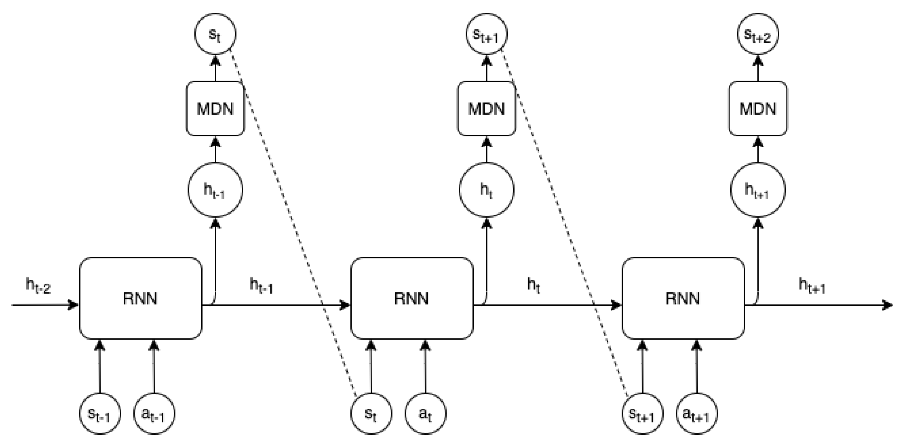
Ha & Schmidhuber [5] combined an incremental reward function and MDN-RNN state predictor to form a fully hallucinogenic world model. A controller receives current state s and takes an action a. These are concatenated together and the RNN outputs the parameters to the MDN. The world-model presents a sample taken from the MDN as the next state to agent, and the agent receives a reward if the state is not terminal. Figure 3 displays a visualization of how states are sampled over time in the world-model.
4. Design
It is straightforward to formulate bitrate streaming as a reinforcement learning problem. The state s is a vector , where is the throughput measurement, is the download time of the past chunk, is a vector of the m available sizes for the next chunk, is the size of the buffer, is the number of chunks that remain in the video, and is the selected bitrate of the previous chunk. The action a is the bitrate for the next chunk, and the reward r per time step is the contribution to the QoE function for time step t.
Many reinforcement learning algorithms are evaluated on collections of environments, such as the Arcade Learning Environment [28], RLLab [29], and OpenAI Gym [30]. These collections have a common interface and allow for researchers to easily experiment with novel algorithms. Moreover, they allow researchers to easily reproduce and evaluate the results. Until recently, there was no easy-to-use platform for experimenting and benchmarking problems in the computer systems domain. Many applications of reinforcement learning in computer systems require difficult configurations and the collection of traces in production systems. Park [7] is an attempt to lower the barrier to entry to machine learning research in the systems domain. The Park platform consists of 12 systems-centric environments, including both custom-built simulators and interfaces to real system environments. Park includes a bitrate streaming simulator that is based on the work in the Pensieve project [1]. This project leverages the Park simulators for ease of development and training. Algorithms to learn hallucinogenic world-models must successfully work on these simulated systems environment before they can be applied to larger, more complex systems, such as an entire data center. Park environments use an interface that is similar to OpenAI Gym; agents provide a valid action to the environment and receive a tuple containing the next state, the reward, and a boolean value marking the end of the episode. Multiple instances of the same Park environment can easily run concurrently, generating experience in parallel to speed up training and evaluation. We ported the Park environment to OpenAI Gym for easier installation and modification.
The default Park formulation uses the linear QoE, a linear combination of the bitrate and stall, for its quality function. The Park environment [7] supports a set of network traces, which contain a 3G/HSDPA mobile data set collected in Norway from commuters in transit [31], such as bus or train passengers. In order to avoid situations where bitrate selection is trivial (consistent high network throughput) or impossible (little to no service), the data set only contains traces where the average throughput is less than six Megabits per second (Mbps), and the minimum throughput is greater than 0.2 Mbps [1]. In addition, we have added a test set of extended traces from the Pensieve project to the Park environment.
4.1. World-Model Design
A fully hallucinogenic world-model requires an accurate state and reward predictor. It is straightforward to apply the MDN-RNN in order to predict state in the bitrate streaming environment. The state space for bitrate streaming is continuous, except for the number of chunks remaining in the video, which decreases by one until the episode ends. These experiments apply the MDN-RNN to the entire state space and assume that the remaining chunk predictions will contain a small rounding error.
The reward for bitrate streaming, QoE metrics, measures the quality of experience for the user across the episode, but it is computed at each step. This computation involves the previous state and action, and the current state and action. The action prior to each step, , is recorded in the state space at each step, . If an MDN-RNN is used to predict the next state given an action, then we can apply a function to compute the contribution to total QoE at each step, forming a fully hallucinogenic world-model. This method also has the advantage of allowing the QoE metric for performance to be substituted or changed as needed, without retraining the entire model. The reward function at each step is as follows:
Here, is the linear QoE parameter constant, (4.3 in the simulator), is the quality function on the current action, and is the rebuffering time, being computed from the previous buffer size and the time to download the current chunk. is the penalty term for bit rate change from the previous action. The world-model presents a state to the agent and the agent selects an action . The MDN-RNN samples the next state , and the world-model then computes the reward using the three inputs that it requires: . The world-model then passes the next state and computed reward to the controller. In the first step of the environment, the bitrate change penalty is set to 0, because the agent does not have a previous action.
Ha & Schmidhuber [5] used evolutionary algorithms to train their controller inside the world-model. Instead, we evaluate the ability of a model-free reinforcement algorithm to train inside the world-model.
4.2. Training Methodology
In theory, model-based algorithms can provide benefits to many systems problems; however, world-models have been seldom explored on non-robotic real-world problems. While metrics, such as mean-squared error or log-likelihood, give an indication of performance and they are used to train algorithms, these measures do not provide an intuitive measure of the robustness of a world-model. This work considers a world-model to be sufficiently accurate if a model-free algorithm that is trained inside the hallucinogenic world-model can achieve similar performance to the same model-free algorithm trained in the real environment. A model-free agent trained inside of the hallucinogenic world model will likely not reach the performance of the same agent trained in the real environment, due to imperfections of the world-model.
First, this project establishes baselines for maximum performance of a model-free agent trained directly in the Park environment. Furthermore, we establish baselines for two heuristics in the Park environment, RobustMPC and Buffer-Based. The world-model that is described above can be constructed using recorded observations, and a model-free agent can train entirely inside the learned world-model. We adjust the number of interactions with the environment to establish sample complexity baselines, and make comparisons with a state-of-the-art model-free algorithm, Rainbow [20].
5. Results and Discussion
5.1. Baselines
For bitrate streaming, this work uses an implementation of the Advantage Actor-Critic (A2C) algorithm from Stable-Baselines [32], a collection of implementations of common deep reinforcement learning agents. We obtained a copy of the Park authors’ bitrate streaming agent in order to validate the implemented agent used in this project. In correspondence, the authors noted that they added traces to the repository during publication and the results may have slight differences from the scores in the original paper. We performed a combination of grid search and refinement by hand on parameters for the value coefficient, starting entropy coefficient, entropy decay, and optimization algorithm. The entropy was decayed by the entropy rate every 264 steps and stops decaying once the entropy reaches zero. Figure 4 shows the training curve for the final model-free A2C agent trained entirely inside the Park environment.
Every 26,400 steps, the policy of the agent is evaluated for 10,000 actions. The solid blue line represents the average score at each evaluation step and the shaded portion highlights the standard deviation. The curve is jagged because the environment is stochastic, as evaluating the agent’s performance regularly with a high number of iterations impedes training. Through correspondence with the Park authors [7], we received their implementations for the buffer-based and RobustMPC heuristics. A random agent in the environment receives a score of . The provided Buffer-based and RobustMPC agents receive average scores of and over 1000 episodes, respectively.
5.2. Training in a Dream
A script collects traces from 10,000 episodes (five million total actions) episodes using a random agent to construct the world-model; all of the observations are normalized using min–max scaling from the bounds of the Park environment. This project uses a version of the MDN-RNN from Ha & Schmidhuber [5], which was modified to operate in the native bitrate streaming state space, without an autoencoder. The MDN-RNN is wrapped by a class to advance the state of the world-model, and compute the reward function, as described above. The wrapped world-model implements the OpenAI Gym interface; any controller compatible with this interface can train inside the hallucinogenic world-model. The following section contains the results from training both the MDN-RNN and training a controller inside the hallucinogenic world-model. Appendix A lists the parameters used in these experiments, and they were the same parameters used by Ha & Schmidhuber [5], unless otherwise noted. This project trained the MDN-RNNs using a smaller hidden state size to reduce possibilities of overfitting because the state space for bitrate streaming contains 12 values. Figure 5 shows the log-likelihood loss during training for an MDN-RNN with 64 hidden units and five Gaussians. We trained the established baseline agent inside of the fully hallucinogenic world-model. We performed a sweep on the temperature values in order to determine how increased difficulty in the world-model provides benefits for translation to the real environment. Table 1 contains the results of the parameter sweep. For each temperature, an A2C controller was entirely trained in the world-model with that temperature. Next, the controller was evaluated across 500 episodes in the dream environment, the actual environment, and a test environment. This procedure was repeated three times for each temperature value. The first three columns in Table 1 show the mean of the average score from each controller instance. At low temperatures, the agent can reach extremely high scores in the dream environment, but these scores do not translate to reality; an agent trained in a world-model with a temperature of 0.1 performs nearly four times worse than the performance of a random agent. As temperature increases, it becomes progressively more difficult for the agent to earn high scores in the dream environment. Noticeably, the agents that translate the best to the real environment (see temperature of 2.0) receive poor overall scores in the dream environment. The temperature hyperparameter can be tuned in order to find the optimal translation from the dream environment to the real environment. The average across runs in Table 1 shows that increasing the temperature increases scores in the real environment, and then decreases scores as the environment becomes too difficult to find a translatable policy. However, this behavior is not entirely consistent if one were to run a single sweep on temperatures. The rightmost column presented in Table 1 shows the average scores and standard deviations a single temperature sweep, tested in the actual environment. While a single sweep follows the general trend of increasing to a peak and then decreasing, the increase and subsequent decrease in scores are not always monotonic; the rightmost column presented in Table 1 highlights these discrepancies. In training, it is possible that an agent learns to exploit the world-model and fails to generalize to the real environment. The best A2C agent trained in the world-model received an average score of in the real environment, which is close, but does not beat the average score of for the same model-free agent. The world-model was trained with a total of five-million actions in the real environment, and the controller trained for ten-million actions inside of the world-model. The strictly model-free controller used ten-million actions in the real environment. While the model-free controller took more samples in the real environment for these experiments, these experiments do not show conclusive benefits concerning sample complexity.
5.3. Sample Complexity Bounds
5.3.1. Rainbow
We compare our results with the Rainbow algorithm to make fair comparisons on sample complexity [20]. Rainbow is considered to be state-of-the-art with regard to sample complexity, and was used recently in comparisons with a model-based algorithm, SimPLe [6]. We used a Rainbow implementation from the Dopamine package; further information is provided in Appendix B. We reduced the number of actions in the real environment to 1,000,000 (1M) for world-model construction and model-free training. For hyperparameter tuning, we used a combination of grid search and autotuning in order to optimize Rainbow. The grid search uses a nearly identical parameter space to [6]; these parameters are listed in Appendix B. We additionally completed 100 iterations of hyperparameter autotuning with the Optuna framework [33] to optimize the hyperparameter search space with the Tree-Structured Parzen Estimator method (TPE). TPE attempts to balance exploration versus exploitation by iteratively selecting hyperparameters with the largest expected improvement on model loss. For more information on TPE, this work refers readers to the original paper [34]. The best Rainbow model trained for 1M actions received an average score of in an evaluation of 500k actions.
5.3.2. World-Model Comparisons
We performed experiments training a model-free agent inside of a world-model trained from lower sample complexities: 1M and 500k actions. Table 2 and Table 3 show the results from these experiments. Training with lower sample complexities results in much less stability, but it still allows for performance that is nearly identical to the 5M-sample world-model. During some runs, an agent would learn policies that translate poorly into the real environment. Higher temperatures for the 1M-sample world-model presented in Table 2 result in greater world-model stability, and the performance was very similar between each repeated run.
The maximum average score of an agent trained in a world-model with only 500 k samples achieved a score of , which is higher than the average score of the best Rainbow agent that was trained with 1 M samples. There is no reason to believe that the Rainbow agent would improve performance with a lower sample complexity and, thus, we did not do further training for this sample regime.
5.4. Summary
Table 4 shows the compiled best scores for each agent at each sample regime. An agent trained entirely inside a world-model was able to achieve performance that was close to strictly model-free agent. Furthermore, an agent trained inside the world-model beats the scores of the provided heuristics. Additionally, these world-model agents learn more consistent policies that have lower variance when compared to the heuristics. The best world-model agents do consistently learn policies with lower variance than the model-free agents. Finally, the world-model agent was able to outperform a well-tuned Rainbow agent for lower sample complexities.
5.5. Future Work
Ha & Schmidhuber [5] passed the hidden state of the world-model to their evolution-based controller at each step. Further work may incorporate passing the hidden state of the world-model in order to a model-free controller.
Interpretability has become an issue across all areas of machine learning [35]; a human cannot explain decisions that are made by many machine learning algorithms. While not all systems require interpretability, it is important to have solutions that are easy to understand and debug. Heuristics are often easy to understand, and they can be easily engineered with specific safety properties [7]. When learning world-models on real systems, it may be essential to have a world-model detect uncertainty or unexplored parts of the state space and provide this information to the controller. In these cases, a controller that is trained in the world-model could fall back to a heuristic to avoid potentially damaging decisions.
6. Conclusions
This work does show that it can be straightforward to apply world-models to networking problems. The MDN-RNN world-model was able to capture the dynamics of the environment; however, these experiments required proper tuning of the temperature parameter in order to learn a policy that can translate into the real environment. Finding the optimal temperature hyperparameter for other environments may require sweeping several values, and these runs must be repeated. The optimal temperature was 70% higher than the optimal temperature that was used by Ha & Schmidhuber [5]. Furthermore, these experiments show a rapid decrease in performance after the sweep passes the optimal temperature. It may take careful tuning to find the optimal temperature in other environments. The experiments in this work demonstrate that world-models can successfully learn simulators from the recorded data. Furthermore, world-models can outperform model-free approaches in low sample regimes. World-models are a promising area of research that may provide benefits for many other problems in the networking and systems domains.
Author Contributions
This paper was produced from H.B.’s MPhil dissertation that was supervised by K.F. and E.Y.; H.B. prepared the draft; K.F. and E.Y. worked with H.B. to edit and review the paper. All authors have read and agreed to the published version of the manuscript.
Funding
This research was partially funded by the Alan Turing Institute.
Acknowledgments
This research was supported by the Alan Turing Institute.
Conflicts of Interest
The authors declare no conflict of interest.
Abbreviations
The following abbreviations are used in this manuscript:
| ALE | Arcade Learning Environment |
| A2C | Advantage Actor-Critic |
| A3C | Asynchronous Advantage Actor-Critic |
| GMM | Gaussian Mixture Model |
| LSTM | Long Short-Term Memory |
| MDN-RNN | Mixture Density Network - Recurrent Neural Network |
| MDP | Markov Decision Process |
| MPC | Model Predictive Control |
| MSE | Mean Squared Error |
| Mbps | Megabits per second |
| POMDP | Partially Observable Markov Decision Process |
| RL | Reinforcement Learning |
| RNN | Recurrent Neural Network |
| TPE | Tree-structured Parzen Estimator |
| QoE | Quality-of-Experience |
Appendix A. Bitrate Streaming MDN-RNN

Table A1.
Hyperparameters for bitrate streaming MDN-RNN.
| Num Steps | 4000 |
| Input Sequence Length | 12 |
| Output Sequence Length | 11 |
| Batch Size | 100 |
| RNN Hidden State Size | 0.00005 |
| Number of Gaussians | 5 |
| Learning Rate | 0.005 |
| Grad Clip | 1.0 |
| Use Dropout | False |
| Learning Rate Decay | 0 |
Appendix B. Rainbow Hyperparameter Search
To make fair model-free comparisons in low sample regimes, we compare our results with the Rainbow algorithm. We tuned hyperparameters for a Rainbow agent from the Dopamine package: https://github.com/google/dopamine/blob/master/dopamine/agents/rainbow/rainbow_agent.py.
Appendix B.1. Grid Search
60 iterations of grid search using the following hyperparameters. All runs used the default learning rate of 0.09.
- Target Update Period: {50, 100, 1000, 4000, 8000}
- Update Horizon: {1, 3}
- Update Period: {1, 4}
- Min Replay History: {500, 5000, 20,000}
Appendix B.2. Autotuner
100 Iterations of Tree-Structured Parzen Estimator operating in following parameter space. The learning rate is a continuous interval; all other parameters ranges are integer intervals.
- Learning Rate: (0.01, 0.15)
- Target Update Period: (50, 20,000)
- Update Horizon: (1, 8)
- Update Period: (1, 8)
- Min Replay History: (100, 40,000)
References
- Mao, H.; Netravali, R.; Alizadeh, M. Neural Adaptive Video Streaming with Pensieve. In Proceedings of the Conference of the ACM Special Interest Group on Data Communication, Los Angeles, CA, USA, 21–25 August 2017; pp. 197–210. [Google Scholar]
- Arulkumaran, K.; Deisenroth, M.P.; Brundage, M.; Bharath, A.A. A Brief Survey of Deep Reinforcement Learning. arXiv 2017, arXiv:1708.05866. [Google Scholar] [CrossRef] [Green Version]
- Kaelbling, L.P.; Littman, M.L.; Moore, A.W. Reinforcement Learning: A Survey. J. Artif. Intell. Res. 1996, 4, 237–285. [Google Scholar] [CrossRef] [Green Version]
- Schmidhuber, J. On Learning to Think: Algorithmic Information Theory for Novel Combinations of Reinforcement Learning Controllers and Recurrent Neural World Models. arXiv 2015, arXiv:1511.09249. [Google Scholar]
- Ha, D.; Schmidhuber, J. Recurrent World Models Facilitate Policy Evolution. In Advances in Neural Information Processing Systems 31; Curran Associates, Inc.: New York, NY, USA, 2018; pp. 2451–2463. Available online: https://worldmodels.github.io (accessed on 18 August 2020).
- Kaiser, L.; Babaeizadeh, M.; Milos, P.; Osinski, B.; Campbell, R.H.; Czechowski, K.; Erhan, D.; Finn, C.; Kozakowski, P.; Levine, S.; et al. Model-Based Reinforcement Learning for Atari. arXiv 2019, arXiv:1903.00374. [Google Scholar]
- Mao, H.; Negi, P.; Narayan, A.; Wang, H.; Yang, J.; Wang, H.; Marcus, R.; Shirkoohi, M.K.; He, S.; Nathan, V.; et al. Park: An Open Platform for Learning-Augmented Computer Systems. In Advances in Neural Information Processing Systems; Curran Associates Inc.: New York, NY, USA, 2019; pp. 2490–2502. [Google Scholar]
- Akamai. dash.js. Available online: https://github.com/Dash-Industry-Forum/dash.js/ (accessed on 18 August 2016).
- Huang, T.Y.; Handigol, N.; Heller, B.; McKeown, N.; Johari, R. Confused, Timid, and Unstable: Picking a Video Streaming Rate is Hard. In Proceedings of the 2012 Internet Measurement Conference, Boston, MA, USA, 14–16 November 2012; pp. 225–238. [Google Scholar]
- Bemporad, A.; Morari, M. Robust Model Predictive Control: A Survey. In Robustness in Identification and Control; Springer: Berlin/Heidelberg, Germany, 1999; pp. 207–226. [Google Scholar]
- Spiteri, K.; Urgaonkar, R.; Sitaraman, R.K. BOLA: Near-Optimal Bitrate Adaptation for Online Videos. In Proceedings of the IEEE INFOCOM 2016—The 35th Annual IEEE International Conference on Computer Communications, San Francisco, CA, USA, 10–15 April 2015; IEEE: Piscataway, NJ, USA, 2016; pp. 1–9. [Google Scholar]
- Huang, T.Y.; Johari, R.; McKeown, N.; Trunnell, M.; Watson, M. A Buffer-Based Approach to Rate Adaptation: Evidence from a Large Video Streaming Service. In Proceedings of the 2014 ACM Conference on SIGCOMM, Chicago, IL, USA, 17–22 August 2014; pp. 187–198. [Google Scholar]
- Chebotar, Y.; Hausman, K.; Zhang, M.; Sukhatme, G.; Schaal, S.; Levine, S. Combining Model-Based and Model-Free Updates for Trajectory-Centric Reinforcement Learning. In Proceedings of the 34th International Conference on Machine Learning, Sydney, Australia, 6–11 August 2017; Volume 70, pp. 703–711. [Google Scholar]
- Mnih, V.; Kavukcuoglu, K.; Silver, D.; Graves, A.; Antonoglou, I.; Wierstra, D.; Riedmiller, M. Playing Atari with Deep Reinforcement Learning. arXiv 2013, arXiv:1312.5602. [Google Scholar]
- Silver, D.; Huang, A.; Maddison, C.J.; Guez, A.; Sifre, L.; Van Den Driessche, G.; Schrittwieser, J.; Antonoglou, I.; Panneershelvam, V.; Lanctot, M.; et al. Mastering the game of Go with deep neural networks and tree search. Nature 2016, 529, 484. [Google Scholar] [CrossRef] [PubMed]
- Mnih, V.; Badia, A.P.; Mirza, M.; Graves, A.; Lillicrap, T.; Harley, T.; Silver, D.; Kavukcuoglu, K. Asynchronous Methods for Deep Reinforcement Learning. In Proceedings of the International Conference on Machine Learning, New York, NY, USA, 19–24 June 2016; pp. 1928–1937. [Google Scholar]
- Vinyals, O.; Ewalds, T.; Bartunov, S.; Georgiev, P.; Vezhnevets, A.S.; Yeo, M.; Makhzani, A.; Küttler, H.; Agapiou, J.; Schrittwieser, J.; et al. StarCraft II: A New Challenge for Reinforcement Learning. arXiv 2017, arXiv:1708.04782. [Google Scholar]
- Zhu, Y.; Mottaghi, R.; Kolve, E.; Lim, J.J.; Gupta, A.; Fei-Fei, L.; Farhadi, A. Target-driven Visual Navigation in Indoor Scenes using Deep Reinforcement Learning. In Proceedings of the 2017 IEEE International Conference on Robotics and Automation (ICRA), Singapore, 29 May–3 June 2017; IEEE: Piscataway, NJ, USA, 2017; pp. 3357–3364. [Google Scholar]
- Konda, V.R.; Tsitsiklis, J.N. Actor-Critic Algorithms. In Advances in Neural Information Processing Systems; MIT Press: Cambridge, MA, USA, 2000; pp. 1008–1014. [Google Scholar]
- Hessel, M.; Modayil, J.; Van Hasselt, H.; Schaul, T.; Ostrovski, G.; Dabney, W.; Horgan, D.; Piot, B.; Azar, M.; Silver, D. Rainbow: Combining Improvements in Deep Reinforcement Learning. In Proceedings of the Thirty-Second AAAI Conference on Artificial Intelligence, New Orleans, LA, USA, 2–7 February 2018. [Google Scholar]
- Dulac-Arnold, G.; Mankowitz, D.; Hester, T. Challenges of Real-World Reinforcement Learning. arXiv 2019, arXiv:1904.12901. [Google Scholar]
- Haj-Ali, A.; Ahmed, N.K.; Willke, T.; Gonzalez, J.; Asanovic, K.; Stoica, I. Deep Reinforcement Learning in System Optimization. arXiv 2019, arXiv:1908.01275. [Google Scholar]
- Buesing, L.; Weber, T.; Racaniere, S.; Eslami, S.; Rezende, D.; Reichert, D.P.; Viola, F.; Besse, F.; Gregor, K.; Hassabis, D.; et al. Learning and Querying Fast Generative Models for Reinforcement Learning. arXiv 2018, arXiv:1802.03006. [Google Scholar]
- Schmidhuber, J. Deep Learning in Neural Networks: An Overview. Neural Netw. 2015, 61, 85–117. [Google Scholar] [CrossRef] [PubMed] [Green Version]
- Hochreiter, S.; Schmidhuber, J. Long Short-Term Memory. Neural Comput. 1997, 9, 1735–1780. [Google Scholar] [CrossRef] [PubMed]
- Graves, A. Generating Sequences With Recurrent Neural Networks. arXiv 2013, arXiv:1308.0850. [Google Scholar]
- Bishop, C.M. Mixture Density Networks. 1994. Available online: http://publications.aston.ac.uk/id/eprint/373/ (accessed on 18 August 2020).
- Bellemare, M.G.; Naddaf, Y.; Veness, J.; Bowling, M. The Arcade Learning Environment: An Evaluation Platform for General Agents. J. Artif. Intell. Res. 2013, 47, 253–279. [Google Scholar] [CrossRef]
- Duan, Y.; Chen, X.; Houthooft, R.; Schulman, J.; Abbeel, P. Benchmarking Deep Reinforcement Learning for Continuous Control. In Proceedings of the International Conference on Machine Learning, New York, NY, USA, 19–24 June 2016; pp. 1329–1338. [Google Scholar]
- Brockman, G.; Cheung, V.; Pettersson, L.; Schneider, J.; Schulman, J.; Tang, J.; Zaremba, W. OpenAI Gym. arXiv 2016, arXiv:1606.01540. [Google Scholar]
- Riiser, H.; Vigmostad, P.; Griwodz, C.; Halvorsen, P. Commute Path Bandwidth Traces from 3G Networks: Analysis and Applications. In Proceedings of the 4th ACM Multimedia Systems Conference, Oslo, Norway, 28 February–1 March 2013; Association for Computing Machinery: New York, NY, USA, 2013; pp. 114–118. [Google Scholar]
- Hill, A.; Raffin, A.; Ernestus, M.; Gleave, A.; Kanervisto, A.; Traore, R.; Dhariwal, P.; Hesse, C.; Klimov, O.; Nichol, A.; et al. Stable Baselines. Available online: https://github.com/hill-a/stable-baselines. (accessed on 18 August 2018).
- Akiba, T.; Sano, S.; Yanase, T.; Ohta, T.; Koyama, M. Optuna: A Next-generation Hyperparameter Optimization Framework. In Proceedings of the 25rd ACM SIGKDD International Conference on Knowledge Discovery and Data Mining, Anchorage, AK, USA, 4–8 August 2019. [Google Scholar]
- Bergstra, J.S.; Bardenet, R.; Bengio, Y.; Kégl, B. Algorithms for Hyper-Parameter Optimization. In Advances in Neural Information Processing Systems; Curran Associates, Inc.: New York, NY, USA, 2011; pp. 2546–2554. [Google Scholar]
- Doshi-Velez, F.; Kim, B. Towards A Rigorous Science of Interpretable Machine Learning. arXiv 2017, arXiv:1702.08608. [Google Scholar]
Figure 1.
World-model pipeline. An agent trains inside the learned world-model and then is deployed back into the real environment.
Figure 1.
World-model pipeline. An agent trains inside the learned world-model and then is deployed back into the real environment.

Figure 2.
Recurrent Neural Networks allow for the network to retain information over time. Figure adapted from [26].
Figure 2.
Recurrent Neural Networks allow for the network to retain information over time. Figure adapted from [26].

Figure 3.
A state predicting Mixture Density Network with a Recurrent Neural Network (MDN-RNN). Figure adapted from [5].
Figure 3.
A state predicting Mixture Density Network with a Recurrent Neural Network (MDN-RNN). Figure adapted from [5].

Figure 4.
Training curve of an Actor-Critic (A2C) agent in the bitrate streaming Park environment.

Figure 5.
Training curve for an MDN-RNN with 64 units and five Gaussians.

Table 1.
World-model temperature parameter sweep. The rightmost column contains the mean episode score from a single parameter sweep for each corresponding temperature. While a single sweep follows the general trend of increasing to a peak and then decreasing, the increase and subsequent decrease in scores are not always monotonic; the rightmost column highlights these discrepancies. Note that the rightmost column contains the standard deviations of the episode scores for each agent, while the other columns contain the standard error of mean episode scores for three repeated runs.
| Temperature | Dream Score | Real Score | Test Score | Real (Single Sweep) |
|---|---|---|---|---|
| 0.1 | 2064.1 ± 1.7 | −22,010.7 ± 694.1 | −18,215.6 ± 632.6 | −22,010.75 ± 10,986.6 |
| 0.5 | 1036.9 ± 253.1 | −3801.2 ± 2115.6 | −2304.6 ± 1978.1 | −4965.1 ± 4222.8 |
| 0.75 | 649.5 ± 136.8 | −2461.0 ± 2165.7 | −1696.4 ± 1695.5 | −1159.8 ± 1754.6 |
| 1 | 726.1 ± 177.4 | −437.6 ± 776.2 | −13.4 ± 535.9 | −1317.7 ± 1781.3 |
| 1.1 | 770.0 ± 32.0 | 159.1 ± 189.7 | 370.5 ± 80.8 | 61.2 ± 810.6 |
| 1.2 | 569.7 ± 242.2 | 220.3 ± 92.9 | 339.4 ± 100.5 | 192.3 ± 365.1 |
| 1.3 | 594.0 ± 19.5 | 175.6 ± 101.2 | 367.1 ± 29.4 | 290.1 ± 367.2 |
| 1.4 | 406.8 ± 34.0 | 235.6 ± 120.4 | 370.6 ± 60.0 | 316.7 ± 274.6 |
| 1.5 | 305.5 ± 69.1 | 309.0 ± 64.5 | 449.3 ± 32.3 | 315.3 ± 349.0 |
| 1.75 | −177.7 ± 36.4 | 362.4 ± 30.2 | 444.7 ± 17.6 | 396.3 ± 279.9 |
| 2 | −952.0 ± 39.2 | 402.3 ± 8.8 | 476.2 ± 24.0 | 392.2 ± 193.5 |
| 2.25 | −5686.5 ± 5295.1 | −1595.8 ± 3052.8 | −1178.3 ± 2381.2 | 132.0 ± 46.1 |
| 2.5 | −7753.0 ± 5860.0 | −1585.1 ± 3039.7 | −1267.3 ± 2488.4 | 202.6 ± 383.1 |
| 3 | −17,087.6 ± 5885.9 | −3390.0 ± 3106.3 | −2570.8 ± 2434.8 | −5021.2 ± 4105.5 |
Table 2.
Temperature parameter sweep for a world-model trained from 1M recorded actions. The rightmost column contains the maximum mean episode score from an agent trained inside the world-model at the corresponding temperature. Note that the rightmost column contains the standard deviations of the episode scores for that agent, while the other columns contain the standard error of mean episode scores for three repeated runs.
| Temperature | Dream Score | Real Score | Test Score | Max Average Real Score |
|---|---|---|---|---|
| 1 | −3532.04 ± 2848.57 | −1525.94 ± 88.95 | 195.52 ± 100.36 | 282.45 ± 109.67 |
| 1.25 | −5666.19 ± 7003.71 | −4158.25 ± 2865.73 | −1205.58 ± 2329.62 | 132.80 ± 38.21 |
| 1.5 | −13,128.57 ± 10942.65 | −437.6 ± 6462.24 | −3375.84 ± 5514.53 | 320.92 ± 113.37 |
| 2 | −235.71 ± 13.72 | 369.18 ± 9.25 | 478.96 ± 3.26 | 378.79 ± 309.28 |
| 2.25 | −1628.17 ± 7.91 | 429.08 ± 11.65 | 557.84 ± 5.87 | 441.09 ± 316.88 |
Table 3.
Temperature parameter sweep for a world-model trained from 500,000 recorded actions. The data follow the same format as Table 2.
Table 3.
Temperature parameter sweep for a world-model trained from 500,000 recorded actions. The data follow the same format as Table 2.
| Temperature | Dream Score | Real Score | Test Score | Max Average Real Score |
|---|---|---|---|---|
| 0.75 | 550.04 ± 22.86 | −813.62 ± 764.66 | −403.87 ± 659.83 | 68.85 ± 826.89 |
| 1 | 453.31 ± 12.76 | 96.09 ± 50.03 | 382.93 ± 30.09 | 151.88 ± 826.91 |
| 1.25 | 291.33 ± 61.87 | −37.10 ± 132.88 | 247.92 ± 87.29 | 82.31 ± 648.22 |
| 1.5 | 158.27 ± 126.67 | 280.53 ± 182.38 | 428.88 ± 83.72 | 399.79 ± 245.12 |
Table 4.
Comparison between heuristics, model-free, and world-model agents for bitrate streaming.
| Num. Actions | Agent | Mean Episode Score | STDEV |
|---|---|---|---|
| - | Random Agent | −5729.3 | −4250.1 |
| - | Buffer-based Agent | 237.7 | 435.4 |
| - | RobustMPC Agent | 286.2 | 502.5 |
| 5 M | A2C Model-free Agent | 500.5 | 358.8 |
| 5 M | Best World-model Agent | 408.71 | 280.5 |
| 1 M | Best World-model Agent | 441.0 | 316.8 |
| 1 M | Best Rainbow Agent | 306.3 | 316.3 |
| 500 k | Best World-model Agent | 399.7 | 245.1 |
© 2020 by the authors. Licensee MDPI, Basel, Switzerland. This article is an open access article distributed under the terms and conditions of the Creative Commons Attribution (CC BY) license (http://creativecommons.org/licenses/by/4.0/).
Share and Cite
MDPI and ACS Style
Brown, H.; Fricke, K.; Yoneki, E. World-Models for Bitrate Streaming. Appl. Sci. 2020, 10, 6685. https://doi.org/10.3390/app10196685
AMA Style
Brown H, Fricke K, Yoneki E. World-Models for Bitrate Streaming. Applied Sciences. 2020; 10(19):6685. https://doi.org/10.3390/app10196685
Chicago/Turabian StyleBrown, Harrison, Kai Fricke, and Eiko Yoneki. 2020. "World-Models for Bitrate Streaming" Applied Sciences 10, no. 19: 6685. https://doi.org/10.3390/app10196685
Note that from the first issue of 2016, this journal uses article numbers instead of page numbers. See further details here.