Abstract
The aim of the paper is to describe a multicriteria model predictive control method for autonomous vehicles at non-signalized intersections. The centralized controller aims to describe control action for each autonomous vehicle to guarantee collision free passage. At the same time, performances are defined for the centralized Model Predictive Controller, namely the minimization of traveling time and energy consumption. Since these control goals are often conflicting, a scheduling variable is introduced to create a balance between them. Hence, the centralized controller can be tuned based on the importance of each control goal, which can be useful in urban environment where traffic densities may vary heavily depending on the period of the day. The effectiveness of the proposed centralized multicriteria controller is demonstrated through a complex simulation example in CarSim simulation environment using different tpye of autonomous vehicles.
1. Introduction
Significant part of the scientific research focuses on the challenges of control design of vehicles at non-signalized intersections. The basis of research is to determine the control design challenges related to the coordination of autonomous vehicles at intersection scenarios. In the US, there were more than 32 thousands fatal crashes on the roads in 2017 involving approximately 53 thousands vehicles and about 30 percentages of the human-driven vehicles participated in intersection accidents (see [1]). To decrease the number of fatal crashes related to human errors, it is attempted to analyze the use of autonomous vehicles in traffic systems. Traditionally the exact ordering at an intersection with traffic lights and signs is given by traffic rules followed by the driver of the vehicles. By the development of the automation in traffic systems, the coordination of autonomous vehicles at non-signalized intersection scenarios have become significant challenge of the control design.
A recent survey considering non-signalized intersection strategies is made by [2]. Multi-agent systems are developed for the control of non-signalized intersections and approached in several papers, see [3,4]. The proposed optimization algorithms are used to secure collision-free passage of vehicles through the intersection. The optimization problem for the control of autonomous vehicles crossing an intersection is reformulated as a convex program and solved by [5], while an optimal scheduling is proposed for the ordering problem as a Mixed-Integer Linear Program by [6].
For the determination of the crossing order of vehicles through the intersection Model Predictive Control (MPC) is used frequently to get an optimal solution by both centralized or decentralized controllers. An algorithm taking the expected entering time of vehicles into consideration is proposed to secure safe crossing of the intersection, see [7]. A decentralized MPC is used for the determination of time, while the negotiation between vehicles and the detection of the safety critical situations are guaranteed by vehicle-to-infrastructure (V2I) communication units. Two different decentralized MPC methods are presented to consider efficient fuel consumption, the requirement of comfort and to handle unexpected vehicle maneuvers during the passage through the intersection, see [8]. A MPC method is used for the assignment of priorities of automated vehicles to guarantee the optimal scheduling at the intersection by solving its control problem as a Mixed Integer Programming problem [9]. A bi-level, model predictive controller with coordination is presented by [10] to ensure the collision avoidance between automated vehicles at intersections. The optimization problem is solved by the use of a distributed Sequential Quadratic Programming method. In the control strategy optimal traveling speed is designed for each vehicle to secure safety constraints. An intersection crossing strategy by using a centralized controller is proposed by [11] formulating the control problem as a convex quadratic program, while a decentralized solution solving the local optimization problems of the sequence of the vehicles is developed by [12]. A centralized Optimal Control Problem (OPC) has been solved in a distributed fashion in [13] using a decomposition technique to create local OCPs with coupled constraints.
The contribution of the paper is a MPC-based multicriteria control method for autonomous vehicles considering both time duration of the intersection crossing and the total energy consumption of all vehicles. For safety and comfort reasons, constraints as speed limits, predefined minimum and maximum accelerations are built in the control strategy. As the purpose of the research is to determine the ordering of vehicles, the requirements of minimum traveling time and efficient energy consumption are incorporated in the control design, see also [10,14].
There are several benefits of the presented method compared to other strategies in the literature. Data-driven methods relying on machine learning techniques need to generate a great deal of possible scenarios defined by the autonomous vehicles position, speed, acceleration and turning intention. Moreover, little changes in the vehicles parameter space can result in very different solutions regarding the ordering and accelerations of the vehicle, which may lead to difficulties in the presence of sensor noises and uncertainties. Conventional MPC controls are superior in this sense, however, real-time implementation might be difficult due to the necessary computational power needed by the centralized controller. Presented method relies on a simplified optimization strategy, which is easy to implement and sufficiently fast for real-time applications.
The paper is organized as follows. The motivation of the research and the challenges in the control of autonomous vehicles at intersections are defined in Section 2. Section 3 shows the intersection scenario, describes the process of the MPC control design along with the constraints and performances defined. The proposed MPC intersection controller is validated in several simulation examples in Section 4. Finally, conclusions are drawn in Section 5.
2. Motivation
With the development of intelligent transport systems and the expansion of the applications of highly automated vehicles, transport scenarios are emerging that require the development of special methods in terms of control planning. The introduction of autonomous vehicles in traffic calls for a review of a number of traffic rules which, in addition to established habits and the ethical behavior of drivers, currently provide a solution in most traffic situations. However, for highly automated vehicles without a driver, these sets of rules are not applicable in all traffic scenarios. The control of autonomous vehicles at intersections is a significant challenge from the point of view of control planning. Currently, traffic lights, traffic signs and rules known to drivers ensure that vehicles pass through intersections without accident. When designing an intersection, engineers make a decision appropriate to the size of the traffic flow to use one of the above methods to reduce the number and magnitude of congestion or accident-prone situations. With the proliferation of autonomous vehicles, the spread of vehicle-to-vehicle (V2V) and vehicle-to-infrastructure (V2I) communication technologies and sensor fusion procedures, it is possible to trigger traffic rule-based management of intersections with intelligent intersection control. As an expected result of these research and development, in addition to increasing traffic safety, the development of congestion and the energy consumption of individual vehicles can also be reduced. In order to increase safety and comfort of the passengers, various conditions/limits (such as speed limits, acceleration limits) need to be incorporated into the control during design. A key task in planning the crossing is to determine the purpose of the intersection management. The primary goal is the safe passage of vehicles, which can be accompanied by performances such as minimizing transit time to avoid congestion and energy-optimal control to reduce fuel consumption and emissions. A balance between these often contradictory performances can be reached with multicriteria control procedures. The first step in planning the control of an automated intersection is to determine the passing order of the autonomous vehicles. Next, the control intervention for the implementation of the given order must be designed.
Problem Statement
The coordination of autonomous vehicles at an intersection can be more complex by
- the number of vehicles having different characteristics (e.g., related to danger or priority),
- different types of intersection,
- the predefined traffic rules considered in control design,
- the defined purpose of the control design of the vehicles like the minimization of time, energy losses and fuel consumption,
- the consideration of disturbances and uncertainties.
A non-signalized intersection scenario with several autonomous vehicles is proved to signify more complex situation in designing control for the crossing of the vehicles, see Figure 1. The safety condition of collision avoidance, the achievement of minimizing traveling time and the consideration of uncertainties of the measured data (e.g., distance of the vehicles from the origin of the intersection) affect to the design of multiple steps of control strategy. The proposed method considers most of the above-mentioned conditions increasing the complexity of the control of the intersection. The minimization of traveling time and energy of the vehicles passing through the intersection are in the focus of the coordination method.
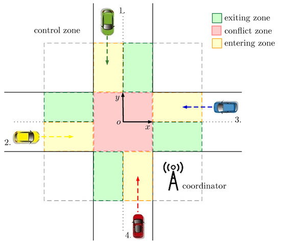
Figure 1.
Four-directional type intersection scenario.
Related to this field of control, several research studies maneuver and motion prediction of autonomous vehicles, see [15,16,17]. In connection with the driving intention of autonomous vehicles, detection of vehicle maneuvers using alert signals (e.g., brake lights, turn signals) are also of great importance, see [18,19]. A particular area of interest is the communication methods between the participants of the traffic and the infrastructures [20,21].
3. Model Predictive Intersection Control Design
3.1. Intersection Scenario
In the proposed intersection scenario vehicles can drive straight, turn left or right, therefore there is a probability of collision between vehicles tracking the same or different trajectories [22]. All features (e.g., velocity, driving intentions, position at the intersection) of autonomous vehicles are collected by a centralized controller transmitting measured data and control input for all participants of the traffic situation. The goal of the paper is to design an algorithm which guarantees collision-free passage of autonomous vehicles at intersections, while it minimizes the total traveling time or the energy consumed by the vehicles. Therefore, congestion at the intersection can be avoided and fuel consumption can be reduced while safety of the autonomous vehicles can be enhanced. In view of the intersection scenario, the goal of the centralized controller is to determine the ordering of autonomous vehicles as well as their accelerations with the consideration of total traveling time or energy consumption, and to guarantee collision-avoidance at the same time.
The proposed Model Predictive Control (MPC) algorithm is based on some pre-assumptions. A four-directional type intersection shown in Figure 1 is examined, which is separated into different sections.
Before reaching the control zone, each autonomous vehicle is self-controlled, supervised by its own cruise control system. When a vehicle enters the control zone, a velocity profile and a corresponding acceleration is calculated for it by the centralized intersection controller founded on the actual velocity and planned trajectory of the autonomous vehicle. The latter data along with the calculated accelerations are sent from the vehicle to the intersection manager and vice versa by communication methods. Although the iterative calculation detailed later takes into account up to four vehicles at a time, the calculation is repeated with reconfigured initial conditions in case a new vehicle enters the intersection. Note, that in case the new vehicle enters while the preceding vehicle is still ahead, it engages adaptive cruise control with a predefined spacing until the preceding vehicle leaves the intersection conflict zone. In this manner, the proposed algorithm can be enhanced to handle intersections having bigger traffic density. Moreover, the proposed algorithm can be augmented to consider more complex intersections as well.
3.2. Constraints for the Control Design
In the case of autonomous vehicles, speed limits must also be specified for safety reasons while crossing the intersection. The safe speed of autonomous vehicles is given by simplified vehicle dynamics: for left turn, for right turn and towards the straight line is calculated, where and are the radius of left and right turns at the intersection, g is the gravitational constant, is the coefficient of adhesion between the tire and the road, which is assumed to be described by estimation methods, see e.g., [23,24,25], is the speed limit. For a typical intersection with four directions and a lane width of 5 m, taking into account a tire-road adhesion factor of , the safe right-turn speed is km/h, the safe left-turn speed is km/h. Thus, as vehicles turning left follow a trajectory defined with a much bigger cornering radius then right turning vehicles taking a sharp turn, their maximally allowed velocities in the intersection is almost the double of right turning vehicles. Note, that vehicles heading straight do not need to meet any dynamic constraint, hence the speed limit is posed as maximally allowed velocity for them. Maximum and minimum accelerations are also set for the autonomous vehicles to ensure passenger comfort, maintain traction and prevent wheel slip. Here, the thresholds m/s and m/s are chosen based on [26].
For collision-avoidance, some other constraints must also be built in the control design. The base for the collision-free passage of the autonomous vehicles at the intersection is to set the condition that only one vehicle can be located in the conflict zone of the intersection at the same time. Consequently, the oncoming vehicle (independently of its predefined trajectory) can enter the conflict zone of the intersection only at the exit time of the previous vehicle.
3.3. Time-Optimal Intersection Control Design
One of the design goal is to minimize the crossing time of autonomous vehicles , therefore reduce the risk of a congestion emerging. This goal is achieved by ordering and accelerating vehicles to cross the intersection at the highest possible speed.
Hence, the control algorithm defines constant acceleration i∈ [1…n] for the vehicles entering the intersection, by which the maximum speeds on the given track available can be reached. First, the following computation is processed for vehicles entering the intersection:
where is the initial speed, is the initial distance of all vehicles from the intersection origin.
Corresponding to the specified conditions for acceleration, replaces the calculated accelerations when the thresholds are reached. In this case, the maximum entry speed in the conflict zone shall be changed as follows:
The essence of the coordination is to compare the travel time of autonomous vehicles at the intersection to prevent collisions during their crossing. In the process of minimizing travel time, conflict situations between autonomous vehicles are analyzed to control accelerations. Hence, altering the acceleration followed by the vehicles before entering the conflict zone of the intersection is integrated into the proposed algorithm. In case vehicles are in a conflict situation, the priority for passing through the intersection should be given to the vehicle with the least travel time. The rest of the vehicles reduce their acceleration to give priority for the first vehicle, then give priority to the vehicle leaving second in the same way. In the event of multiple vehicle conflicts, the algorithm takes into account the stopping of vehicles at the end of the entry zone and determines the waiting time for entering the conflict zone with a predetermined acceleration.
For the proposed method, the entry and exit times of each vehicle in the conflict zone must be calculated. At the intersection, the entry time of vehicles can be determined by solving the following second-order equation:
where i∈ [1…n] is the entrance time. Assuming constant accelerations in the entering zone, (3) is simplified as:
The time spent by the vehicles at the intersection shall be determined by assuming that the vehicle is traveling at a constant velocity when it gets to the conflict zone. Selecting in the conflict zone the time spent is given as follows:
where is the trajectory length corresponding with the turning intention.
If the autonomous vehicle has to stop to give priority to other vehicle (or vehicles), a waiting time is also computed. In this case, the value is set in order for the vehicle to stop in front of the conflict zone. The waiting time is defined as the difference between the final time of the previous vehicle and the entry time of the subject vehicle. After the conflict zone is free, i.e., , the autonomous vehicle enters the conflict zone with the predetermined acceleration , hence the travel time in the intersection is given as follows:
Finally, the travel time of each autonomous vehicles is the aggregate of the entry and exit times:
Founded on the on-board measurements sent by the autonomous vehicles to the intersection coordinator, the computation is evaluated as follows iteratively:
- First, the maximum vehicle speed i∈ [1…n] is defined for each vehicle, calculated based on the planned vehicle trajectory. Given the initial speed and the distance measured from the origin of the intersection, a constant acceleration of i∈ [1…n] is determined based on (1). In addition, if the maximum speed cannot be reached with predefined acceleration thresholds, the maximum speed can be modified by using (2).
- The time of entry into the conflict zone and the time of exit ∈ [1…n] is defined for all vehicles using (4) and (7). Potential conflicts are then determined by analyzing the time overlaps of each vehicle in the conflict zone. If no collision danger is detected, the autonomous vehicles use the previously calculated accelerations to cross the intersection.
- In the event of a conflict between two or more vehicles, the algorithm is evaluated as follows: vehicle with the minimum exit time i∈ [1…n] is given priority and does not change its formerly calculated acceleration. The algorithm follows by iteratively reducing the acceleration of other vehicles and recalculating their corresponding entry time using (4) until the entry time exceeds the exit time of the previous vehicle. This iterative calculation process is followed for every conflicting vehicle. The derived accelerations i∈ [1…n] are then used in the entry zone. In case the waiting time is greater than zero, the subject vehicle waits for the calculated time at the beginning of the conflict zone and then applies .
- Lastly, when a new vehicle enters the intersection, the algorithm follows the vehicle tracking mode until the previous vehicle leaves the intersection conflict zone. If this occurs, the above procedure shall be repeated with the new starting conditions for each vehicle in the intersection control zone.
3.4. Energy-Optimal Intersection Control Design
Another priority of the intersection management may be to minimize the total energy consumption of the autonomous vehicles. Here, the conditions listed in Section 3.2 along with collision avoidance and dynamic constraints must also be considered. However, when ordering vehicles and defining accelerations, energy optimality is a fundamental design element. Hence, the main difference from the time-optimizing algorithm is that the vehicles at the intersection are sorted not by travel time but by their kinetic energy i∈ [1…n]. This calculation assumes that each autonomous vehicle, in addition to its initial position and speed, sends information to the coordinator about its mass i∈ [1…n].
The iterative computation of the vehicle ordering by the intersection coordinator are as follows:
- The maximum speed i∈ [1…n] is calculated and an additional limit on the maximum speed is defined as . Here, the difference compared to the time-optimized algorithm is that only the negative acceleration can be assigned for vehicles.
- In the event of a conflict between two or more vehicles, the energy optimization algorithm is evaluated as follows: vehicle with the maximum kinetic energy i∈ [1…n] gets priority and does not change its acceleration. The algorithm then reduces the acceleration of the other vehicles in an iterative manner similarly as listed in the time-optimized solution, with the difference that the priority is always chosen based on kinetic energy.
3.5. Multicriteria Intersection Control Design
For the multicriteria control, the energy-optimal solution is tuned by selecting the maximal velocity for the autonomous vehicles in a different manner. The goal of the design, is to scale the velocity by which the autonomous vehicles arrive at the intersection. Hence, the result of the control algorithm will consider energy optimality in the ordering of the vehicles, but time optimality will also be considered due to the larger velocities the vehicles are allowed to enter the intersection conflict zone.
Remark: First, the maximal velocities are calculated, serving as the constraints for the vehicles. Next, a scheduling parameter i∈ [] is introduced, which scales the gap between the initial velocities and maximal velocities given by the speed limits as follows: . Thus, selecting stands for a solution where traveling time is also considered greatly, while choosing gives back the energy optimal solution, and between a mixed performance is given. The rest of the multicriteria algorithm is similar to that detailed in Section 3.4, with the difference of substituting in place of .
3.6. Operation of the MPC Controller
The operation of the intersection MPC control is shown in Figure 2. The coordinator of the intersection collects the position and velocity data , i∈ [1…n] of each autonomous vehicle entering the intersection at a discrete time step k using a sampling time , along with their turning intention . For the newly entered vehicle, a decision is made based on the position of the preceding vehicle, whether to add the vehicle to the MPC optimization process, or switch to adaptive cruise control mode. Note, that for the MPC optimization method the control performance can be set by the scheduling variable . At each discrete time step k, based on the predefined value the solution of the time-optimal, energy-optimal or multicriteria vehicle ordering is calculated based on the analytical method detailed in Section 3.3, Section 3.4 and Section 3.5 for a time horizon i∈ [1…n]. Note, that the time horizon depends on the vehicle states and the intersection geometry, and the optimization problem is solved in a single control problem for all vehicles. Moreover, newly entering vehicles only join the MPC optimization process when the preceding vehicle leaves the intersection, thus the optimization proceeds with maximum four vehicles at the same time. The solution of the optimization gives the control variables i∈ [1…n], which the autonomous vehicles in the intersection follow until the subsequent time step, where the optimization is repeated with the forward shifted horizon. Since the vehicle ordering and prescribed accelerations are recalculated at every time step for vehicles in the entering zone, a sampling time s is selected to avoid chattering of the control signals. Note that present MPC method is inherently robust against bounded initial errors in the measurement signals, since as the accuracy of the signals improve as the vehicles get closer to the intersection origin, the online recalculation of the MPC controller adjusts the vehicle order and control inputs to the punctual data.
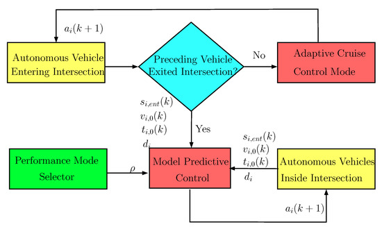
Figure 2.
Intersection control procedure.
3.7. Vehicle Control Model
The acceleration of the autonomous vehicles i∈ [1…n] calculated by the MPC controller is realized by applying a longitudinal force through the drive system. For this purpose, the following equation is implemented to derive the corresponding forces for the autonomous vehicles:
where i∈ [1…n] is the mass, is the control input, is the disturbance acting on the vehicle [27] including aerodynamic drag, rolling resistance and disturbance from the road slope.
The autonomous vehicles lateral trajectory tracking in the intersection is founded on the two-wheeled bicycle model, see [27,28]. The differential equations of the yaw motion is given as:
where v is the velocity, is the yaw angle, X and Y are the coordinates of the vehicle in a global coordinate system. Here, a simplified steering model is used with representing the steer angle, while L is the wheelbase of the vehicle and R is the radius of the road curvature.
Next, by using the relation , the state-space equations of the vehicle is given as:
Assuming small velocities and changes in the reference signals (; ), Equation (10) can be organized as follows:
where includes the error signals of the lateral position and yaw angle, is the steering input. The performance of the steering control is to minimize the error signals given in the state vector x. Hence, a Linear Quadratic (LQ) controller is applied using the cost function:
where Q and r are design parameters.
Solving the Ricatti equation the control gain K is derived, generating the steering input for the autonomous vehicles based on the measured error signals.
4. Simulation Results
4.1. Verification of the MPC Method
In order to analyze the effectiveness and time-optimality of the proposed MPC method, it has been compared to the result of a simulation-based optimization algorithm in CarSim environment. Note, that latter optimization technique can only be used for offline analysis and validation due to its big computational time.
For the sake of comparison, a four-directional double lane intersection has been chosen with four vehicles having initial conditions and turning intentions shown in Figure 3. As illustrated, Vehicle 1 and Vehicle are heading straight, while Vehicle 2 and Vehicle 4 are turning left with a 28 km/h speed constraint for entering the intersection.
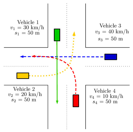
Figure 3.
Initial conditions for the simulation.
The simulation-based optimization algorithm is searching for the optimal acceleration values for each vehicles, by which they can safely pass the intersection without the danger of collision or skidding, while the total traveling time is minimized. The optimization algorithm running iteratively in MATLAB environment works as follows:
- Initialization: the upper and lower bounds for the acceleration values are calculated based on the intersection scenario. These values are used as bound constraints for the solution of the optimization. The starting point for the optimization is chosen to be zero acceleration for each vehicles.
- The constrained optimization algorithm runs the CarSim simulation with initial conditions and turning intentions depicted in Figure 3. The scheme of the CarSim multi-vehicle simulation is shown in Figure 4. Note, that the acceleration values for which the optimization algorithm is searching for are noted with ∈ [1…4], and are used as inputs for the simulated vehicles. The minimization function for the optimization algorithm is the total traveling time, which is measured by the CarSim simulation. The simulation ends when the last vehicle leaves the intersection conflict zone.
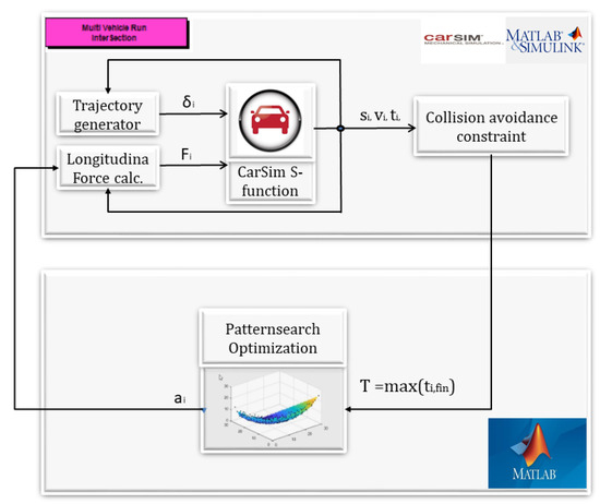 Figure 4. Optimization scheme in CarSim environment.
 - To guarantee collision free passing of the vehicles, the positions of each vehicles are measured, and a inter-vehicle distant constraint is built in the optimization procedure for avoiding them to get closer to each other more than 3 m. In this case, a large number is added to the traveling time measured in CarSim, thus the optimization algorithm discards the corresponding acceleration values.
- The constrained optimization runs the CarSim simulation iteratively until it founds acceleration values for the autonomous vehicles by which a local minimum for the traveling time is reached.
Next, the proposed time-optimal MPC intersection control has been evaluated with the same initial conditions depicted in Figure 3. The scheme of the real-time MPC control implemented in CarSim environment is depicted in Figure 5.
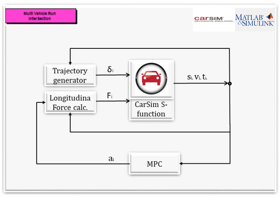
Figure 5.
Real-time MPC control in CarSim environment.
The result of the vehicle ordering and the traveling times spent in the intersection are shown in Figure 6.
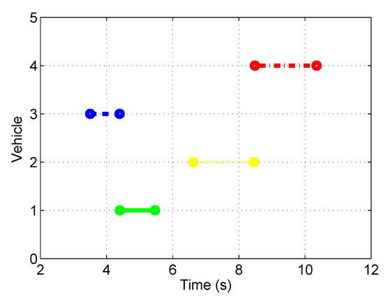
Figure 6.
Conflict zone travel times.
In the proposed time-optimal intersection control, Vehicle 3 crosses the intersection first, followed by Vehicle 1 and Vehicle 2, while Vehicle 4 finally leaves the intersection at s.
With the solution of the simulation-based optimization algorithm, the ordering of the vehicles are the same to that suggested by the proposed MPC controller. Here, the total traveling time of the vehicles are slightly smaller, with the last vehicle leaving the intersection at s.
Although the ordering of the vehicles are the same and the total traveling time is similar, the velocity profiles are different for the proposed MPC and the simulation-based optimization method, as depicted in Figure 7a,b. Note, that while the velocity of Vehicle 4 is similar for both cases, the other vehicles choose different acceleration values due to the nature of the underlying algorithm. With the solution of the simulation-based optimization, Vehicle 1, Vehicle 2 and Vehicle 3 selects very small acceleration values compared to the proposed MPC method. The latter method has the benefit mitigating the chance of a congestion to be formed in the intersection, as all of the entering vehicle tends to leave the intersection as soon as possible without holding the oncoming vehicles back.
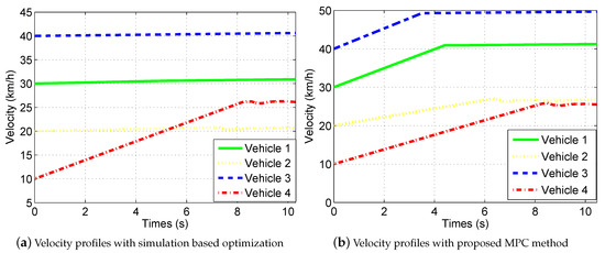
Figure 7.
Velocities of autonomous vehicles.
Hence, the comparison of the proposed MPC time-optimal method with the solution of the simulation-based constrained optimization showed that the total traveling time with the proposed method is very close to a global optimum given by the simulation-based optimization. Although in some cases, choosing different initial conditions a suboptimal solution might be given by the proposed MPC method, the online applicability due to small computational time is a very desirable feature.
4.2. Complex Simulation Example
The proposed method is also validated with a more complex example in CarSim environment. Here, four different type of autonomous vehicles arrive at the intersection, while a fifth vehicle also approaches the intersection entering zone and joins the proposed optimization as the preceding vehicle leaves the intersection. The initial positions and velocities of the autonomous vehicles along with their masses are shown in Figure 8. As illustrated, the intention of Vehicle 1 and Vehicle 3 is to continue heading straight, while Vehicle 2, Vehicle 4 and Vehicle 5 are intending to turn left.
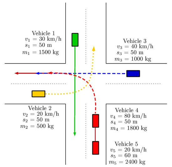
Figure 8.
Intersection scenario with five vehicles.
Simulations with the above detailed initial conditions were run with differently calibrated centralized controllers: first optimizing traveling time, secondly energy consumption.
The velocity and acceleration profiles of the vehicles running with the two different performance criteria are shown in Figure 9. In the case of the time optimal control law, Vehicle 4 crosses the intersection first, followed by Vehicle 3, Vehicle 1 and Vehicle 5, while Vehicle 2 finally leaves the intersection at s. As shown in Figure 9a the velocities of each vehicles increase at some point and Vehicle 1 and Vehicle 3 uses the maximal possible acceleration for a short period of time, see Figure 9b. Note, that Vehicle 4 having a big initial velocity decelerates heavily before entering the intersection conflict zone, and as all other vehicles, keeps an even velocity after entering.
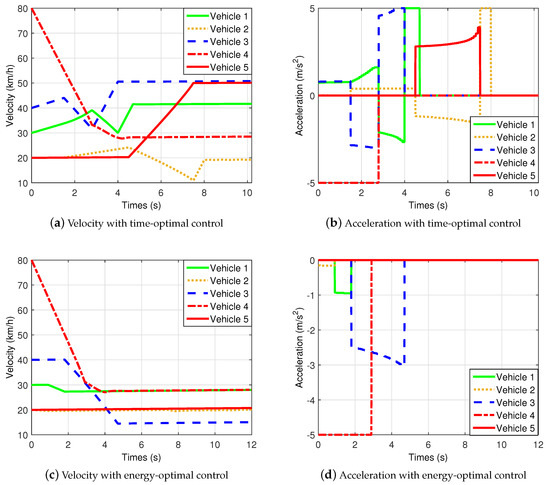
Figure 9.
Velocities and accelerations of autonomous vehicles.
On the other hand, with the energy optimal intersection control the vehicle ordering is changed significantly. Similarly to the time-optimal case, Vehicle 4 having big initial velocity and mass as well, leaves the intersection first. Next, Vehicle 1 also having bigger mass enters the intersection, followed by Vehicle 3 and Vehicle 2, while Vehicle 5 leaves the intersection finally at 12 s. Thus, in case of the energy optimal intersection control, the total traveling time of the vehicles increase by almost 2 s. Note, that in order to save energy, all vehicles only decelerate as shown in Figure 9d, decreasing their velocity before entering the conflict zone, see Figure 9c.
In Figure 10, the control energies (both driving and braking) of each vehicles are depicted along with the total control energy of all vehicles. It is well demonstrated, that the time-optimal solution shown in Figure 10a requires more than 2500 kJ of total control energy in contrast with the approximately 1700 kJ required by the energy-optimal centralized controller. Thus, for the given scenario, more than 800 kJ of total control energy can be saved in the intersection for the price of approximately 2 s in total traveling time.
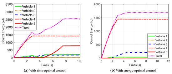
Figure 10.
Control energy of vehicles in the intersection.
Note, that above simulation scenarios where repeated with several different initial conditions. The proposed algorithm proved to be reliable, computationally efficient and fast enough for the simulation environment, hence it can be tested in real-time implementations.
5. Conclusions
The paper proposed a tunable intersection control algorithm for autonomous vehicles, with the aim to minimize both traveling time and energy consumption while guaranteeing collision free passage of the vehicles. For this purpose, a MPC has been designed with tunable performances. The proposed algorithm has been validated in CarSim environment by comparing its solution with a simulation-based optimization. Also, a complex example has been tested with a newly entering vehicle joining the optimization process. The results demonstrated the effectiveness of the proposed centralized controller.
Author Contributions
Conceptualization, methodology, software, A.M.; methodology, validation, Z.F.; supervision, P.G. All authors have read and agreed to the published version of the manuscript.
Funding
The research was supported by the Hungarian Government and co-financed by the European Social Fund, EFOP-3.6.3-VEKOP-16-2017-00001: Talent management in autonomous vehicle control technologies.
Conflicts of Interest
The authors declare no conflict of interest.
References
- National Highway Traffic Safety Administration. National Highway Traffic Safety Administration: Fatality Analysis Reporting System. 2019. Available online: https://www-fars.nhtsa.dot.gov/Vehicles/VehiclesLocation.aspx (accessed on 30 April 2020).
- Chen, L.; Englund, C. Cooperative Intersection Management: A Survey. IEEE Trans. Intell. Transp. Syst. 2016, 17, 570–586. [Google Scholar] [CrossRef]
- Dresner, K.; Stone, P. A Multiagent Approach to Autonomous Intersection Management. J. Artif. Intell. Res. (JAIR) 2008, 31, 591–656. [Google Scholar] [CrossRef]
- Zohdy, I.; Rakha, H. Optimizing driverless vehicles at intersections. In Proceedings of the 19th ITS World Congress, Vienna, Austria, 22–26 October 2012. [Google Scholar]
- Murgovski, N.; de Campos, G.R.; Sjöberg, J. Convex modeling of conflict resolution at traffic intersections. In Proceedings of the 2015 54th IEEE Conference on Decision and Control (CDC), Osaka, Japan, 15–18 December 2015; pp. 4708–4713. [Google Scholar]
- Fayazi, S.A.; Vahidi, A.; Luckow, A. Optimal scheduling of autonomous vehicle arrivals at intelligent intersections via MILP. In Proceedings of the 2017 American Control Conference (ACC), Seattle, WA, USA, 24–26 May 2017; pp. 4920–4925. [Google Scholar]
- Kneissl, M.; Molin, A.; Esen, H.; Hirche, S. A Feasible MPC-Based Negotiation Algorithm for Automated Intersection Crossing. In Proceedings of the 2018 European Control Conference (ECC), Limassol, Cyprus, 12–15 June 2018; pp. 1282–1288. [Google Scholar]
- Qian, X.; Gregoire, J.; de La Fortelle, A.; Moutarde, F. Decentralized model predictive control for smooth coordination of automated vehicles at intersection. In Proceedings of the 2015 European Control Conference (ECC), Linz, Austria, 15–17 July 2015; pp. 3452–3458. [Google Scholar]
- Yao, N.; Zhang, F. Resolving Contentions for Intelligent Traffic Intersections Using Optimal Priority Assignment and Model Predictive Control. In Proceedings of the 2018 IEEE Conference on Control Technology and Applications (CCTA), Copenhagen, Denmark, 21–24 August 2018; pp. 632–637. [Google Scholar]
- Hult, R.; Zanon, M.; Gros, S.; Falcone, P. Optimal Coordination of Automated Vehicles at Intersections: Theory and Experiments. IEEE Trans. Control. Syst. Technol. 2019, 27, 2510–2525. [Google Scholar] [CrossRef]
- Riegger, L.; Carlander, M.; Lidander, N.; Murgovski, N.; Sjöberg, J. Centralized MPC for autonomous intersection crossing. In Proceedings of the 2016 IEEE 19th International Conference on Intelligent Transportation Systems (ITSC), Rio de Janeiro, Brazil, 1–4 November 2016; pp. 1372–1377. [Google Scholar]
- De Campos, G.R.; Falcone, P.; Sjöberg, J. Autonomous cooperative driving: A velocity-based negotiation approach for intersection crossing. In Proceedings of the 16th International IEEE Conference on Intelligent Transportation Systems (ITSC 2013), The Hague, The Netherlands, 6–9 October 2013; pp. 1456–1461. [Google Scholar]
- Katriniok, A.; Kleibaum, P.; Josevski, M. Distributed Model Predictive Control for Intersection Automation Using a Parallelized Optimization Approach. IFAC-PapersOnLine 2017, 50, 5940–5946. [Google Scholar] [CrossRef]
- Gáspár, P.; Németh, B. Predictive Cruise Control for Road Vehicles Using Road and Traffic Information; Springer International Publishing: Berlin/Heidelberg, Germany, 2018. [Google Scholar]
- Lefevre, S.; Vasquez, D.; Laugier, C. A survey on motion prediction and risk assessment for intelligent vehicles. Robomech J. 2014, 1, 1–14. [Google Scholar] [CrossRef]
- Töro, O.; Bécsi, T.; Aradi, S.; Gáspár, P. Sensitivity and Performance Evaluation of Multiple-Model State Estimation Algorithms for Autonomous Vehicle Functions. J. Adv. Transp. 2019, 2019, 7496017. [Google Scholar] [CrossRef]
- Goodall, N.J. Real-Time Prediction of Vehicle Locations in a Connected Vehicle Environment; Final Report; Virginia Center for Transportation Innovation and Research: Charlottesville, VA, USA, 2013; pp. 1–55. [Google Scholar]
- Casares, M.; Almagambetov, A.; Velipasalar, S. A Robust Algorithm for the Detection of Vehicle Turn Signals and Brake Lights. In Proceedings of the 9th International IEEE Conference on Advanced Video and Signal-Based Surveillance (AVSS 2012), Beijing, China, 18–21 September 2012; pp. 386–391. [Google Scholar]
- Almagambetov, A.; Velipasalar, S.; Casares, M. Robust and Computationally Lightweight Autonomous Tracking of Vehicle Taillights and Signal Detection by Embedded Smart Cameras. IEEE Trans. Ind. Electron. 2015, 62, 3732–3741. [Google Scholar] [CrossRef]
- Shi, Y.; Pan, Y.; Zhang, Z.; Li, Y.; Xiao, Y. A 5G-V2X Based Collaborative Motion Planning for Autonomous Industrial Vehicles at Road Intersections. In Proceedings of the 2018 IEEE International Conference on Systems, Man, and Cybernetics (SMC), Miyazaki, Japan, 7–10 October 2018; pp. 3744–3748. [Google Scholar]
- Kokuti, A.; Hussein, A.; Marin, P.; de la Escalera, A.; Garcia, F. V2X communications architecture for off-road autonomous vehicles. In Proceedings of the 2017 IEEE International Conference on Vehicular Electronics and Safety (ICVES), Vienna, Austria, 27–28 June 2017; pp. 69–74. [Google Scholar]
- Shen, Z.; Mahmood, A.; Wang, Y.; Wang, L. Coordination of connected autonomous and human-operated vehicles at the intersection. In Proceedings of the 2019 IEEE/ASME International Conference on Advanced Intelligent Mechatronics (AIM), Hong Kong, China, 8–10 July 2019. [Google Scholar]
- Gustafsson, F. Slip-based tire-road friction estimation. Automatica 1997, 33, 1087–1099. [Google Scholar] [CrossRef]
- Li, K.; Misener, J.A.; Hedrick, K. On-board road condition monitoring system using slip-based tyre-road friction estimation and wheel speed signal analysis. Automatica 2007, 221, 129–146. [Google Scholar] [CrossRef]
- Alvarez, L.; Yi, J.; Horowitz, R.; Olmos, L. Dynamic Friction Model-Based Tire-Road Friction Estimation and Emergency Braking Control. J. Dyn. Syst. Meas. Control. 2005, 127, 22–32. [Google Scholar] [CrossRef]
- Bichiou, Y.; Rakha, H.A. Real-time optimal intersection control system for automated/cooperative vehicles. Int. J. Transp. Sci. Technol. 2019, 8, 1–12. [Google Scholar] [CrossRef]
- Rajamani, R. Vehicle Dynamics and Control; Springer: Berlin/Heidelberg, Germany, 2005. [Google Scholar]
- Kiencke, U.; Majjad, R.; Kramer, S. Modeling and performance analysis of a hybrid driver model. Control. Eng. Pract. 1999, 7, 985–991. [Google Scholar] [CrossRef]
Publisher’s Note: MDPI stays neutral with regard to jurisdictional claims in published maps and institutional affiliations. |
© 2020 by the authors. Licensee MDPI, Basel, Switzerland. This article is an open access article distributed under the terms and conditions of the Creative Commons Attribution (CC BY) license (http://creativecommons.org/licenses/by/4.0/).