GIS-Based Optimum Geospatial Characterization for Seismic Site Effect Assessment in an Inland Urban Area, South Korea


1
Earthquake Research Center, Korea Institute of Geoscience and Mineral Resources, Daejeon 34132, Korea
2
Department of Civil and Environmental Engineering, Seoul National University, Seoul 08826, Korea
*
Author to whom correspondence should be addressed.
Appl. Sci. 2020, 10(21), 7443; https://doi.org/10.3390/app10217443
Submission received: 18 September 2020
/
Revised: 14 October 2020
/
Accepted: 19 October 2020
/
Published: 23 October 2020
(This article belongs to the Special Issue Advances in Remote Sensing and GIS for Natural Hazards Assessment)
Abstract
:Soil and rock characteristics are primarily affected by geological, geotechnical, and terrain variation with spatial uncertainty. Earthquake-induced hazards are also strongly influenced by site-specific seismic site effects associated with subsurface strata and soil stiffness. For reliable mapping of soil and seismic zonation, qualification and normalization of spatial uncertainties is required; this can be achieved by interactive refinement of a geospatial database with remote sensing-based and geotechnical information. In this study, geotechnical spatial information and zonation were developed while verifying database integrity, spatial clustering, optimization of geospatial interpolation, and mapping site response characteristics. This framework was applied to Daejeon, South Korea, to consider spatially biased terrain, geological, and geotechnical properties in an inland urban area. For developing the spatially best-matched geometry with remote sensing data at high spatial resolution, the hybrid model blended with two outlier detection methods was proposed and applied for geotechnical datasets. A multiscale grid subdivided by hot spot-based clusters was generated using the optimized geospatial interpolation model. A principal component analysis-based unified zonation map identified vulnerable districts in the central old downtown area based on the integration of the optimized geoprocessing framework. Performance of the geospatial mapping and seismic zonation was discussed with digital elevation model, geological map.
1. Introduction
To evaluate regional geotechnical characteristics, multivariate information should be collected and normalized from the perspectives of geotechnical, spatial analysis, and remote sensing experts. Geospatial data are often limited or irregularly cover an area of interest. The available geospatial data are collected and analyzed based on geographic coordinates built into a geodatabase and processed through interpolation and zonal calculations based on geographic information system (GIS) techniques [1,2,3]. The collaborated approaches are feasible for combining the remote sensing based and subsurface in situ information in a map with high spatial resolution and spatial coincidence.
In civil engineering and related engineering practices, it is necessary to perform the geotechnical analyses [4]. Heterogeneity in geotechnical data may be governed by discontinuities in soil mass or geotechnical structures, and spatial or statistical biased properties [5]. It is well known that site characterization involves numerous inevitably variable characteristics and uncertainties when data is not directly assessed, but estimated using models and derived from other measured data [6,7,8]. Accordingly, the objectives of geotechnical spatial characterization are to determine soil and rock characteristics and to delineate subsurface stratigraphy for geotechnical engineering applications [9,10]. Thus, the successful implementation of geotechnical spatial characterization requires cooperation between geotechnical engineering and geoinformatics.
Methodological approaches for the establishment of geotechnical (or soil) property maps (e.g., engineering geo-layers or maps of in situ surveyed soil properties) with spatially scattered geospatial information provide good techniques for urban geology and development planning [11,12,13,14,15,16]. Recently, to demonstrate the multivariate dependencies of soil and rock in geotechnical big data, computational techniques are essential to support the analysis and interpretation of the increasing amounts of geoscientific data and information generated from data mining. The complexity of analyses in geotechnical behavior is due to the multivariable dependencies of soil and rock properties. Therefore, geotechnical mapping and subsurface sampling should have clearly defined spatial correlations that consider outliers and clustering of geotechnical information. Outlier detection is aimed at removing noise, finding possible and relevant information, and identifying optimized data that are distinctly different from others. Outliers in geotechnical spatial properties are difficult to define by statistical approaches, but it is possible to indicate the least predictable or relatively outlying data in the spatial domain using geostatistical modeling [17]. Hot spot analysis is a useful way to classify exactly where geotechnical and geological clustering zones are located [18].
Large metropolitan areas have high spatial variability in topography, geology, and subsurface characteristics as well as various urban developments. In such areas site assessments are largely based on the characteristics of soils and surface geology. Accordingly, it is necessary to comprehensively use surface index maps based on empirical correlations [19,20] and predict site response characteristics by processing sporadic soil survey data to grasp the site-specific zonal characteristics of highly reliable geo-layers and soil dynamic properties. In the event of an earthquake, near-surface ground motion may have very different intensity and frequency components depending on site effects. Therefore, site-specific response prediction methods provide rapid seismic response through regional seismic disaster prediction, including the seismic susceptibility of structures without numerical site response analysis, and seismic design through site-specific ground motion prediction. They can also be used directly for seismic performance evaluation.
A previously developed method of geospatial evaluation of borehole datasets based advanced geotechnical information system (GTIS) framework has been applied to several metropolitan areas (Seoul, Incheon, and Busan) in South Korea [21,22,23]. The proposed framework provided multivariate statistical clustering and geostatistical optimization for spatial visualization of site response parameters. However, the confined spatial analysis tools were only applied to the development of multivariate seismic zonation without comprehensive consideration of geotechnical and geostatistical correlations. Thus, methods are needed that consider geospatial variance in the unification and assessment of priorities that influence seismic site effect parameters, which will assist in better decision making. This study proposes a sophisticated framework by stepwise geospatial and geotechnical analysis models, which include geotechnical database (DB) optimization, hot spot analysis, geostatistical interpolation, and the generation of site response parameters. The mapping of the associated site response parameters will provide basic guidelines for understanding earthquake hazard scenario in any region.
2. Interactive Geospatial Database and Data
To investigate site-specific surface and subsurface conditions in Daejeon city, a comprehensive repository of data, such as borehole logs, a digital elevation model (DEM), an administrative division map, and geological maps, was collated based on existing ground survey data. (Figure 1). The study area including administrative division is within 35.0 km west to east and 44.0 km north to south. The surficial thematic coverages having high spatial resolution in Daejeon city are especially collected. The study area was defined as the area covered by the Daejeon administrative division map (Figure 1a), which was obtained from the National Geographic Information Institute in Korea. The administrative district was specified along with spatial coordinates. The DEM of the study area (Figure 1b) consisted of a grid with a 5 m × 5 m mesh size, maximum elevation of approximately 900 m, and an average standard deviation of 5.8 m. A slope map (Figure 1c) was extracted from the DEM, and the maximum slope was approximately 80°. A geological map of the study area (boundaries and faults; Figure 1d) was generated from the 1:50,000 scale geological map data that was obtained from the geological information management system at the Korea Institute of Geoscience and Mineral Resources. The average elevation and slope in building zone (Figure 1e), where Quaternary alluvium was mainly distributed, were 15 m and 6°, respectively. The drainage basin along Gapcheon stream are covered in the central region in building zone. The susceptible region against seismic site effect was mainly reported at the basin or basin-edge regions [19].
The main bedrock in the Daejeon area are metamorphic sedimentary and igneous rocks that have undergone low–medium grade metamorphism, and granitic and mafic intrusions [24]. The urbanized river basin of Daejeon city comprises Miocene (~20 mya) non-marine to deep marine sedimentary strata [25]. Soil development is mainly a result of fluvial landform processes. Zones with thick soils and deep bedrock are susceptible to ground motion amplification due to site effects during earthquakes. The DEM and geological map was used to review the performance of stepwise geoprocessing procedures and combine with the geotechnical characteristic.
The borehole log datasets (Figure 1f) were specifically designed as a geotechnical DB and are essential for characterization of seismic site effects. They were obtained from the Geo-Info system of the Korea Institute of Civil Engineering and Building Technology, and contained 3304 drilling survey datasets from a total of 153 projects. Engineering geo-layers were classified as fill layer (FL), alluvial soil (AS), weathered soil (WS), weathered rock (WS), and soft rock (SR), and their thicknesses and depths were extracted. The standard penetration test (SPT)-N (blow counts) value from each survey site was corrected by considering an N-value 60% of the energy efficiency (ER) [29]. Moreover, was linearly extrapolated based on 50 N-values, and the maximum was regulated under 300. When an N-value is 150 or above, reliability of the associated geotechnical characteristic value cannot be guaranteed. In this study, the extrapolated () was extracted as an average for each geo-layer. The seismic response parameter was determined using an empirical correlation [30], with based on the shear wave velocity (VS) within each geo-layer (FL, AS, WS, WR, and SR). If N value is not recorded above engineering bedrock (SR or normal rock), the representative vs. values were determined to be 190 m/s for FL, 280 m/s for AS, 350 m/s for WS, 650 m/s for WR, and 1300 m/s for bedrock [22].
Datasets in the geospatial DB were overlaid on a regular 100-m-mesh layer and the DEM that had been resampled to a 100 × 100 m mesh size. An intergraded mesh spatially joined by the geospatial DB provided geospatial information about the terrain, geology, and subsurface, and assigned a value to every vertex in the spatial structure. Thus, the DB could be analyzed and visualized by assigning a preprocessing phase (Figure 1) to the geotechnical characteristic values and interpolating data between vertices according to the mesh topology. Interactive DBs are playing an important role in the design, calibration, comparison, and optimization of proposed geospatial and geotechnical models [30]. In particular, units of sub-grouped meshes in two-dimensional domains are becoming the representative zonal statistics for detailed regional assessments.
3. Geospatial Informatics of the Geotechnical Database
Geotechnical spatial information containing errors and uncertainties should be verified and refined prior to determining geotechnical characteristics and design values. In particular, borehole log datasets, spatially projected as points in a two-dimensional domain can provide validation data regarding engineering strata and soil stiffness. To generate reliable site response parameters and an associated site classification, a preprocessing phase was proposed based on geoinformatics. The major tasks identified (Figure 2) included four sub-sequences: (1) optimization of the geotechnical DB, (2) hot spot analysis, (3) geospatial interpolation, and (4) generation of site response parameters. These can be implemented using a sophisticated computerized framework.
First, quality assurance criteria were used to screen borehole log data for incorrect properties. Outliers introduced by an investigation and data digitization were initially detected using a geostatistical approach. Borehole log data were excluded from the next step. Hot spot analysis is a spatial analysis and mapping technique that identifies clusters of spatial phenomena [31]. There are different methods for analyzing spatial patterns and detecting hot spots, including spatial autocorrelation and cluster analysis: (1) Kernel density estimation, (2) local Moran’s I, and (3) Getis-Ord Gi* statistics [32]. These were used to sub-group the optimized geotechnical DB focusing on hot spot clusters with statistical and spatial correlated values for the site response parameters.
To build zonal information with geotechnical characteristic values an appropriate spatial interpolation technique is essential. Among the various conventional methods, inverse distance weighting (IDW), simple kriging (SK), ordinary kriging (OK), and empirical Bayesian kriging (EBK) were used. The optimum method with the highest prediction accuracy was selected by comparing the prediction residuals from its cost function. Sequentially, the geotechnical database was optimized and then spatially grouped, followed by the building a grid database. Based on preprocessing results, each seismic zonation that correlated with site response parameters was mapped. Finally, the zonation maps were unified using principal component analysis (PCA) of the site class.
The uncertainty assessment of detected outliers in geotechnical characteristic value was verified with terrain and geological characteristics. The site condition of the sub-group in geotechnical DB was also reviewed according to surficial variation, and the geospatial interpolation and site zonation were assessed and visualized for incorporation of remote sensing data into geotechnical grid by building grid database with high spatial resolution.
3.1. Optimization of the Geotechnical Database
In geotechnical engineering practice, various borehole layout schemes are used to design a one-dimensional geo-layer profile and its characteristic coefficient. Since borehole log information is interspersed in time and place, there are inherent instabilities in the integrity of geotechnical DBs. These arise from differences in the purposes of the projects, ideas and techniques of the investigators and analyzers, and equipment performance. When experiments are translated into soil design properties with empirical or theoretical models, transformation uncertainty is added. Such uncertainties make geotechnical designs less reliable [33]. In measurements with appropriate statistical methods applied, it is important to minimize or eliminate “errors”. Thus, for reliable post-processing, the blended definition of the attribute or biased value from a borehole log should be checked for abnormalities in the geotechnical DB. Accordingly, quality assurance procedures were established first (Figure 3) to verify and exclude errors based on the standardized schemes used to develop the geotechnical DB.
Coordinates, engineering geo-layers, and SPT results are required to evaluate seismic site effects. The engineering geo-layers consist of four types: FL, AS, WS, WR, and bedrock (rock below soft rock). In a partial borehole log or when unreliable measurements are excluded, missing values are introduced. If the composition and thickness of a geo-layer or other required information is missing, it will be deleted. Input errors such as typographic errors in the geo-layer definition, thickness (e.g., 2505 m), and SPT-N (e.g., 12.5) were corrected manually. In 2007, the Korean government officially chose to follow the global geodetic reference system (ITRF and GRS80). The coordinates of boreholes investigated before 2007 were transformed. The standard transformation protocol adopted by the National Geographical Information Institute, South Korea, was applied [34].
To determine the geo-layer boundary and the correlated index property of soil, the geo-layer was classified according to the Unified Soil Classification System (USCS) [35]. The USCS classifies the geomaterial composition, measured in core samples from a borehole. In the same borehole, if the geomaterial did not match USCS criteria it was excluded from the geotechnical DB. The ground elevation of the borehole log was also shifted to match the elevation of the DEM (Figure 1b) at the borehole location.
Even though screening and calibration of errors was carried out, the inherent soil variability induced by geologic processes and uncertainty is introduced in transformations into empirical or theoretical models [17]. Usually, irregular measurements are numerically far away (usually in 10% confidence interval) from the remainder of the results, or may vary substantially from other nearby observations [17,36,37]. The spatial uncertainty and bias of geotechnical parametric values undermine the prediction accuracy of geospatial interpolation. Accordingly, we introduced geotechnical outliers that are numerically distant from the rest of the data or may deviate significantly from nearby observations [7,17,38].
In this study, a hybrid model blended with a cross-validation-based method [17] and Anselin Local Moran’s I statistic-based method [39] was proposed and applied to the screened bedrock depth in the geotechnical DB of Daejeon city (Figure 4).
Engineering bedrock was defined as rock strata below soft rock. Cross-validation is a consistency test for variograms or kriging models [40,41,42,43]. Calculated properties were tailored for the measurement of local reliability by a sequential blind test. Almost 10% (5% too high and 5% too low) of the prediction residuals was calculated for the outlier threshold with reasonably least accurate data points, by comparing the measured and estimated values by cross-validation. Most outliers that had high cross-validation residuals were spatially linear, and distributed along roads and railroads.
The local Moran’s I index is the most popular hot spot and spatial clustering method [39,44]. The index analyses each location and allows hot spots to be distinguished based on comparisons with neighboring samples. It shows the similarity of nearby features through the I value (–1 to 1) but does not indicate if the clustering is for high or low values. A positive I value indicates that the data is surrounded by similar values, either high or low. A high negative local I value (H-L or L-H in Figure 4b) indicates that the studied position is a spatial outlier. Spatial outliers are distinctly different from the values of their surroundings [45]. Spatial outliers include high-to-low and low-to-high outliers. Spatially intersected outliers (300 borehole logs) that were detected by both methods, were removed from the borehole log datasets (3304 borehole logs). At location of the outlier, elevation, and slope (Figure 1a,b) are mostly over 50 m 20° in the mountain and hill areas, where Jurassic granite was distributed in geological map (Figure 1d). Since 80% or more borehole datasets are densely distributed in basin area, sparse and few datasets having low spatial autocorrelation were usually selected as outlier. Approximately 3000 borehole log datasets were used for analysis.
3.2. Hot Spot Analysis of the Geotechnical Database
In contrast to the predicted number of occurrences within a random distribution, a hot spot may be defined as a region with a greater event concentration. The discovery of hot spots has been developed by the study of spatial points or spatial configurations [33]. The density of points within a certain region is compared to a completely random model in geospatial pattern analysis. In addition to density measurements and the grouping of correlated datasets, hot spot techniques often calculate the extent of the association between point events [46]. Spatial clustering methods such as kernel density estimation (KDE), local Moran’s I, or Getis-Ord Gi* statistics are therefore required to avoid the fragmentation of hot spots. In this study, these hot spot analyses were applied to the geo-layer thickness and average (Figure 5).
The KDE approach is a non-parametric procedure that uses a technique to estimate spatial density using a kernel function to fit a smoothly tapered surface to each point [47,48]. The kernel density represents a smooth and continuous surface map because interpolation generates a continuous discrete pattern [49]. The kernel calculator can be defined for a particular set of observations from an unknown probability density function:
where is the value of the variable at location i, n signifies the total number of locations, h is the smoothing parameter or bandwidth, K is the kernel, and is the estimator of the probability density function [50]. After KDE analyses of the Daejeon dataset, each geo-layer shows localized densities that are focused on central and northern parts of the urban region of Daejeon city (Figure 5). In the case of average for each geo-layer, the density trends were more remarkable in the order AS > WR > FL > WS. The resemblance between the local density of a geo-layer’s thickness and average suggests that the higher density areas of the geo-layer have the higher soil stiffness. KDE is only useful for aggregating spatially consistent grid data and is not suited to fragmented, location-based data [51].
Local Moran’s I can also be used to classify hot spots using Getis-Ord Gi* statistics, but in practice, Getis-Ord Gi* statistics (or Gi* statistics) have been shown to be superior. High concentrations and spatial outliers of geo-layer thickness and average (described by Anselin Local Moran’s I statistic-based outlier analysis) are samples surrounded by normal or low-value samples [37,44]. Local Moran’s I is more convenient for locating high or low values and outlier statistically relevant clusters. It is defined as follows:
where is the average value of x with sample number n, is the variance of variable x, and is a weight that can be defined as the inverse of the distance between locations i and j. The weight can be calculated using the distance bands. If the distance from neighbor j to feature i is within a distance band, , otherwise [51]. Areas with high Moran’s I values are higher than average. Only a single estimate of Moran’s I is given in the global version of Moran’s I for an overall area. This statistical approach underlines the level of events of each neighborhood characteristic and is thus less susceptible to spatial weighing characteristics than the aggregate level of events for the entire neighborhood [52]. In Daejeon city, because most values in the borehole dataset have similar distance bands, the spatial deviations of Moran’s I are not significant for every geo-layer.
The kernel density calculates Getis-Ord statistics for the thickness and average of each geo-layer for local clusters to identify seismic site effect parameters [53]. The Getis-Ord Gi* of the target geostatistical characteristic value in each geo-layer is analyzed to help identify where hotspots (high-value clusters) and cold spots (low-value clusters) in an area are located [44,54].
where is the Z-score of patch i, and is the attribute value for patch j. The Getis-Ord statistics were calculated using geostatistical characteristic values for each geo-layer, defined as the ratio of total values to the global total. The spatial clusters, based on confidence distributions, were classified into three “cold spot” (90%, 95%, and 99% confidence intervals), three “hot spot” (90%, 95%, and 99% confidence intervals), and one “not significant” sites. For soil deposits (FL, AS, and WS), the hot spot areas of the geo-layer thickness data were concentrated in the central urban region (elevation < 10 m; slope < 12°; mainly quaternary deposits in Figure 1). The northern area was categorized as a hot spot after applying Getis-Ord statistics to WS thickness.
In general, there is a strong positive relationship between the geo-layer thicknesses according to the KDE and Getis-Ord Gi* statistic methods. Land surface characteristics in primarily the central and partially the northern urban areas were categorized as the highest density area and as hot spot zones, where spatial correlations between thick soil deposits and high soil stiffness are strong. Even though the DEM and geological map are available, interpolations were restricted to borehole datasets from within the Daejeon administrative division for soil mapping at high spatial resolution, by using sub-group in borehole datasets having high correlation and density. The multi-scale grid zonation for geospatial interpolation was subdivided into two regions: a 20 m × 20 m grid for the central zone (elevation < 10 m; slope < 12°; area of interest with a hot spot and high K) and 50 m × 50 m grid for the others. According to Sun and Kim [23], response parameters were estimated based on the optimized grid at 20 and 50 m intervals. Borehole datasets were also clustered according to the two multi-grid zones. The geospatial interpolation results are resampled into the multi-scale grid.
3.3. Geospatial Interpolation
To predict reliable zonal geotechnical characteristics for the study area, the best-fitting geospatial interpolation model with the lowest prediction residuals was selected. Kim et al. [3,55] suggested an optimization procedure for geostatistical analysis of soil properties. A step-by-step adaptive optimization technique that used a GIS platform and geostatistical methods [56]. Cross-validation verification tests were applied using the four interpolation methods IDW, SK, OK, and EBK. The grid-based interpolation and zonation with DEM was assessed to build the reliable surficial geometry assigned with engineering geo-layer thickness and average (Figure 6 and Figure 7).
The effect of sample size according to distance is arbitrarily weighted by IDW, while kriging requires a variogram that models the spatial autocorrelation of data to give weightings. In IDW, unknown areas are specified only by known z-values and distance weights [57]. Kriging is a representative geostatistical interpolation method that quantifies and analyzes distance by variogram, and the estimators are variants as follows:
where is a known stationary mean, presumed to be constant across the entire domain and is the average of the data measured [58], is the kriging weight, n is the number of samples, and is the mean of samples. SK is modified based on Equation (4) as follows:
Therefore, SK is often referred to as medium kriging as residuals from the reference value [56]. The OK method is similar to SK, and the only difference is that OK estimates the value of the attribute using Equations (5) and (4) by replacing μ with a local mean, which is the mean of samples within a search window. The variance in ordinary kriging estimates is the sample variance if all the survey sites are measured, and the interpolation variance in the test position is equal to zero [59]. By considering the error in the variogram model calculation, EBK varies from SK and OK. The EBK method includes two geostatistical models: random intrinsic function kriging and a linear mixed model [60,61]. It simulates variograms for different sub-populations of the initial data.
Figure 6 and Figure 7 show geospatial maps of geo-layer thickness and average for each of the four interpolation methods. Figure 8 also presents the relationship between measured based on the interpolated multiscale grid (53791 cells).
Even though there were regional variations in each of the interpolation methods, they all showed soil layers in the vicinity of major urban riversides to be relatively thick where major infrastructure and residential areas were concentrated. In addition, the weathered layers (WS and WR) were relatively thicker in plains and downtown areas. Thus, the soil layer, which is a prominent factor in seismic site effects, is thickly distributed in areas where the population and industry are close, and the risk of damage due to an earthquake is higher. The geological map also showed relatively thick soil centered in areas where the bedrock is overlain by Quaternary sediments. The soil deposits in the river basin is thicker (up to about 40 m), and bedrock depth is deeper (up to about 70 m) than in mountain regions. In the case of average , the southern and northeastern regions have considerably higher (>250), where mountains and hills are located. These regions were also classified as cold spots and have lower K.
Root mean square errors (RMSEs) based on cross-validation were calculated for the best-fitting model. The sequential value at each sampling point was calculated by computing an experimental variogram and a kriging model, after exclusion of the measured target values at a given point. Differences between the predicted and measured values (geo-layer thickness and average ) were compared, and prediction residuals were computed for each borehole dataset (Figure 8). Geo-layers with shallower depths (i.e., closer to the surface) and lower showed greater fluctuations in the prediction residuals. This is because values in shallower geo-layers with low soil stiffness are concentrated. For the interpolations of thickness, the average residuals ranged between −5 and −5. On the contrary, the average residuals of average ranged between −100 and −100.
The ratio between the measured and predicted values was derived based on linear regression. The IDW technique showed better predictions, with an approximate ratio of 1:1 with measurements. Among the kriging methods, SK estimated similar values with measurements compared to OK and EBK. The predictions became more reliable as RMSE approached zero in the following order: AS, FL, WS, and WR. Most boreholes were drilled on plains with lower morphologic variability (deviation of elevation < 5 m; deviation of slope < 1°), where soil deposits were accumulated. Accordingly, there were numerous variants of AS and FL, and where sampling is quite regular, and spatial correlations are strong the prediction reliability was improved. This study focuses on demonstrating that site-specific geometry developed using IDW is a powerful predictor of the locations of thin soil deposits with low stiffness.
Thus, stochastic correlations between the upper boundary depth of each geo-layer and the average were estimated based on the grouped mean on unit depth assigned in the interpolated multiscale grid (53,791 cells) (Figure 9).
For FL, the deeper the depth, the greater the . For AS, increased to approximately 7 m depth, after which it decreased. The depth variation of for the weathered layer was not significant. When only a subsurface stratum is determined, can be predicted using the regression equations for each geo-layer type and thickness.
4. Multilayered Local Zonation of Seismic Site Effects
4.1. Site Response Parameters and Classification
Spatial zoning of site response parameters in Daejeon city was conducted based on geospatial characterization procedures. Using the optimized DB to screen and exclude outliers, a multiscale grid information was generated using IDW interpolation for each geo-layer thickness and average . This study examined the geotechnical engineering parameters that quantify seismic amplification [19]. Site classification systems use geotechnical properties as classification criteria for seismic response parameters.
The original domestic site classification [62] directly applied 1997 National Earthquake Hazards Reduction Program (NEHRP) regulations and Uniform Building Code (UBC) in 1997 based on the VS30 site classification method proposed by Borcherdt [63]. Sun et al. [19] and Kim et al. [20] proposed a site classification system for multivariate site response parameters that considered empirical geo-proxy-based criteria (Table 1) based on the 1997 NEHRP regulations.
In the current domestic seismic design standard [64] developed after the 2016 Gyeongju and 2017 Pohang Earthquakes, the site classification system was revised by defining bedrock depth and average shear wave velocity (VS,Soil) of the overlying soil as parameters (Table 2).
The site effect parameters can be calculated by equations. Differences in vs. between soil layers and the bedrock, represent an impedance contrast and thickness or bedrock depth (H) primarily influences the behavior of site-specific seismic responses. Note that H only represents the geometric properties of the site without considering VS. In the seismic codes of USA [65] and South Korea [62], site classification systems suggest using VS30, which is the average vs. up to 30 m below ground.
where Di and VSi represent the thickness of the ith layer and average vs. to 30 m depth, respectively. As bedrock depth (H = ∑Di) increases soil vs. decreases. The natural site period (TG) is investigated considering impedance contrast between geomaterials using different methodologies: horizontal-to-vertical spectral ratio; equivalent single-layer modeling; earthquake weak-motion observations; muti-layer soil modeling; and finite element modeling. In this study, TG is measured using both geo-layer thickness including SR (defined as the engineering bedrock) and geotechnical stiffness, which denoted that vs. converted from or domestic representative value for the bedrock, varies up to the depth of the target site.
The TG also increases with an increase in H. The parameters of VS30 and TG are representative in South Korea and appropriated in the post-earthquake hazard assessment of the 2017 Pohang Earthquake considering seismic site effects [20]. The measured TG is only reliable if the stiffness of the bedrock is infinite. The site requirements for most existing seismic design codes are grouped into five categories (A to E) by VS30 values and an extraordinary special category (F) [21,66]. Additionally, in a geo-proxy-based empirical system, DEM-based slope and elevation, and geological characteristics (geologic age and stratigraphy) are considered as surficial indicators that correspond to site response parameters [19,20].
The domestic seismic site classification system [64] was also applied using a combination of H and VS,Soil. Then, a proxy-based empirical site classification system, which was statistically normalized correlations between site response parameters and remote sensing datasets, was proposed to evaluate the local and regional seismic site effects considering the geotechnical and geographical influences [19]. Since there are inadequate borehole datasets for site classification in most or urban area, proxy-based seismic zonation is so effective. In Daejeon city, the local correlations with DEM-based and geological condition were not approved in seismic code in South Korea. Thus, site classification was applied based on the only geotechnical criteria.
4.2. Multilayered Local Zonation
The seismic zonation (Figure 10) of multivariate site response parameters (VS30, TG, H, and VS,Soil) was developed based on the multiscale grid information assigned to each geo-layer thickness and average . The VS30 ranged from approximately 340 m/s to 520 m/s in urban areas (i.e., buildings in Figure 1e) with dense residential and industrial facilities. The TG was widely distributed and varied from approximately 0.2 to 0.5 s in most flat areas adjacent to the urban area. Considering the possibility of structure resonance, urban facilities between 2 and 5 stories high, which are 37% of masonry buildings, 29% of reinforced concrete buildings, and 19% of steel buildings, 15% of the other buildings (Figure 1e), would be vulnerable, assuming that the natural period of building floor is 0.1 s [21,67]. The influence of seismic fragility depends on the type of buildings and construction material is not considered. Accordingly, the seismic fragility function of the damaged buildings can be derived by computational simulation and contrasted with the severity of the exposure to damage. The H was deeply distributed over 20 m, mainly in central urban areas, except for the mountainous and hilly areas (below 10 m). The D2-E was classified at the central and northern basins with Quaternary alluvium regions less than 10 m in elevation; the slope was 5°.
Based on the spatial distribution of site response parameters, site classification criteria C (C1 to C4) and D (D1 to D4), which correspond to vulnerable site conditions, were distributed in the plains near rivers where residential or commercial facilities are concentrated or where industrial facilities are located. In some regions, if the classification according to VS30 is applied, the site classification ranges up to class E. In mountain areas and farmland, most sites classified using the revised seismic design criteria [64] were class S2 or S3, excluding urban areas that were classified as S4 or S5. Seismic zoning plans using the site classification based on VS,Soil for domestic applications, or VS30 for global standards, are more appropriate with other site parameters to support conservative seismic decision-making processes in a metropolitan area, given that deeper soft ground can better be classified in the same grid unit. In addition, considering that a target area may not only be a residential area, but also an industrial and commercial center, it may be necessary to undertake seismic performance evaluations for large facilities.
However, the slight differences in site response parameters adjacent to the threshold that divides the B, C, and D classes, may cause local deviation of a site class in a narrow urban region. If only a single zonation map is used (Figure 10), drastic spatial distortion of the site classification may result.
Consequently, unification of the multilayered zonation map was conducted based on PCA of the spatially explicit combination of seismic site effect indicators in local geometry. Principal component analysis is a statistical method to convert a number of variables with potentially correlated attributes into a set of variables that capture the variability within the underlying data [68,69]. The principal components (PCs) are linear combinations of these variables that account for single and common variability. The analysis uses an orthogonal linear transformation to identify an N-dimensional vector that represents the maximum total variability in a set of N variables, in which the first PC is the summary of the total variability in the data, in which each variable is transformed to a mean of zero and a variance of one [70]. PCA can therefore be used to highlight multivariate site zonation patterns with respect to statistical and spatial correlations.
The application of PCA is as follows: (1) initial component extraction, (2) determination of the PCs in the model, (3) factor loading-based rotation of the matrix for the solution, (4) solution interpretation, (5) factor and generic scoring calculation, and (6) summary of results (Table 3) [70].
To determine the PCs of priority among the three site response parameters (VS30, TG, and H), three combinations (Table 3) were applied to the PCA. In combinations #1 and #2, two PCs resulted due to the two-dimensional vector. Combination #3 had three PCs. The PCs were ranked according to their importance and associated with the vector for each PC based on how much of the variability in the data they captured [69]. The selection of PCs from the PCAs was based in part on the subjective assessment and component interpretability [71].
In combination #1, PCA determined that almost 97% of the total variation corresponded to VS30 and TG components. In combination #2, the total variance of the VS30 and H components was 88% of the overall variation. In combination #3, PCA results accounted for approximately 99% of the total variance. Table 3 also details the loading of each parameter for the retained PCs. PC1 has the highest level of data variance, with 90% of the overall variance. The VS30 was heavily loaded in PC1 for all combinations. However, only 10% of the overall parameters in the combination of PC2 and PC3 because of the higher variance of PC1. The positive loading of PC1 in combination #3 was high with VS30 (0.51), TG (0.15), and H (0.38). Accordingly, PC1 can be the strongest representation for seismic site effects. Using the weights of the variability, the loads of the three parameters allowed the identification of 10 spatial site classification (from B to E in Table 1) aspects of site effect, based on the way the parameters co-varied across space. Figure 11 shows that in Daejeon city, there are significant regional variations in site response, although there are very slight differences between the parameter combinations.
As per the VS30 and TG-based regional site classification (Figure 10a,b), site class D was partly concentrated in the central and western areas of Daejeon city. The zonation generated from PCA of combination #3 successfully determined the higher prioritization of the site response parameter that transformed into PC1. It was defined as the representative seismic zonation map (Figure 11c). Spatial zoning maps were established on the basis of administrative sub-units (sub-district) in Daejeon city by averaging the variability of PC1 (Figure 11d). In the central old urban area along the branch of Gapcheon stream, six districts are categorized as class D2, and three as class D1. Other districts were defined as class C or B. This site-specific classification can provide useful information about earthquake induced geotechnical hazard (liquefaction and landslide) assessment and site coefficients for practical seismic design and performance evaluation.
5. Conclusions
A preprocessing phase for optimum site classification was proposed with a sophisticated computerized framework based on geoinformatics. For reliable geospatial assessment, a geotechnical DB for Daejeon city was optimized by screening the incorrect properties using a quality assurance technique and a hybrid model of outlier detection. The DB was clustered about the geo-layer thickness and average , using hot spot analysis methods that included estimates of the KDE, local Moran’s I, and Getis-Ord Gi*. Consequently, a zonal geotechnical characteristic was developed as a multiscale geometry using the optimum geospatial prediction with high accuracy by comparing the prediction residuals from their cost functions by cross-validation. Finally, a seismic zonation was generated according to the multivariate site classification system. To support the conservative seismic decision-making process, vulnerable zones based on VS30 were concentrated in the central urban area. The PCA of the multilayered zonation provided a unified zonation map that considered the priorities of multiscale grid-based VS30, H, and TG.
Based on multiple geospatial datasets from Daejeon city, a multilayer geospatial information system with spatial bias and different resolutions was used to construct an integrated geospatial DB. The DB contained data regarding the surficial and subsurface composition of the area to assess the regional seismic site effect. In the in situ geotechnical DB, outliers were mostly detected in linear clusters along roads and railroads, due to the high negative local values over approximately 10% of the cross-validation residuals. Hot spots (high kernel density and strong positive value clusters) of the geotechnical attributes were assembled and reviewed to sub-group the multiscale grid. The grid was generated using geospatial interpolation methods (IDW or SK) with high prediction accuracy and a high correlation between the geo-layer structure and stiffness. In particular, the PCA-based unification of the site classification map was effective for representation of the central old urban region of the city, showed a deviation in seismic site effects. Thus, a phased spatial solution to characterize spatial uncertainties in geotechnical attributes and associated mapping of seismic zonation produced higher resolution and more reliable results than conventional zonation.
The integration of remote sensing-based and in situ geotechnical information is essential considering spatial correlations and bias, to build digital soil maps and seismic zonation in thematic application such earthquake hazard assessment. Specifically, borehole datasets providing only one-dimensional profile having the stochastic and spatial uncertainty should be proved based on the quality assurance. The spatially not coincided and corresponding geotechnical properties were mostly distributed in mountain and shallow soft deposit. The multi-scale clustering for geospatial interpolation is also more effective in urban area with dense and low variable soil information. Thus, for application of the proposed geospatial characterization procedures in other or global site, the collection of reliable soil investigation and monitoring based large-scale data should be preceded. For featured application, this framework and seismic zonation mapping can be developed as the decision support system for regional earthquake hazard assessment. It is also possible engineering approach in the field of site-specific seismic design and performance evaluation in urban areas considering geospatial uncertainties.
Author Contributions
Conceptualization, H.-S.K. and C.-G.S.; methodology, H.-S.K.; software, H.-S.K. and M.K.; validation, H.-S.K., C.-G.S., and H.-I.C.; formal analysis, C.-G.S. and M.-G.L.; investigation, H.S.K. and H.-I.C.; resources, C.G.S.; data curation, H.S.K.; writing—original draft preparation, H.S.K.; writing—review and editing, C.G.S.; visualization, H.S.K. and M.-G.L.; supervision, C.G.S.; project administration, C.G.S; funding acquisition, C.G.S. All authors have read and agreed to the published version of the manuscript.
Funding
This research was funded by the Basic Research Project of the Korea Institute of Geoscience and Mineral Resources (KIGAM) and the Korea Meteorological Administration Research and Development Program under Grant KMI2018-09210.
Acknowledgments
We are grateful to the Korea Institute of Civil Engineering and Building Technology for use of their Geo-Info system. This research was supported by the support by the Basic Research Project of the Korea Institute of Geoscience and Mineral Resources (KIGAM) and the Korea Meteorological Administration Research and Development Program under Grant KMI2018-09210. We thank the anonymous three reviewers for their insightful comments that significantly helped improve the manuscript.
Conflicts of Interest
The authors declare no conflict of interest. The funders had no role in the design of the study; in the collection, analyses, or interpretation of data; in the writing of the manuscript, or in the decision to publish the results.
References
- Selim, S.; Koc-San, D.; Selim, C.; San, B.T. Site selection for avocado cultivation using GIS and multi-criteria decision analyses: Case study of Antalya, Turkey. Comput. Electron. Agric. 2018, 154, 450–459. [Google Scholar] [CrossRef]
- Atkinson, P.M.; Foody, G.M. Uncertainty in Remote Sensing and GIS: Fundamentals; John Wiley & Sons: Hoboken, NJ, USA, 2006; pp. 1–18. [Google Scholar]
- Kim, H.-S.; Chung, C.-K. Integrated system for site-specific earthquake hazard assessment with geotechnical spatial grid information based on GIS. Nat. Hazards 2016, 82, 981–1007. [Google Scholar] [CrossRef]
- Wang, Y.; Cao, Z.; Li, D. Bayesian perspective on geotechnical variability and site characterization. Eng. Geol. 2016, 203, 117–125. [Google Scholar] [CrossRef]
- Zhu, H.; Zhang, L.M. Characterizing geotechnical anisotropic spatial variations using random field theory. Can. Geotech. J. 2013, 50, 723–734. [Google Scholar] [CrossRef]
- Whitman, R.V. Evaluating Calculated Risk in Geotechnical Engineering. J. Geotech. Eng. 1984, 110, 143–188. [Google Scholar] [CrossRef]
- Phoon, K.K.; Kulhawy, F.H. Characterization of geotechnical variability. Can. Geotech. J. 1999, 36, 612–624. [Google Scholar] [CrossRef]
- Baecher, G.B.; Christian, J.T. Evaluating site investigation quality using quality GIS and geostatistics. J. Geotech. Geoenviron. 2003, 129, 451–461. [Google Scholar] [CrossRef]
- Clayton, C.R.I.; Steinhagen, H.M.; Powrie, W.; Terzaghi, K.; Skempton, A.W.; Steinhagen, M. Terzaghi’s theory of consolidation, and the discovery of effective stress. Proc. Inst. Civ. Eng. Geotech. Eng. 1995, 113, 191–205. [Google Scholar] [CrossRef]
- Mayne, P.W.; Christopher, B.R.; DeJong, J. Subsurface Investigations—Geotechnical Site Characterization; National Highway Institute: Washington, DC, USA, 2002; No. FHWA NHI-01-031. [Google Scholar]
- Baker, V.R. Urban geology of boulder, colorado: A progress report. Environ. Earth Sci. 1975, 1, 75–88. [Google Scholar] [CrossRef]
- Akpokodje, E.G. The importance of engineering geological mapping in the development of the niger delta basin. Bull. Int. Assoc. Eng. Geol. 1979, 19, 101–108. [Google Scholar] [CrossRef]
- Edbrooke, S.W.; Mazengarb, C.; Stephenson, W. Geology and geological hazards of the Auckland urban area, New Zealand. Quat. Int. 2003, 103, 3–21. [Google Scholar] [CrossRef]
- Haworth, R. The shaping of Sydney by its urban geology. Quat. Int. 2003, 103, 41–55. [Google Scholar] [CrossRef]
- Nott, J. The urban geology of Darwin, Australia. Quat. Int. 2003, 103, 83–90. [Google Scholar] [CrossRef]
- Özsan, A.; Öcal, A.; Akın, M.; Basarir, H. Engineering geological appraisal of the Sulakyurt dam site, Turkey. Bull. Int. Assoc. Eng. Geol. 2007, 66, 483–492. [Google Scholar] [CrossRef]
- Kim, H.S.; Kim, H.K. Optimizing site-specific geostatistics to improve geotechnical spatial information in Seoul, South Korea. Arab. J. Geosci. 2019, 12, 104. [Google Scholar] [CrossRef]
- Borruso, G. Network Density Estimation: Analysis of Point Patterns over a Network. In International Conference on Computational Science and Its Applications; Springer: Berlin/Heidelberg, Germany, 2005; Volume 3482, pp. 126–132. [Google Scholar]
- Sun, C.-G.; Kim, H.-S.; Cho, H.-I. Geo-Proxy-Based Site Classification for Regional Zonation of Seismic Site Effects in South Korea. Appl. Sci. 2018, 8, 314. [Google Scholar] [CrossRef] [Green Version]
- Kim, H.-S.; Sun, C.-G.; Cho, H.-I. Geospatial Assessment of the Post-Earthquake Hazard of the 2017 Pohang Earthquake Considering Seismic Site Effects. ISPRS Int. J. Geo Information 2018, 7, 375. [Google Scholar] [CrossRef] [Green Version]
- Sun, C.G. Geotechnical information system and site amplification characteristics for earthquake ground motions at inland of the Korean peninsula. Ph.D. Thesis, Seoul National University, Seoul, Korea, 2004. [Google Scholar]
- Sun, C.-G.; Kim, H.-S.; Chung, C.-K.; Chi, H.-C. Spatial zonations for regional assessment of seismic site effects in the Seoul metropolitan area. Soil Dyn. Earthq. Eng. 2014, 56, 44–56. [Google Scholar] [CrossRef]
- Sun, C.-G.; Kim, H.-S. GIS-based regional assessment of seismic site effects considering the spatial uncertainty of site-specific geotechnical characteristics in coastal and inland urban areas. Geomat. Nat. Hazards Risk 2017, 8, 1592–1621. [Google Scholar] [CrossRef] [Green Version]
- Chough, S. Tectonic and sedimentary evolution of the Korean peninsula: A review and new view. Earth Sci. Rev. 2000, 52, 175–235. [Google Scholar] [CrossRef]
- Hwang, J. Occurrence of U-minerals and Source of U in Groundwater in Daebo Granite, Daejeon Area. J. Eng. Geol. 2013, 23, 399–407. [Google Scholar] [CrossRef] [Green Version]
- Digital Elevation Model. Available online: http://map.ngii.go.kr/ (accessed on 20 March 2020).
- Geological Map. Available online: https://mgeo.kigam.re.kr/ (accessed on 10 March 2020).
- Borehole Dataset. Available online: https://www.geoinfo.or.kr/ (accessed on 10 November 2019).
- Kim, M.; Kim, H.-S.; Chung, C.-K. A Three-Dimensional Geotechnical Spatial Modeling Method for Borehole Dataset Using Optimization of Geostatistical Approaches. KSCE J. Civ. Eng. 2020, 24, 778–793. [Google Scholar] [CrossRef]
- Vieux, B.E. Distributed Hydrologic Modeling Using GIS. In Distributed Hydrologic Modeling Using GIS; Springer: Dordrecht, The Netherlands, 2001; pp. 1–17. [Google Scholar]
- Chainey, S.P.; Tompson, L.; Uhlig, S. The Utility of Hotspot Mapping for Predicting Spatial Patterns of Crime. Secur. J. 2008, 21, 4–28. [Google Scholar] [CrossRef]
- Chakravorty, S. Identifying crime clusters: The spatial principles. Middle States Geograph. 1995, 28, 53–58. [Google Scholar]
- Kulhawy, F.H. Some thoughts on the evaluation of undrained shear strength for design. In Proceedings of the Wroth Memorial Symposium, St Catherine’s College, Oxford, UK, 27–29 July 1992; pp. 394–403. [Google Scholar]
- Ansari, K.; Park, K.-D.; Panda, S.K. Empirical Orthogonal Function analysis and modeling of ionospheric TEC over South Korean region. Acta Astronaut. 2019, 161, 313–324. [Google Scholar] [CrossRef]
- American Associatino State. ASTM E8 Standard Test Method for Tension Testing of Metallic Materials; ASTM: West Conshohocken, PA, USA, 2004; pp. 44–46. [Google Scholar]
- Grubbs, F.E. Procedures for detecting outlying observations in samples. Technometrics 1969, 11, 1–21. [Google Scholar] [CrossRef]
- Barnett, V.; Lewis, T. Outliers in Statistical Data; John Wiley and Sons: New York, NY, USA, 1994; pp. 56–71. [Google Scholar]
- Vanmarcke, E.H. Probabilistic modeling of soil profiles. J. Geotech. Eng. Div. Am. Soc. Civ. Eng. 1977, 103, 1227–1246. [Google Scholar]
- Anselin, L. Local Indicators of Spatial Association-LISA. Geogr. Anal. 2010, 27, 93–115. [Google Scholar] [CrossRef]
- Isaaks, E.H.; Srivastava, M.R. Applied Geostatistics; Oxford University Press: Oxford, UK, 1989; No. 551.72 ISA. [Google Scholar]
- Delfiner, P. Linear Estimation of non Stationary Spatial Phenomena. In Advanced Geostatistics in the Mining Industry; Springer: Dordrecht, The Netherlands, 1976; pp. 49–68. [Google Scholar]
- David, M. The Practice of Kriging. In Advanced Geostatistics in the Mining Industry; Springer: Dordrecht, The Netherlands, 1976; pp. 31–48. [Google Scholar]
- Sharma, R.; Sood, K. Characterization of Spatial Variability of Soil Parameters in Apple Orchards of Himalayan Region Using Geostatistical Analysis. Commun. Soil Sci. Plant Anal. 2020, 51, 1065–1077. [Google Scholar] [CrossRef]
- Getis, A.; Ord, J.K. Spatial Analysis and Modeling in a GIS Environment. In A Research Agenda for Geographic Information Science; CRC Press: Boca Raton, FL, USA, 1996; pp. 157–196. [Google Scholar]
- Lalor, G.C.; Zhang, C. Multivariate outlier detection and remediation in geochemical databases. Sci. Total. Environ. 2001, 281, 99–109. [Google Scholar] [CrossRef]
- Baddeley, A. Local composite likelihood for spatial point processes. Spat. Stat. 2017, 22, 261–295. [Google Scholar] [CrossRef]
- Manepalli, U.R.; Bham, G.H.; Kandada, S. September. Evaluation of hotspots identification using kernel density estimation (K) and Getis-Ord (Gi*) on I-630. In Proceedings of the 3rd International Conference on Road Safety and Simulation, Indianapolis, IN, USA, 14–16 September 2011; pp. 14–16. [Google Scholar]
- Alessa, L.; Kliskey, A.; Lammers, R.; Arp, C.; White, D.; Hinzman, L.; Busey, R. The Arctic Water Resource Vulnerability Index: An Integrated Assessment Tool for Community Resilience and Vulnerability with Respect to Freshwater. Environ. Manag. 2008, 42, 523–541. [Google Scholar] [CrossRef] [PubMed]
- Kim, H.-S.; Sun, C.-G.; Cho, H.-I. Geospatial Big Data-Based Geostatistical Zonation of Seismic Site Effects in Seoul Metropolitan Area. ISPRS Int. J. Geo Inf. 2017, 6, 174. [Google Scholar] [CrossRef] [Green Version]
- Borruso, G.; Schoier, G. Density Analysis on Large Geographical Databases. Search for an Index of Centrality of Services at Urban Scale. In International Conference on Computational Science and Its Applications; Springer: Berlin/Heidelberg, Germany, 2004; pp. 1009–1015. [Google Scholar]
- Chen, Y.-C. A tutorial on kernel density estimation and recent advances. Biostat. Epidemiol. 2017, 1, 161–187. [Google Scholar] [CrossRef]
- Braithwaite, A.; Li, Q. Transnational Terrorism Hot Spots: Identification and Impact Evaluation. Confl. Manag. Peace Sci. 2007, 24, 281–296. [Google Scholar] [CrossRef]
- Gökkaya, K. Geographic analysis of earthquake damage in Turkey between 1900 and 2012. Geomat. Nat. Hazards Risk 2016, 7, 1948–1961. [Google Scholar] [CrossRef] [Green Version]
- Prasannakumar, V.; Vijith, H.; Charutha, R.; Geetha, N. Spatio-Temporal Clustering of Road Accidents: GIS Based Analysis and Assessment. Procedia Soc. Behav. Sci. 2011, 21, 317–325. [Google Scholar] [CrossRef] [Green Version]
- Kim, H.-S.; Sun, C.-G.; Cho, H.-I. Site-Specific Zonation of Seismic Site Effects by Optimization of the Expert GIS-Based Geotechnical Information System for Western Coastal Urban Areas in South Korea. Int. J. Disaster Risk Sci. 2018, 10, 117–133. [Google Scholar] [CrossRef] [Green Version]
- Ziegel, E.R.; Deutsch, C.V.; Journel, A.G. Geostatistical Software Library and User’s Guide. Technometrics 1998, 40, 357. [Google Scholar] [CrossRef] [Green Version]
- Bartier, P.M.; Keller, C. Multivariate interpolation to incorporate thematic surface data using inverse distance weighting (IDW). Comput. Geosci. 1996, 22, 795–799. [Google Scholar] [CrossRef]
- Wackernagel, H. Ordinary Kriging. In Multivariate Geostatistics; Springer: Berlin/Heidelberg, Germany, 2003; pp. 79–88. [Google Scholar]
- Yamamoto, J.K. Correcting the Smoothing Effect of Ordinary Kriging Estimates. Math. Geol. 2005, 37, 69–94. [Google Scholar] [CrossRef]
- Banerjee, S.; Gelfand, A. On smoothness properties of spatial processes. J. Multivar. Anal. 2003, 84, 85–100. [Google Scholar] [CrossRef] [Green Version]
- Schabenberger, O.; Gotway, C.A. Statistical Methods for Spatial Data Analysis; CRC Press: Boca Raton, FL, USA, 2017. [Google Scholar]
- MOCT (Ministry of Construction and Transportation). Korean Seismic Design Standard; MOCT: Seoul, Korea, 1997. (In Korean) [Google Scholar]
- Borcherdt, R.D. Estimates of Site-Dependent Response Spectra for Design (Methodology and Justification). Earthq. Spectra 1994, 10, 617–653. [Google Scholar] [CrossRef]
- MPSS (Ministry of Public Safety and Security). Minimum Requirements for Seismic Design; MPSS: Sejong, Korea, 2017. (In Korean) [Google Scholar]
- BSSC. NEHRP Recommended Provisions for Seismic Regulations for New Buildings and other Structures; Federal Emergency Management Agency: Washington, DC, USA, 1997; Available online: http://www.ce.memphis.edu/7137/PDFs/fema303a.pdf (accessed on 10 October 2020).
- Dobry, A.; Hansen, P.; Riera, J.; Augier, D.; Poilblanc, D. Antiferromagnetism in doped anisotropic two-dimensional spin-Peierls systems. Phys. Rev. B 1999, 60, 4065–4069. [Google Scholar] [CrossRef] [Green Version]
- Kim, D.-S.; Chung, C.-K.; Sun, C.-G.; Bang, E.-S. Site assessment and evaluation of spatial earthquake ground motion of Kyeongju. Soil Dyn. Earthq. Eng. 2002, 22, 371–387. [Google Scholar] [CrossRef]
- Abdi, H.; Williams, L.J. Principal component analysis. Wiley Interdiscip. Rev. 2010, 2, 433–459. [Google Scholar] [CrossRef]
- Abson, D.J.; Dougill, A.J.; Stringer, L.C. Using Principal Component Analysis for information-rich socio-ecological vulnerability mapping in Southern Africa. Appl. Geogr. 2012, 35, 515–524. [Google Scholar] [CrossRef]
- Hatcher, B.G. Coral reef ecosystems: How much greater is the whole than the sum of the parts? Coral Reefs 1997, 16, S77–S91. [Google Scholar] [CrossRef]
- Srivastava, A.; Liu, X.; Grenander, U. Universal analytical forms for modeling image probabilities. IEEE Trans. Pattern Anal. Mach. Intell. 2002, 24, 1200–1214. [Google Scholar] [CrossRef] [Green Version]
Figure 1.
Testbed and geospatial database for Daejeon city: (a) administrative area map; (b) digital elevation model (5 m × 5 m) (http://map.ngii.go.kr/) [26]; (c) DEM-based slope map (5 m × 5 m); (d) geological map (1:50,000 scale) (https://mgeo.kigam.re.kr/) [27]; (e) buildings; (f) borehole dataset (https://www.geoinfo.or.kr/) [28]. The abbreviation in geological map: Jdi (Ironside Mountain batholith); Jgr (Jurassic granite); Kad (acidic dyke); Kjv (biotite-hornblende tonalite); Kpbgr (porphyritic biotite granite); PCEkbgn (Precambrian limeston); Qa (Quaternary alluvium); bgn (banded gneiss); mgn (mafic gneiss). The database is overlaid on google map (https://www.google.com/maps).

Figure 2.
Schematic showing the geospatial characterization procedures for regional seismic site classification. The abbreviation in geospatial interpolation procedure: IDW (inverse distance weighting); SK (simple kriging); OK (ordinary kriging); EBK (empirical Bayesian kriging). The abbreviation in site response parameters: VS30 (average shear wave velocity up to 30 m below ground); VS,Soil (average shear wave velocity of the overlying soil); TG (natural site period); H (bedrock depth).
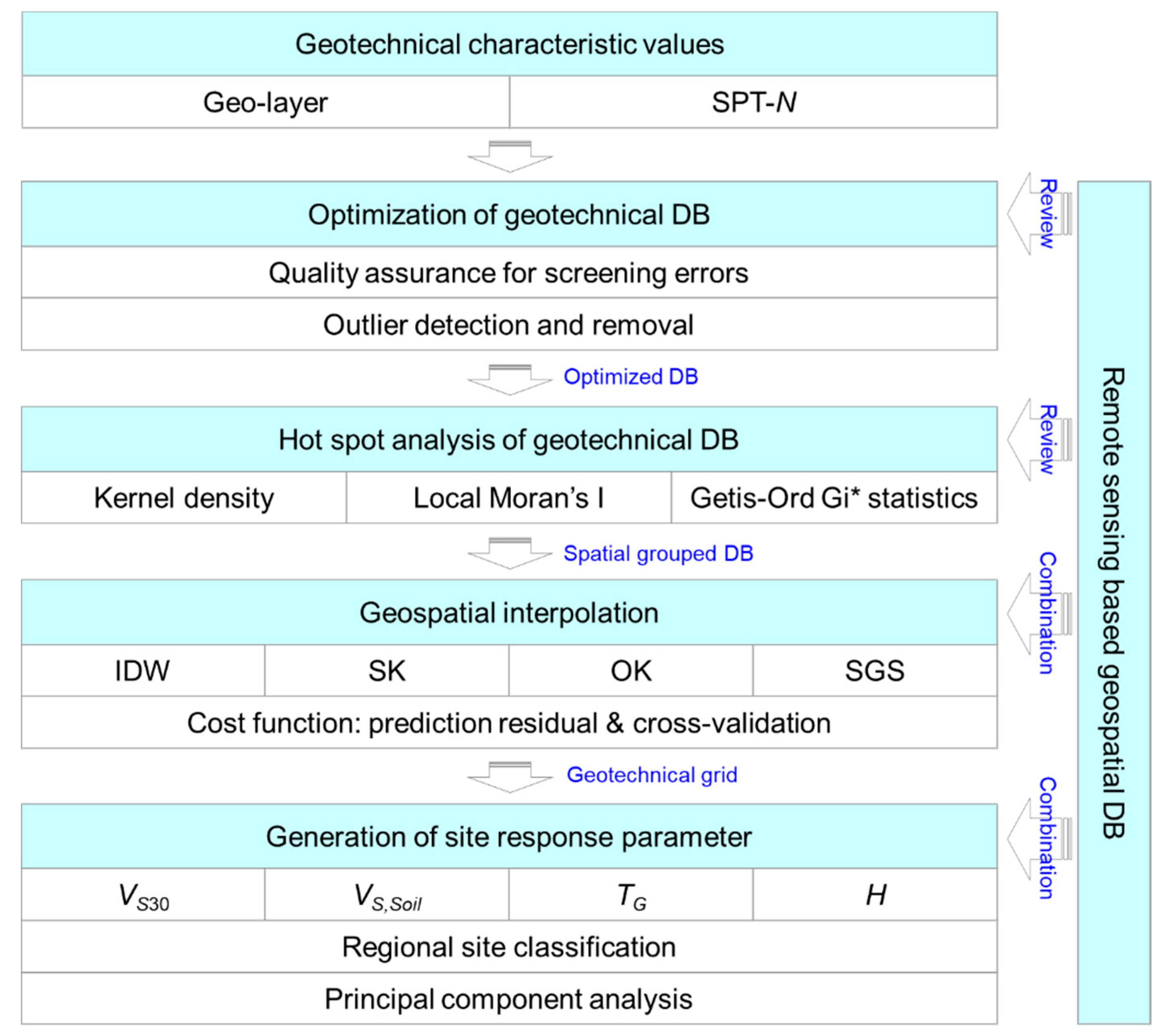
Figure 3.
Schematic showing procedures of geospatial characterization for regional seismic site classification.
Figure 3.
Schematic showing procedures of geospatial characterization for regional seismic site classification.
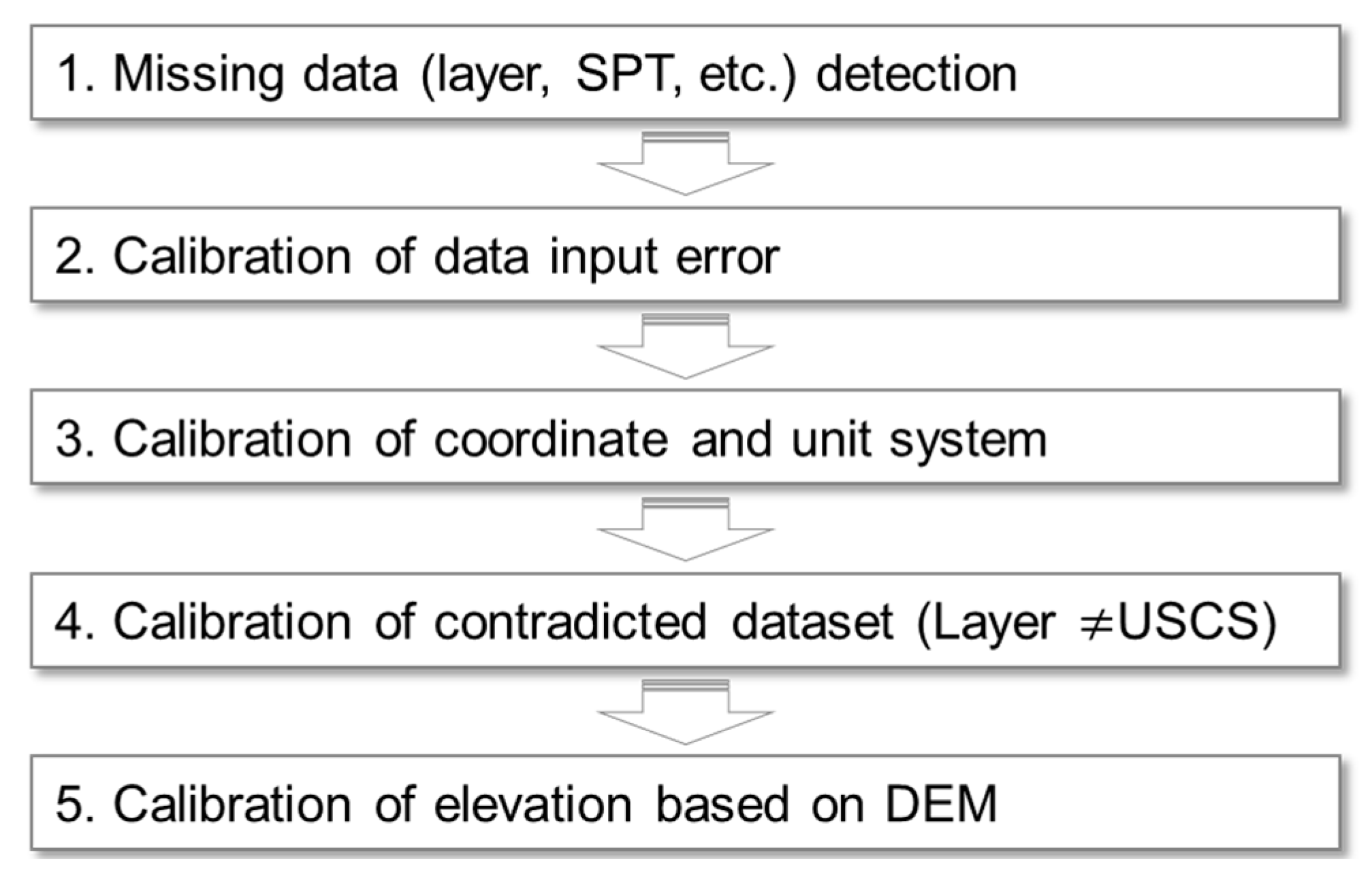
Figure 4.
Outlier detection of bedrock depth data in the borehole dataset based on (a) the cross-validation-based method, (b) Anselin Local Moran’s I statistic-based method, and (c) outliers detected by both methods, applied to bedrock depth. Outlier and clusters classified by Anselin Local Moran’s I statistic: NS (Not significant); H-H (High–High cluster); H-L (High–Low outlier); L-H (Low–High outlier); L-L (Low–Low cluster).
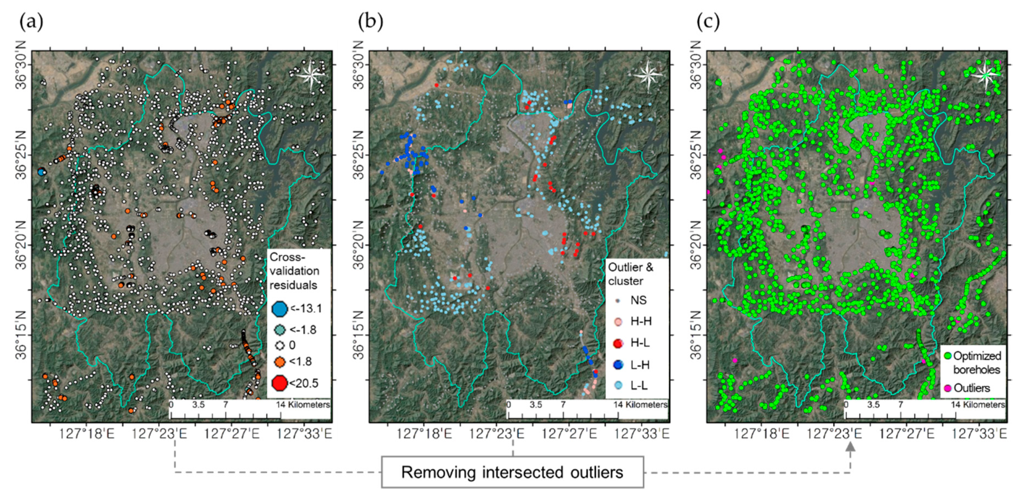
Figure 5.
Comparison of three hot spot analysis algorithms (Kernel Density, Local Moran’s I, and Getis-Ord Gi* statistics) applied to the engineering geo-layer thickness and average for fill layer; alluvial soil; weathered soil; weathered rock.
Figure 5.
Comparison of three hot spot analysis algorithms (Kernel Density, Local Moran’s I, and Getis-Ord Gi* statistics) applied to the engineering geo-layer thickness and average for fill layer; alluvial soil; weathered soil; weathered rock.
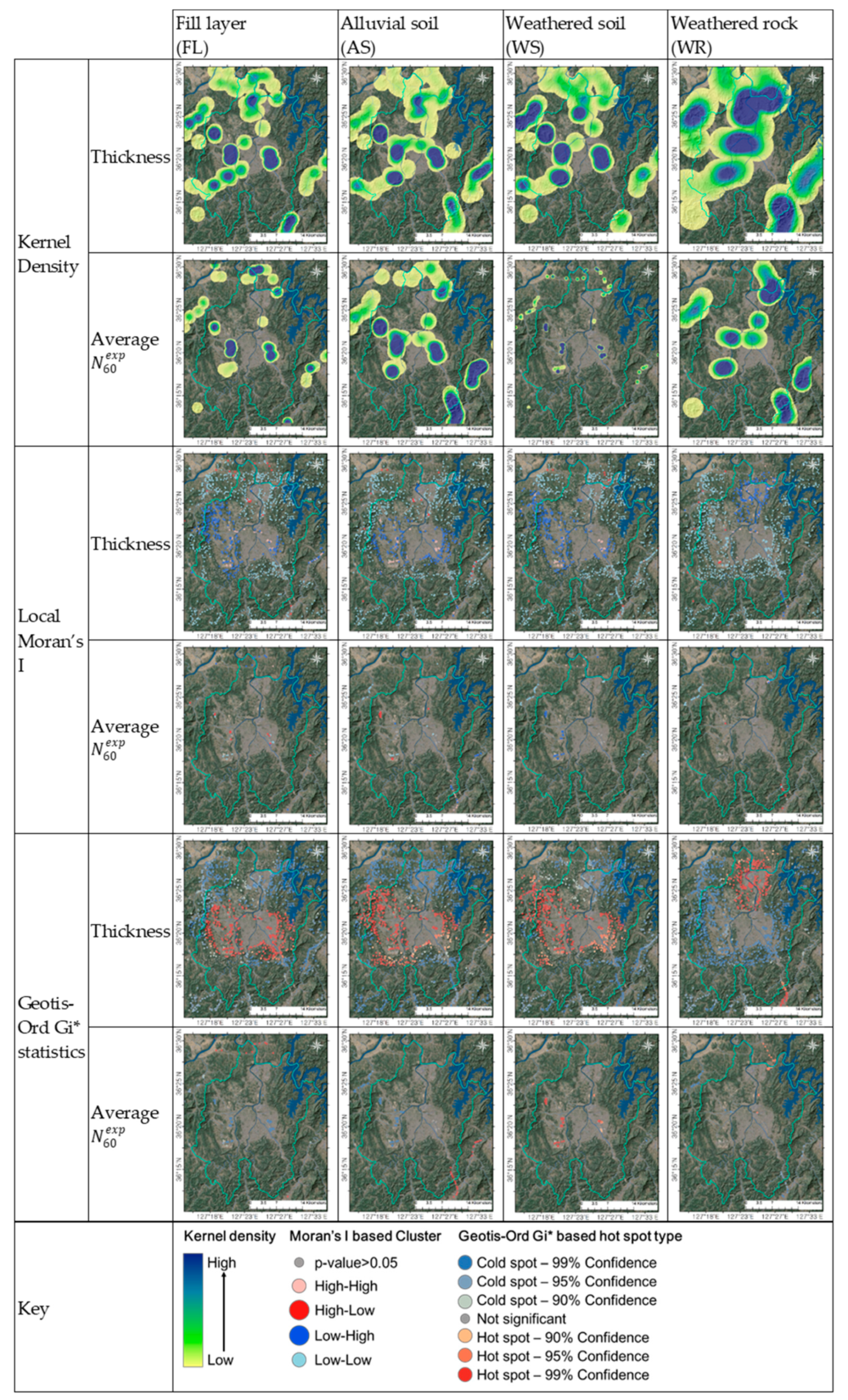
Figure 6.
Comparison of geospatial maps of engineering geo-layer thickness between different geostatistical interpolation algorithms including: Inverse Distance Weighting; Simple Kriging; Ordinary Kriging; Empirical Bayesian Kriging.
Figure 6.
Comparison of geospatial maps of engineering geo-layer thickness between different geostatistical interpolation algorithms including: Inverse Distance Weighting; Simple Kriging; Ordinary Kriging; Empirical Bayesian Kriging.

Figure 7.
Comparison of geospatial maps of average between different geostatistical interpolation algorithms including: Inverse Distance Weighting; Simple Kriging; Ordinary Kriging; Empirical Bayesian Kriging.
Figure 7.
Comparison of geospatial maps of average between different geostatistical interpolation algorithms including: Inverse Distance Weighting; Simple Kriging; Ordinary Kriging; Empirical Bayesian Kriging.
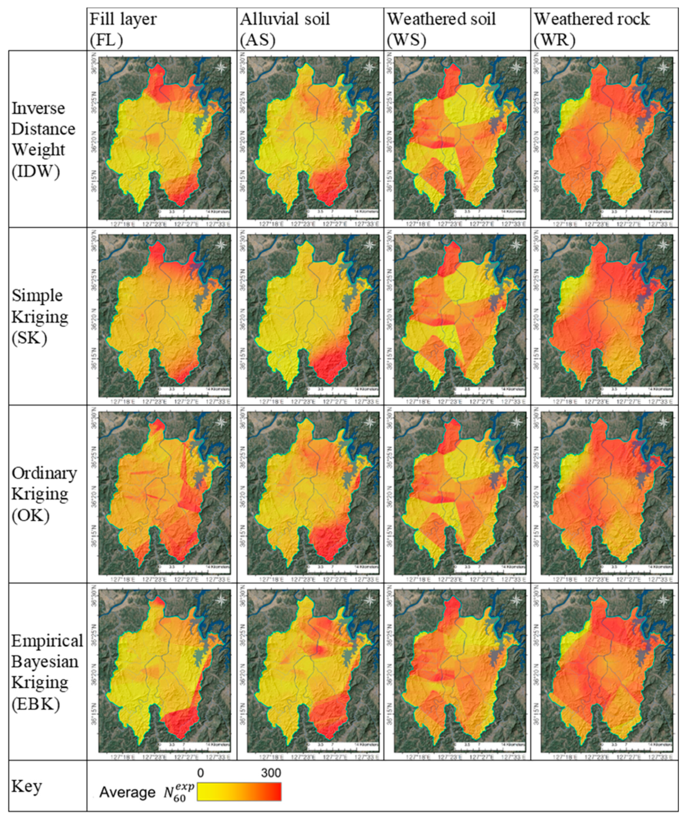
Figure 8.
Correlations between measured and predicted geo-layer thicknesses and correlations with measured and predicted average . The linear relations between measured and predicted values are shown by the dotted lines and summarized as tables. The residuals of prediction are shown by the blue lines.
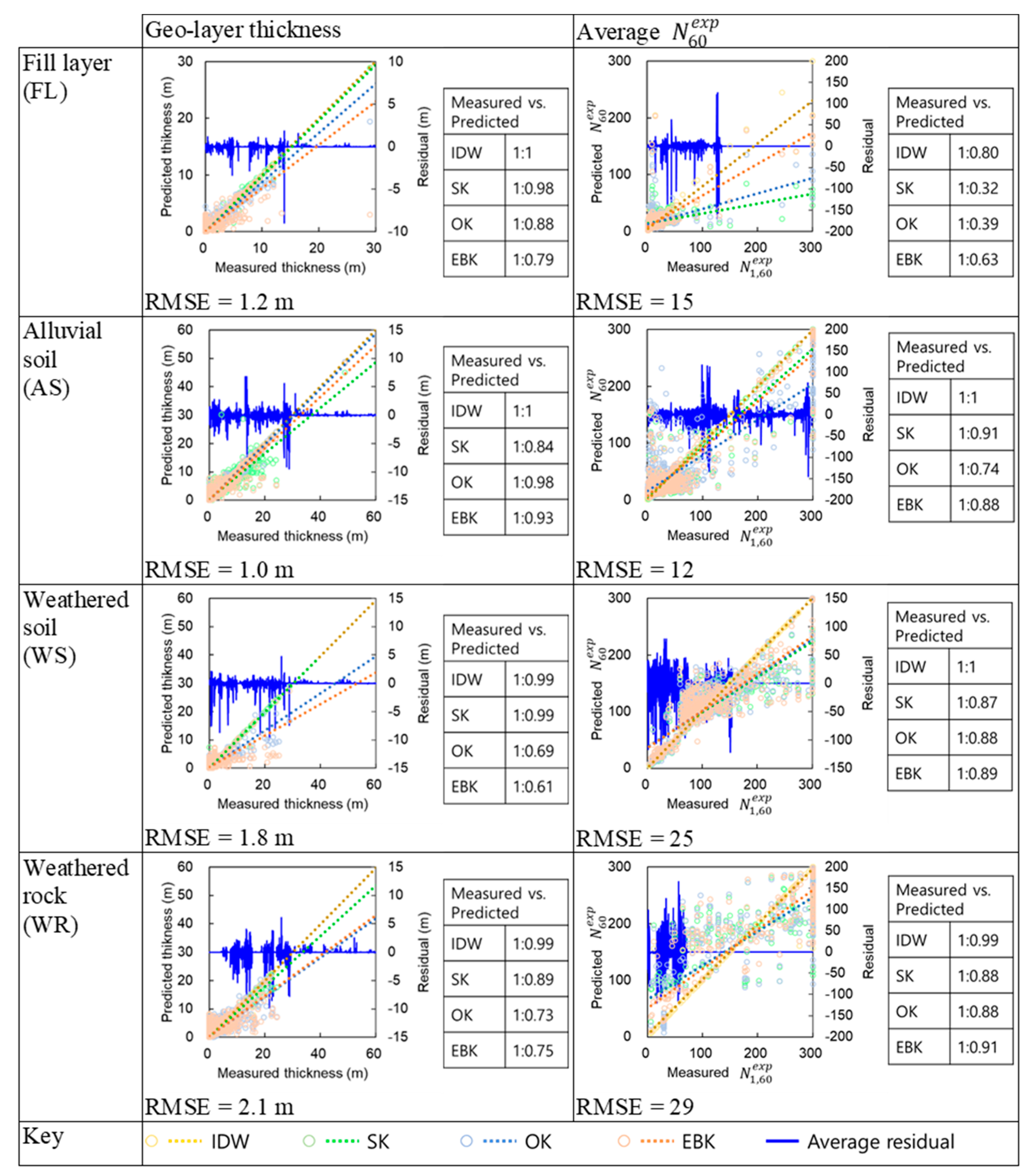
Figure 9.
Box plots of correlations between grid-based predicted geo-layer depth and average : (a) fill layer; (b) alluvial soil; (c) weathered soil; (d) weathered rock. The blue dotted lines show the regression line and equations with the highest R2.
Figure 9.
Box plots of correlations between grid-based predicted geo-layer depth and average : (a) fill layer; (b) alluvial soil; (c) weathered soil; (d) weathered rock. The blue dotted lines show the regression line and equations with the highest R2.
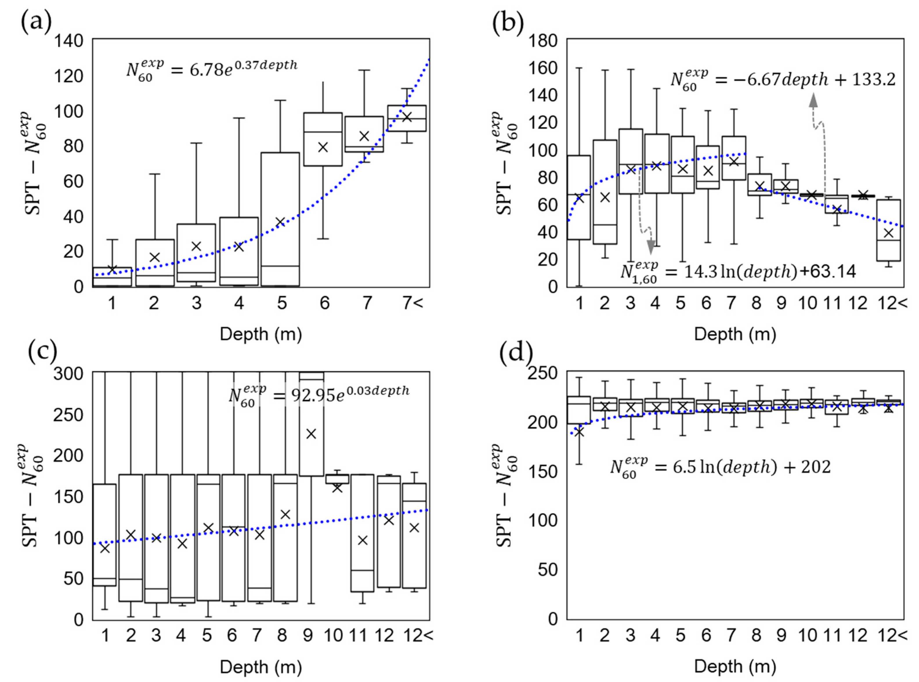
Figure 10.
Regional site classification of the seismic site effect parameters: (a) VS30; (b) TG; (c) H; and (d) the combination of VS,Soil and H based on MPSS 2017. VS30, TG, and H were categorized by Kim et al. [55].
Figure 10.
Regional site classification of the seismic site effect parameters: (a) VS30; (b) TG; (c) H; and (d) the combination of VS,Soil and H based on MPSS 2017. VS30, TG, and H were categorized by Kim et al. [55].

Figure 11.
Maps showing the results of using principal component analyses to unify the multilayer seismic zonation for the parameter combinations shown in Table 3: (a) combination #1; (b) combination #2; and (c) combination #3. (d) Map showing the seismic zonation with administrative sub-units generated using the average principal component-based site class (Table 1) and combination #3 for each clustered mesh.


Table 1.
Multivariate site classification system for seismic site effects (modified after Kim et al. [20]).
Table 1.
Multivariate site classification system for seismic site effects (modified after Kim et al. [20]).
| Generic Description | Site Class | Geotechnical Criteria | Geo-Proxy-Based Criteria | |||||||
|---|---|---|---|---|---|---|---|---|---|---|
| H (m) | VS30 (m/s) | TG (s) | f0 (Hz) | Slope (%) | Elevation (m) | Lithology | ||||
| Geological era | Stratigraphy | |||||||||
| Rock | B | <6 | >760 | <0.06 | >16.67 | >5.6 | >80 | Paleozoic | Plutonic/metamorphic rocks | |
| Weathered Rock and Very Stiff Soil | C | C1 | <10 | >620 | <0.10 | >10.00 | >3.5 | >60 | Mesozoic | Cretaceous fine-grained sediments |
| C2 | <14 | >520 | <0.14 | >7.14 | >2.0 | >45 | Weathered crystalline rocks | |||
| Intermediate Stiff Soil | C3 | <20 | >440 | <0.20 | >5.00 | >1.1 | >31 | Oligocene–Cretaceous sedimentary rocks | ||
| C4 | <29 | >360 | <0.29 | >3.45 | >0.62 | >22 | Oligocene coarse-grained younger material | |||
| Deep Stiff Soil | D | D1 | <38 | >320 | <0.38 | >2.63 | >0.23 | >18 | Cenozoic | Miocene fine-grained sediments |
| D2 | <46 | >280 | <0.46 | >2.17 | >0.08 | >14 | Coarse younger alluvium | |||
| D3 | <54 | >240 | <0.54 | >1.85 | >0.023 | >11 | Holocene alluvium | |||
| D4 | <62 | >180 | <0.62 | >1.61 | >0.006 | >9 | Fine-grained alluvial/estuarine deposits | |||
| Deep Soft Soil | E | ≥62 | ≤180 | ≥0.62 | ≤1.61 | ≤0.006 | ≤9 | - | Inter-tidal mud | |
Table 2.
Seismic site classification system of MPSS 2017 [64].
Table 2.
Seismic site classification system of MPSS 2017 [64].
| Site Class | Site Description | Parameters for Classification | |
|---|---|---|---|
| Bedrock 1 Depth, H (m) | VS,Soil (m/s) | ||
| S1 | Rock | H < 1 | - |
| S2 S3 | Shallow and stiff soil Shallow and soft soil | 1 ≤ H ≤ 20 | ≥260 m/s |
| <260 m/s | |||
| S4 | Deep and stiff soil | 20 < H | ≥180 m/s |
| S5 | Deep and soft soil | <180 m/s | |
| S6 | Special soil requiring site-specific evaluation | ||
1 Strata showing a shear wave velocity higher than 760 m/s.
Table 3.
Results of principal component analysis combinations for combined multivariate site response parameters.
Table 3.
Results of principal component analysis combinations for combined multivariate site response parameters.
| Component | Initial Eigen Value | Loading of Parameters | Percent of Eigen Value | Coefficient of Correlations | ||
|---|---|---|---|---|---|---|
| VS30 | TG | H | ||||
| Combination #1: VS30, TG | ||||||
| PC1 | 1.34 | 0.51 | 0.05 | - | 87.47 | 0.96 |
| PC2 | 0.19 | 0.25 | −0.12 | - | 10.53 | 0.61 |
| Combination #2: VS30, H | ||||||
| PC1 | 1.20 | 0.66 | - | 0.38 | 76.17 | 0.94 |
| PC2 | 0.37 | 0.16 | - | 0.75 | 11.83 | 0.11 |
| Combination #3: VS30, H, TG | ||||||
| PC1 | 1.36 | 0.75 | −0.07 | −0.16 | 70.95 | 0.94 |
| PC2 | 0.43 | 0.01 | 0.15 | −0.25 | 22.25 | 0.61 |
| PC3 | 0.13 | 0.25 | −0.19 | −0.04 | 6.80 | 0.44 |
Publisher’s Note: MDPI stays neutral with regard to jurisdictional claims in published maps and institutional affiliations. |
© 2020 by the authors. Licensee MDPI, Basel, Switzerland. This article is an open access article distributed under the terms and conditions of the Creative Commons Attribution (CC BY) license (http://creativecommons.org/licenses/by/4.0/).
Share and Cite
MDPI and ACS Style
Kim, H.-S.; Sun, C.-G.; Kim, M.; Cho, H.-I.; Lee, M.-G. GIS-Based Optimum Geospatial Characterization for Seismic Site Effect Assessment in an Inland Urban Area, South Korea. Appl. Sci. 2020, 10, 7443. https://doi.org/10.3390/app10217443
AMA Style
Kim H-S, Sun C-G, Kim M, Cho H-I, Lee M-G. GIS-Based Optimum Geospatial Characterization for Seismic Site Effect Assessment in an Inland Urban Area, South Korea. Applied Sciences. 2020; 10(21):7443. https://doi.org/10.3390/app10217443
Chicago/Turabian StyleKim, Han-Saem, Chang-Guk Sun, Mingi Kim, Hyung-Ik Cho, and Moon-Gyo Lee. 2020. "GIS-Based Optimum Geospatial Characterization for Seismic Site Effect Assessment in an Inland Urban Area, South Korea" Applied Sciences 10, no. 21: 7443. https://doi.org/10.3390/app10217443
Note that from the first issue of 2016, this journal uses article numbers instead of page numbers. See further details here.