Escaping Local Minima in Path Planning Using a Robust Bacterial Foraging Algorithm

Abstract

The bacterial foraging optimization (BFO) algorithm successfully searches for an optimal path from start to finish in the presence of obstacles over a flat surface map. However, the algorithm suffers from getting stuck in the local minima whenever non-circular obstacles are encountered. The retrieval from the local minima is crucial, as otherwise, it can cause the failure of the whole task. This research proposes an improved version of BFO called robust bacterial foraging (RBF), which can effectively avoid obstacles, both of circular and non-circular shape, without falling into the local minima. The virtual obstacles are generated in the local minima, causing the robot to retract and regenerate a safe path. The proposed method is easily extendable to multiple robots that can coordinate with each other. The information related to the virtual obstacles is shared with the whole swarm, so that they can escape the same local minima to save time and energy. To test the effectiveness of the proposed algorithm, a comparison is made against the existing BFO algorithm. Through the results, it was witnessed that the proposed approach successfully recovered from the local minima, whereas the BFO got stuck.

1. Introduction

The advancements in the field of robotics have a long history that dates back to the 1960s, when the first industrial robot was developed. Since then, many types of robots, such as humanoid robots, unmanned aerial vehicles (UAVs), unmanned water vehicles (UWVs), bio-inspired robots, sci-fi robots, and unmanned ground vehicles (UGVs) more commonly known as mobile robots, found their applications in various fields [1,2,3,4]. One of the key areas where robots are extensively used is exploration and monitoring. For the purpose, mobile robots are mainly utilized due to their affordability and maneuverability. Realistically, all mobile robots are supposed to maneuver in their surroundings in the presence of obstacles. Therefore, path planning (PP) is considered the most critical task that defines the success or failure of the whole process.

Robots are usually equipped with multiple input sensors and decision-making control systems in order to traverse through a trajectory, which can be foreknown or determined online. It is desired that robots be capable enough to avoid complex obstacles while online or offline. The degree of severity is multiplied many times for unknown cluttered environments [5,6]. The environment is perceived through different sensors, such as ultrasonic sensors, laser range finders, and cameras. To avoid the obstacles, the most common approach is to control the heading angle of the mobile robot in order to steer away. There are many algorithms that help robots to perform such actions; some are preferred over others based upon their performances. In the field of PP, some researchers have focused on the development of intelligent mobility strategies that enable mobile robots to explore both static and dynamic environments independently [7]. There can exist multiple paths that lead to the target. The selection of an optimal path is usually dependent upon the satisfaction of some constraints or rules, such as shortest distance, least energy consumption, and minimum time. Among these, the cost function based upon displacement is considered the most important due to its effectiveness in almost all situations [8]. Therefore, the overall optimization problem can be posed as the determination of the path that ensures the shortest distance from the start to the end point.

Rapidly-exploring random trees, probabilistic roadmaps [9], genetic algorithms [10,11,12], neural networks, simulated annealing [13], particle swarm optimization [14,15], ant colony optimization [16], and bacterial foraging optimization [17,18] to name a few, belong to the wide class of heuristic and meta-heuristic algorithms [19]. These methods have their own advantages and disadvantages. For over a decade, mathematical programming, cell decomposition, roadmap, and the artificial potential field (APF) have been considered as handy tools to perform motion planning. APF is still considered as one of the most common and reliable planning techniques [20]; however, it provides only one trajectory that may not be optimal necessarily. APF received much attention after the work of Khatib et al., who worked upon obstacle avoidance in an effective manner [21]. It has also been shown in [22] that potential fields can be utilized for controlling robot swarm formation, collision prevention, and swarm motion. The artificial field generated around the mobile robot comprises two main forces: the attractive potential field force that attracts the robot to the goal point, and the repulsive potential field force that repels the robot away from any obstacle’s field. The total potential field of APF is generated when both forces are combined (attractive + repulsive) [23]. APF is considered an effective navigation approach, but it suffers from a local minima problem. When the amounts of attractive and repulsive forces acting on robot become equal, its movement is ceased unless some external effect is applied. Recently, [24] proposed an improved version of APF, where they employed the concept of reward and penalty as in reinforcement learning (RL). More precisely, an additional force is introduced that helps the robot to avoid the local minimum.

From a wide class of PP algorithms, BFO, proposed by [25], is relatively new and has a lot of potential as it can find an optimal path quite effectively. Using this path, a robot can prevent obstacles in the workspace, hence ensuring maximum safety. BFO is a simple and effective bio-inspired method of optimization that has solved many issues of engineering and mobile robotics, including problems related to PP [26]; however, the solution is not always guaranteed. Ideally, BFO can encounter only single local minima, located at the desired configuration. In practice though, it can run into situations where the attractive and repulsive forces can produce local minima at unknown locations. The robot cannot estimate local minima in an unobserved environment. In other words, the simple control strategy based upon gradient may or may not converge to the goal. The local minima correspond to the local valleys, where the robot can get stuck. Avoidance of a local minimum in BFO has also been explored by some researchers; e.g., the authors in [27] claimed that the considered potential functions do not require gradient computation, and thereby do not suffer from local minima. An enhanced BFO proposed by [28] demonstrated that the mobile robot successfully avoids both static and dynamic obstacles. In a similar work [17], some authors explored the inherent characteristics of BFO in order to suggest an improved version of the basic BFO. However, most of these solutions only considered circular obstacles in order to support their claim. There is a strong chance that these approaches may not be able to avoid the local minima whenever non-circular obstacles are encountered.

The main impetus of this work was to devise a PP strategy that has the ability to avoid being trapped in local minima whenever non-circular shaped obstacles are encountered in an unknown environment. For that purpose, a virtual obstacle is introduced to assist the robot in escaping a local minimum. The number of virtual obstacles is dependent upon the size of the obstacle. The proposed robust bacterial foraging (RBF) algorithm, can be thought of as an extension to the work of [17,18]. Most existing works consider only the circular obstacles; therefore, the escape from local minima is not guaranteed against non-circular shaped obstacles. The proposed approach is quite reliable and is less complex; hence, it can be used for real-time PP. Additionally, the given approach can be extended to a swarm of robots, where the virtual obstacles’ information is exchanged among them in order to reduce time and error. The major contributions of this paper are three-fold:

• A unique idea of virtual obstacles is introduced that effectively helps the robots to recover from the local minima;
• The information about the virtual obstacles is shared among the whole swarm and can be utilized to pre-plan the route without conflicting with the same local minima;
• The proposed strategy is not computationally intensive; therefore, it can be easily utilized in real-time applications.

The remainder of the paper is organized as follows. Section 2 covers the basic knowledge about APF and BFO in order to better understand the proposed approach. The generation of an optimal path using the proposed algorithm is discussed in Section 3. Simulation results are displayed in Section 4 to validate the proposed approach, and brief concluding remarks and potential future topics are given in the last section.

2. Preliminaries

This section is devoted to a brief review about the artificial potential field and bacterial foraging optimization that form the basis for the proposed work.

2.1. Artificial Potential Field (APF)

The artificial potential field has established itself as one of the most desirable approaches due to its being easy to understanding [29]. The robot is identified as an object that is driven by the field of forces. An attractive force generated by the target attracts the robot and it is repelled by the repulsive force generated by the obstacles. This two-force combination is devoted to the control of robot’s movement in a safer environment while avoiding obstacles.

2.1.1. Attractive Potential

The attractive potential field is generated for driving the robot to the target location. The general idea is to increase the attractive $U_{att}\left(q\right)$ field as the robot moves away from the goal. Among many mathematical functions, the quadratic potential, Equation (1), is used for this study:

$$U_{att}\left(q\right)=\frac{1}{2}{K}_{att}{∥q_g-q∥}^2$$

(1)

where $K_{att}>0$ is used to control the scaling; $q_g={\left[x_g,y_g\right]}^T$ is the location of the goal; $q={\left[x,y\right]}^T$ is the location of the robot; and $∥q_g-q∥$ is the Euclidean distance between the robot and the goal. The force exerted by the goal is defined as the negative gradient of the attractive potential function [21].

$$F_{att}\left(q\right)=-\nabla U_{att}\left(q\right)=-\frac{\partial U_{att}\left(q\right)}{\partial q}=-K_{att}(q-q_g)$$

(2)

$F_{att}\left(q\right)$ has two components: along the x-axis and the y-axis.

2.1.2. Repulsive Potential

The repelling force generated by the obstacles is used to maintain a safe distance between the robot and the obstacles; however, if the robot stays outside the safe region defined around the obstacles, its motion remains unaffected. The repulsive potential field for each $ith$ obstacle has the following relation:

$$U_{re{p}_i}\left(q\right)=\{\begin{array}{c}\frac{1}{2}{K}_{rep}{\left(\frac{1}{d_i\left(q\right)}-\frac{1}{d_o}\right)}^2,\mathrm{if}{d}_i\left(q\right)\le d_o\hfill \\ 0,\mathrm{otherwise}\hfill \end{array}$$

(3)

where $K_{rep}>0$ is used for scaling, $d_o$ is the range to define the obstacle’s influence, and $d_i\left(q\right)$ is the distance from the robot to the closest point in each individual obstacle. The repulsive force is the negative gradient of the repulsive potential function [21]:

$$F_{re{p}_i}\left(q\right)=-\nabla U_{re{p}_i}\left(q\right)$$

(4)

$$F_{re{p}_i}\left(q\right)=\{\begin{array}{c}{K}_{rep}\left(\frac{1}{d_i\left(q\right)}-\frac{1}{d_o}\right)\left(\frac{1}{d_i^2\left(q\right)}\right)\nabla d_i\left(q\right),\mathrm{if}{d}_i\left(q\right)\le d_o\hfill \\ 0,\mathrm{otherwise}\hfill \end{array}$$

(5)

where

$$\nabla d_i\left(q\right)=\frac{q-q_c}{∥q-q_c∥}$$

$q_c={\left[x_c,y_c\right]}^T$ is the position of the closest point in the $ith$ obstacle. Similarly to $F_{att}\left(q\right)$, $F_{rep}\left(q\right)$ also has two components: along the x-axis and the y-axis. If the environment contains n obstacles, then the total repulsive potential field is:

$$U_{rep}\left(q\right)=\sum _{i=1}^n{U}_{re{p}_i}\left(q\right)$$

(6)

2.1.3. Total Potential

Once the attractive and the repulsive potential functions are obtained, the total potential function can be determined by summing both forces:

$$U\left(q\right)=U_{att}\left(q\right)+\sum _{i=1}^n{U}_{re{p}_i}\left(q\right)$$

(7)

Thus, the resultant potential force is:

$$F\left(q\right)=-\nabla U\left(q\right)=F_{att}\left(q\right)+\sum _{i=1}^n{F}_{re{p}_i}\left(q\right)$$

(8)

2.2. Bacteria and Bacterial Foraging Optimization

The human brain is difficult to understand and it is very hard to build a machine of this complexity. For this reason, researchers have turned their efforts towards easy organisms and micro-organisms, such as bacteria, which are very delicate organisms each consisting of only one cell, usually several micrometers in length. For handling, locating, and ingesting food, a bacterium’s foraging strategies are quite simple, yet effective. The basic foraging mechanism of Escherichia coli provides the basis for the whole process. Some bacteria have high chances of reproducing due to their strong foraging strategy, whereas those with weaker strategies may end up eliminated. Those that survive must struggle for the maximization of the energy obtained per unit time. This whole problem is formulated as an optimization problem that determines the optimal foraging decisions. Sometimes these decisions are associated with the maximization of long-term energy subject to some constraints, such as absence of complete information (e.g., limited sensing capability) and the risks involved. Such optimization approaches strive for the construction of an optimal controller (policy) for making foraging decisions. The same knowledge of optimal foraging formulation is then extended to the field of robotics.

Assumption 1.

The differential drive robot considered is from the broad class of wheeled mobile robots (WMRs). It is assumed that the moving frame is associated with the robot to update its position and heading angle in a 2-D plane, whose information is available throughout.

Assumption 2.

In this study, it is considered that the sensing capability of the robot is limited; therefore, it can only sense the obstacles or other robots when it reaches their vicinity.

3. Implementation Details

In this research, BFO is exploited to seek an efficient solution for mobile robots. The rationale behind the selection of bacterial foraging is its robustness against the area of the workspace and nonlinearity, and it can handle more objective functions when compared to other evolutionary algorithms.

3.1. The Robot’s Trajectory Process

With the bacterial foraging algorithm, the process is initialized by generating $N_s$ random particles (bacterium) around the robot within a circle of radius R. This defines the step size of the movement in the trajectory as:

$${\theta }^i(t+dt)={\theta }^i\left(t\right)+R\left(\frac{\Delta \left(t\right)}{∥\Delta \left(t\right)∥}\right)$$

(9)

where $\Delta \left(t\right)$ is a random vector of a unit length to determine the direction of each particle, and $∥\Delta \left(t\right)∥$ defines the magnitude of the vector. Each bacterial group that is around the robot keeps searching for the optimal way to the target, and it can change direction at any time. The robot updates its position to that of one of these bacteria based on the selection of the best. This process continues until every obstacle is avoided and the goal is reached. The determination of the strongest bacterium is based upon two considerations. At every step, the distance between each bacterium, and the distance between the current position of the robot and the nearest obstacle, are calculated. The application of these two variables results in an attractive-repellent pattern, which guides the robot to the target point (global minimum).

During the movement of the robot, the cost function $J_o$ is zero when no obstacle is encountered. Otherwise, it will assume the repulsive Gaussian cost function for an obstacle:

$$J_o=\{\begin{array}{c}{H}_{o}ex{p}^{-W_o{∥{\theta }^i\left(t\right)-q_o\left(t\right)∥}^2},\mathrm{if}∥q_o\left(t\right)-q∥\le \beta \hfill \\ 0,\mathrm{otherwise}\hfill \end{array}$$

(10)

$H_o$ and $W_o$ are constants that refer to the repellent’s height and width, respectively. With sensors placed at the front of the robot, it can detect any obstacle’s location, $q_o\left(t\right)$. The value of the $J_o$ always remains zero until the robot senses the obstacle in its range, whereas the range of the sensor can be adjusted by $\beta$. The Gaussian cost function of the goal point can be represented as:

$$J_g=-H_{g}ex{p}^{-W_g{∥{\theta }^i\left(t\right)-q_g\left(t\right)∥}^2}$$

(11)

$H_g$ and $W_g$ refer to the goal’s height and width. The direct distance between the goal and the $ith$ bacterium can be calculated by the Euclidean distance, $∥{\theta }^i\left(t\right)-q_g\left(t\right)∥$. Obstacle avoidance and goal search are the two most important concerns during mobile robots’ PP. For the purpose, a combined cost function is defined as:

$$J=J_o+J_g$$

(12)

The above equation is used to find the total cost of each bacterium. Based upon their cost values, all particles are sorted from highly desirable to undesirable. Then, the robot’s current location, $q\left(t\right)$, is updated according to the highly desirable $ith$ bacterium that ensures the minimum possible cost. These steps will guide the robot to the target while avoiding the obstacles. The strategy is based on the distance error, which can be written as follows:

$$e_d^i=d^i(t+dt)-d^i\left(t\right)$$

(13)

where $d^i\left(t\right)$ and $d^i(t+dt)$ are the Euclidean distances from the $ith$ bacterium’s position ${\theta }^i$ to the goal $q_g$ at times t and $t+dt$, respectively. Equation (14) is the cost function error used for sorting all bacteria in an ascending order. The particle with the lowest distance error will be at the top of the priority list.

$$e_J^i\left(t\right)=J\left({\theta }^i(t+dt)\right)-J\left({\theta }^i\left(t\right)\right)$$

(14)

The robot keeps on saving the trajectory in its memory; this information is later used for avoiding the local minima and rerouting.

3.2. Different Shapes of Obstacles

The bacterial foraging optimization algorithm does not always guarantee success when different types of obstacles are encountered. Unfortunately, with some types of obstacles, the robot can get stuck in the local minima which can cause failure of this algorithm. There are many types of obstacles a robot can face on its path which need to be avoided. Practically, it is difficult to know beforehand whether the robot will be stuck in a local minimum or not. The main focus of this study is to develop an improved version of the bacterial foraging algorithm to bypass multiple types of obstacles without falling into a local minimum.

3.3. Robust Bacterial Foraging (RBF) Algorithm

With RBF, the robot takes one step at a time and records these steps in a temporary memory. The target location always attempts to attract the robot, whereas the obstacle always tries to push the robot away. If a robot is stuck in a local minimum, it will stop for a while and save its current position $p_{vo}$ and the number of iterations j in the memory. At this position, a virtual obstacle is generated whose information is conveyed to the swarm. Using this information, other robots can continue smooth travel without falling into local minima. The distance between the robot’s current location—the same as the position of the virtual obstacle—and each point in its trajectory is then calculated. Thereafter, the robot chooses a point from an available set that has a specific distance (constant distance) and moves back to it with the help of an additional repulsive function. Once the robot returns to a certain point from its path, it again starts traveling towards the target, along which it might encounter another obstacle in the surroundings.

The start and the target locations for the mobile robot are assumed as $(q_s,q_g)$, where $d_{min}$ is defined as the radius of the field used to determine the location of the goal. The population of bacteria around the robot in each step is represented by $N_s$, where $l_p$ represents the iteration that helps the mobile robot to save its trajectory. When the robot falls in a local minimum, it chooses one of the points in its trajectory that has a specific distance, $dis$, and moves back to it. The location of the robot is represented by q. The number of virtual obstacles that the robot creates when it falls into a local minimum is denoted by $l_o$ (Algorithm 1).

Algorithm 1 Pseudocode of the robust bacterial foraging (RBF) algorithm.

Input: $q_s,q_g,d_{min},N_s,dis$ Procedure: Initialize robot position, $q\leftarrow q_s;$ $l_o\leftarrow 1;l_p\leftarrow 0;i\leftarrow 0;j\leftarrow 0;$ $d\leftarrow ∥q-q_g∥;$ while $\left(d\ge d_{min}\right)$     $l_p\leftarrow l_p+1;$     while$i\le N_s$        generate random bacterium $N_s$ around q in radius $R;$        use Equation (9) to calculate the next point;        use Equations (10)–(12) to calculate $J_o$, $J_g$, and $J;$        compute error using Equations (13) and (14);        $i\leftarrow i+1;$     endwhile     $i\leftarrow 0;$     sort cost function error in Equation (14);     select best bacterium;     $q\leftarrow bestpoint;$     save the trajectory, $T\left(l_p\right)\leftarrow q;$     if robot falls in local minima then        $p_{vo}\leftarrow q;$        $j\leftarrow l_p;$        while $∥q-T\left(j\right)∥\le dis$            $j\leftarrow j-1;$        endwhile        $virobstale\left(l_o\right)\leftarrow p_{vo};$        $l_o\leftarrow l_o+1;$        use additional cost function in Equation (15) to reach a specific trajectory        point, $q\leftarrow T\left(j\right);$     endif     update $d;$ endwhile Output: Location of the virtual obstacles and trajectory of the robot.

3.4. Local Minima Criterion

The actual trajectory of the robot is stored in T and it keeps on updating itself according to the robot’s current location $q\left(t\right)$. It is assumed that the robot is being trapped in the local minimum if no movement is sensed for a defined time, i.e., $\sum _k\left|q\left(t\right)-q(t+kdt)\right|<S$. $dt$ is the time step, k is used to define the number of observations, and S is chosen as a minimum distance that the robot covers in one time step. Once it is confirmed that a local minimum has been encountered, then a virtual obstacle is generated at the same location. From the stored trajectory, a point is chosen based upon $dis$. An additional repulsive Gaussian cost function is created for the virtual obstacle:

$$J_{add}=H_{add}ex{p}^{-W_{add}{∥q\left(t\right)-T\left(j\right)∥}^2}$$

(15)

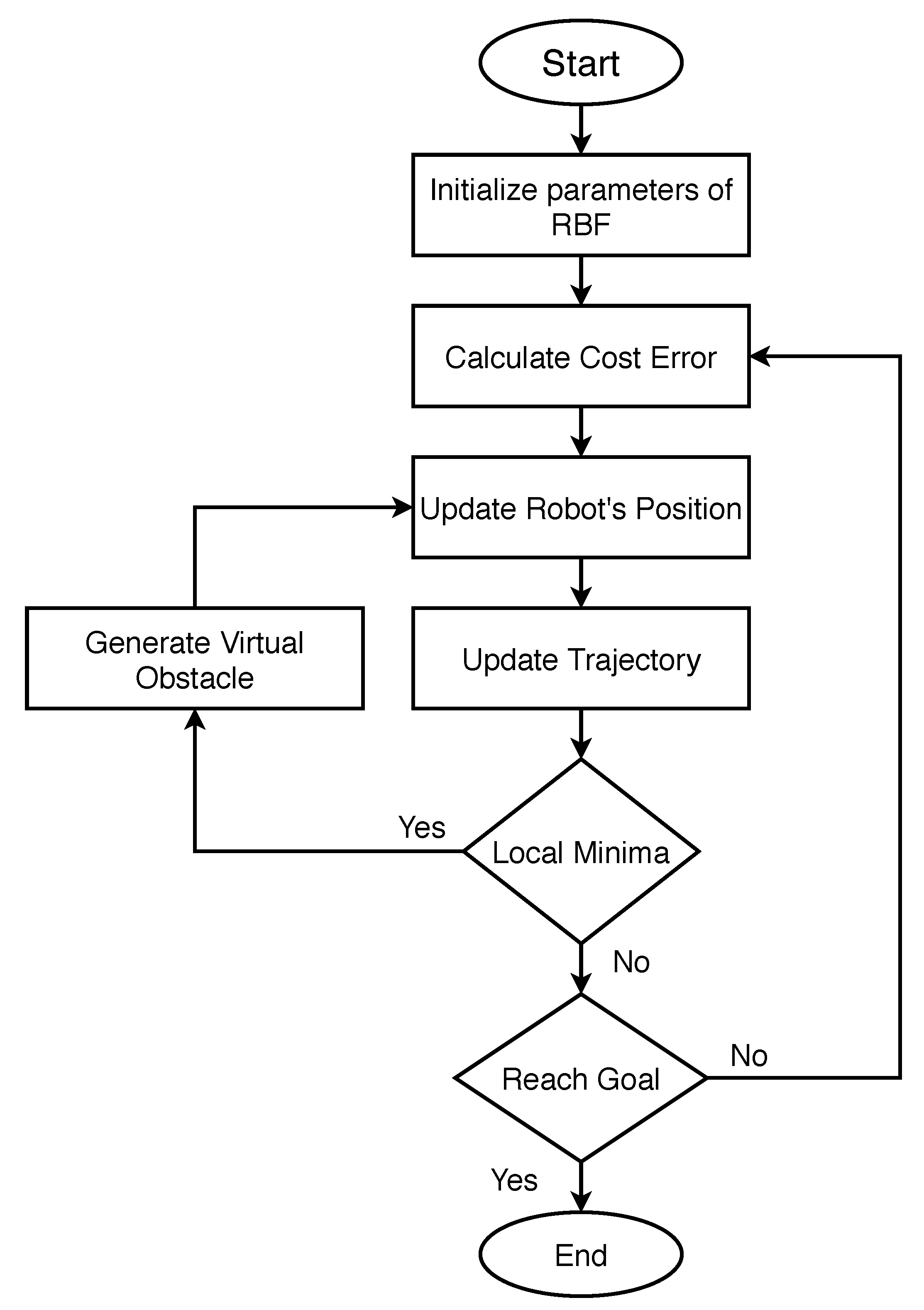
where $H_{add}$ and $W_{add}$ are used to define the height and width of the virtual obstacle. This cost function is only effective when the robot falls into a local minimum; moreover, its effect keeps on decreasing as it approaches the desired point on the trajectory. In order to generate a cumulative effect, $J_{add}$ is added to the cost functions in Equation (12). The flow chart of the entire process is depicted in Figure 1.

4. Results and Discussion

In order to validate the proposed approach, two different scenarios with different environments were simulated using MATLAB 2020a. A differential drive robot was used for the simulation, whose kinematic parameters were adapted from [30]. Three ultrasonic sensors, used for determining the obstacles, were affixed to the front of the mobile robot. In this study, based on assumption 2, the range of the sensor was limited and defined as 13 cm. The results were obtained for a mobile robot performing navigation in a cluttered environment with different types of obstacles in a 2-D workspace.

4.1. Scenario 1: Cases without Local Minima Problem

In this scenario, the robot faces circular obstacles in three different configurations. The purpose is to approach the target without hitting the obstacles.

4.1.1. Case 1: Static and Moving Obstacle

The target is defined at (−20, 90) and the robot starts to travel from (50, −90), as shown in Figure 2. The robot continues its travel on a pre-determined path till it senses the presence of an obstacle on its path. The task is to approach the target location without any collisions. In Figure 2, the robot successfully reaches the target by rerouting in order to avoid a circular static obstacle. It is worth mentioning that the location of the obstacle was not known. The repulsive Gaussian cost function forces the robot to pick the farthest bacterium from the obstacle that lies at the boundary of the sensing range. Due to this constraint, the robot keeps on moving alongside the boundary till it re-approaches the defined path.

A dynamic obstacle is also considered, which moves on a horizontal plane at a constant speed of 5.217 cm/s. The situation is depicted in Figure 3, where the robot’s movement is registered at four different time instances. It can be observed easily that until the robot reaches the vicinity of the obstacle and senses its presence, its motion remains unaffected. The robot resumes its travel on the same course when the obstacle passes away and cannot be sensed any further. During this process, the RBF keeps on generating new particles around the robot to search for a better solution. The robot’s movement is confined due to the obstacle; therefore, generation of the new particles is limited to a very small region. The elapsed time required to reach the target is about 11.86 s. The total cost function in each step of the robot is the sum of $J_o$, $J_g$, and $J_{add}$ of all the particles around the robot. The next candidate particle is the one having the lowest cost function error. The repellent Gaussian cost function is maximal only if the robot is near the obstacle, and zero if it cannot sense the influence of the obstacle.

4.1.2. Case 2: Three Obstacles Intercepting the Path

In this case, three obstacles are placed close to each other in such a way that the robot cannot pass through. As shown in Figure 4, the robot successfully escaped all the obstacles and reached the goal. It was observed that the robot sensed the repellent zone around the obstacles and rerouted itself. This zone helps the robot to maintain its safe distance from the physical obstacles. If due to high speed the robot accidentally enters the safe zone, retraction is made until the safe distance is attained. The required convergence time for this case is 8.98 s. The repellent Gaussian cost function is highest near the obstacles. There is absolutely no repulsive effect on the robot if the distance between the robot and the obstacles is more than the defined threshold.

4.1.3. Case 3: An Obstacle on a Direct Path

In this case, the obstacle is intentionally placed in the robot’s trajectory toward the target. The robot is able to reroute itself as soon as it senses the presence of the obstacle. For a short while, it continues its journey on the boundary of the safe zone defined by the obstacle. As soon as it gets away from the repellent force of the obstacle, it redefines its course towards the goal point, as shown in Figure 5. Due to the generation of the random particles around the robot, its behavior is not fixed, and can change from trial to trial. We noticed that on some occasions, the robot bypassed the obstacle from the left side.

In other methods, such as potential field, the robot gets trapped in a local minimum because the existence of the attractive and the repulsive forces on the same line nullify each other’s effect. Consequently, the robot gets stuck and stays at one place indefinitely, yet the proposed algorithm effectively solves the problem by avoiding the local minima and causing the robot to reach the target.

4.2. Scenario 2: Cases with Local Minima Problem

The local minima problem usually emerges when the robot encounters multiple circular obstacles or non-circular obstacles. Four such cases are defined where robot(s) face circular and non-circular shaped obstacles.

4.2.1. Case 1: Two Circular-Shaped Obstacles Lying Close to Each Other

In this case, shown in Figure 6, the target is defined at (−20, 90), the obstacles are located at (10, 50) and (−10, 50), and the robot is initialized from (50, −90). The obstacles are positioned intentionally so that they can obstruct the robot’s trajectory. The robot cannot pass through the obstacles due to its physical limitation and the safe zone defined around the obstacles. The resultant field generated by the two obstacles prevents the robot from moving towards the target. The robot’s movement was observed for $kdt$ time instances. If the distance traveled was shorter than the defined threshold, then the robot was regarded as trapped in a local minimum. A virtual obstacle was generated at this trap point, and with the help of the virtual obstacle’s cost function, the robot was repelled. The robot chose one of the points from the stored trajectory that had a specific distance from its current position and moved back to that point. Later, it resumed its journey towards the goal where the virtual obstacle was detected before the actual obstacle and it caused the robot to correct its heading in order to avoid obstacles and approach the target.

4.2.2. Case 2: L-Shaped Obstacle

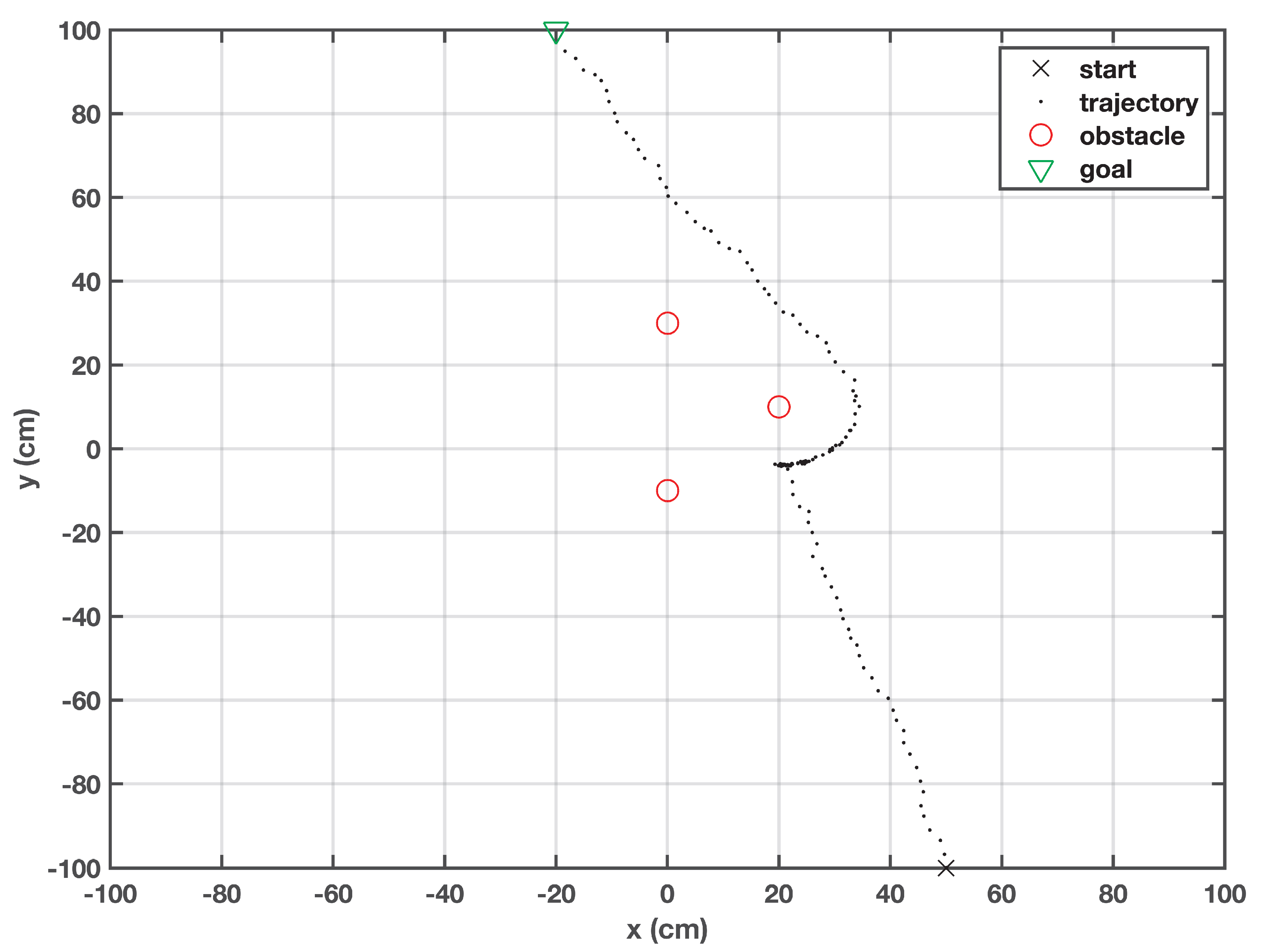
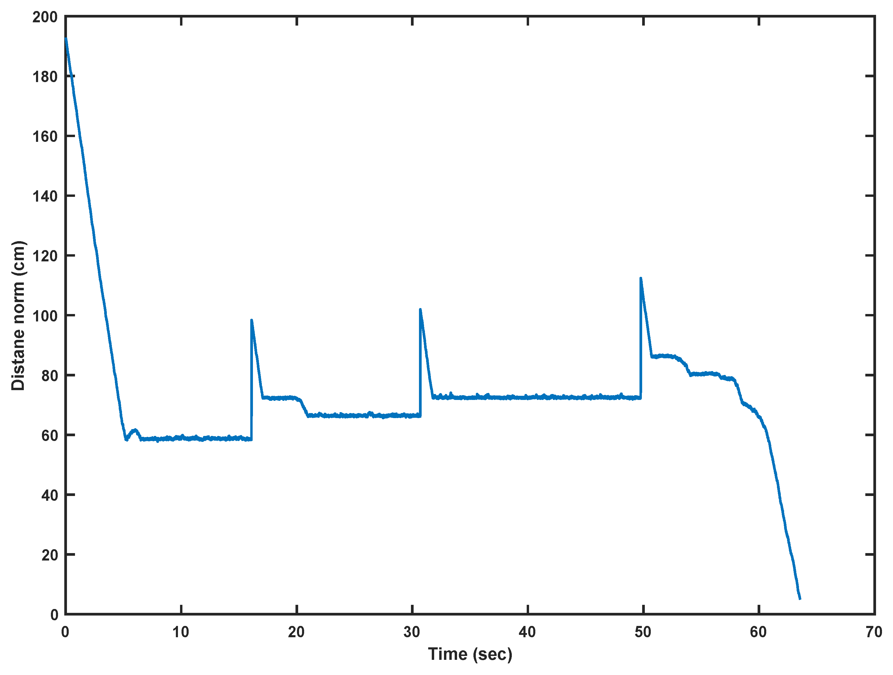
A trickier type of obstacle is the L-shaped obstacle, which is usually used as a test case for PP algorithms. For this scenario (Figure 7), the target was defined at (−20, 90) and the robot was initialized at (50, −90). As expected, the robot fell into a local minimum; then it created a virtual obstacle, as shown in Figure 7. This obstacle is responsible for providing the robot with a certain push, so that it can reach a certain point on the stored trajectory. The robot fell into a local minimum three times; hence, the same number of virtual obstacles were generated. After recovering from a local minimum, it resumed its travel towards the target. It is noticed that the robot kept changing its direction every time it faced a virtual obstacle. The distance norm (Euclidean distance) between the target and the current position of the robot is plotted against time and shown in Figure 8. Upon the creation of each virtual obstacle, the robot retracts and readjusts itself; it causes the spikes in the distance norm plot. It is noticeable that there is no bound on the number of virtual obstacles; therefore, RBF can keep on generating the virtual obstacles every time the robot is trapped. However, if the robot is surrounded by virtual obstacles, then it is regarded as an irrecoverable state.

4.2.3. Case 3: U-Shaped Obstacle

The proposed algorithm was evaluated for the U-shaped obstacles—probably the trickiest regular-shaped obstacles. On the course to the target, the robot fell into a local minimum nine times, as shown in Figure 9. It is noticed that the virtual obstacles created by the robot were arranged in a regular shape, and the distances among virtual obstacles were uniformly divided. The robot overcame the non-circular obstacles by creating virtual obstacles, so that it could move sufficiently enough from the original obstacle. Once an open path was available, the robot corrected its heading in order to approach the target. After minor adjustments in its heading, the robot was able to reach the target in a successful manner.

4.2.4. Case 4: Virtual Obstacles’ Information Exchange among the Robots

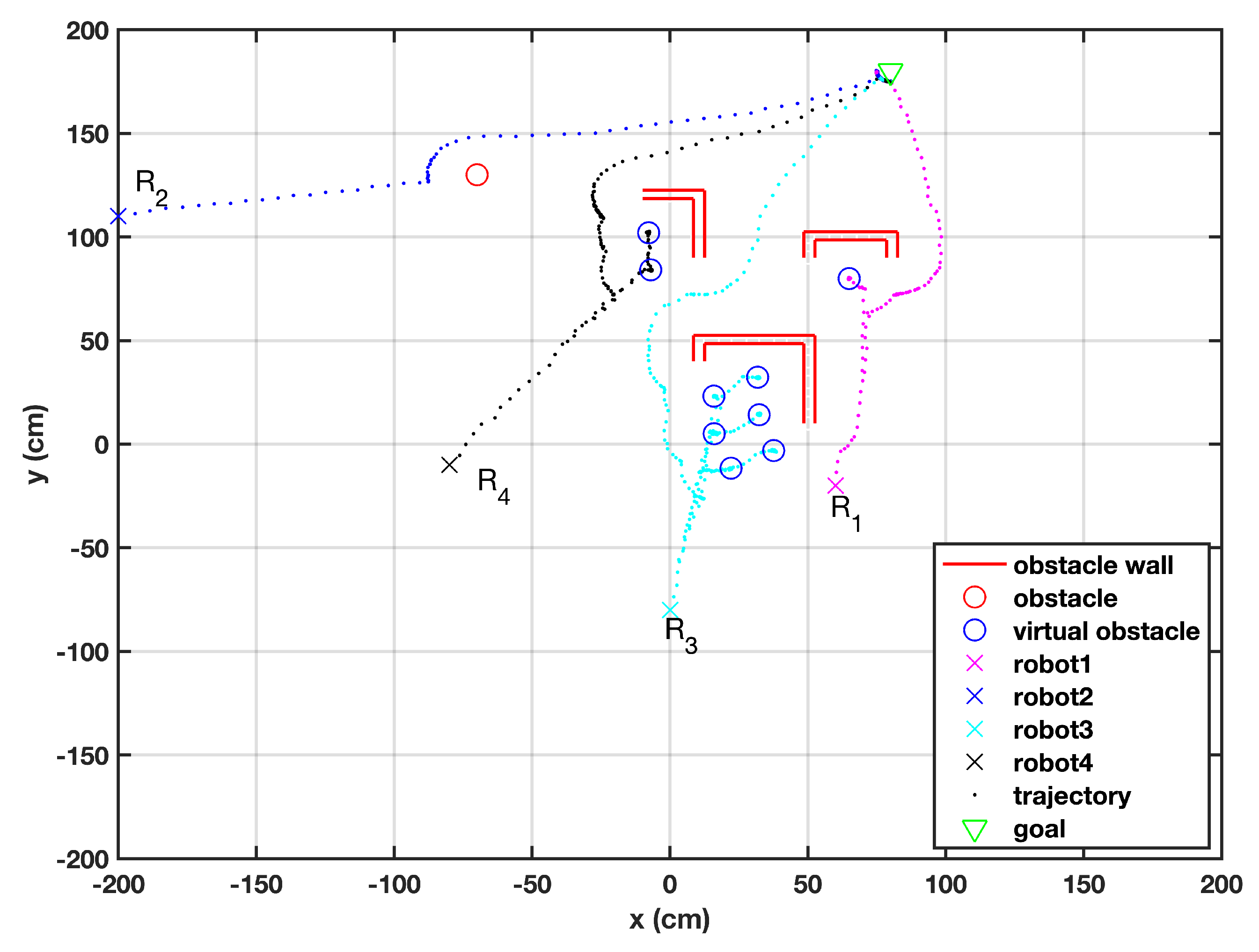
The methodology of the proposed algorithm can be easily extended to a swarm of robots. In this case, four robots are initialized from different locations facing differently shaped obstacles, shown in Figure 10. When one of the robots falls in a local minimum, it creates a virtual obstacle and shares this information with other robots to prevent them from falling into the same local minimum. For instance, the information about the virtual obstacles defined by robot $R_4$ is conveyed to the whole swarm. $R_3$ uses this information to avoid being trapped in the same local minimum and reroutes itself in a timely manner. Hence, it is unnecessary to scan one obstacle more than once.

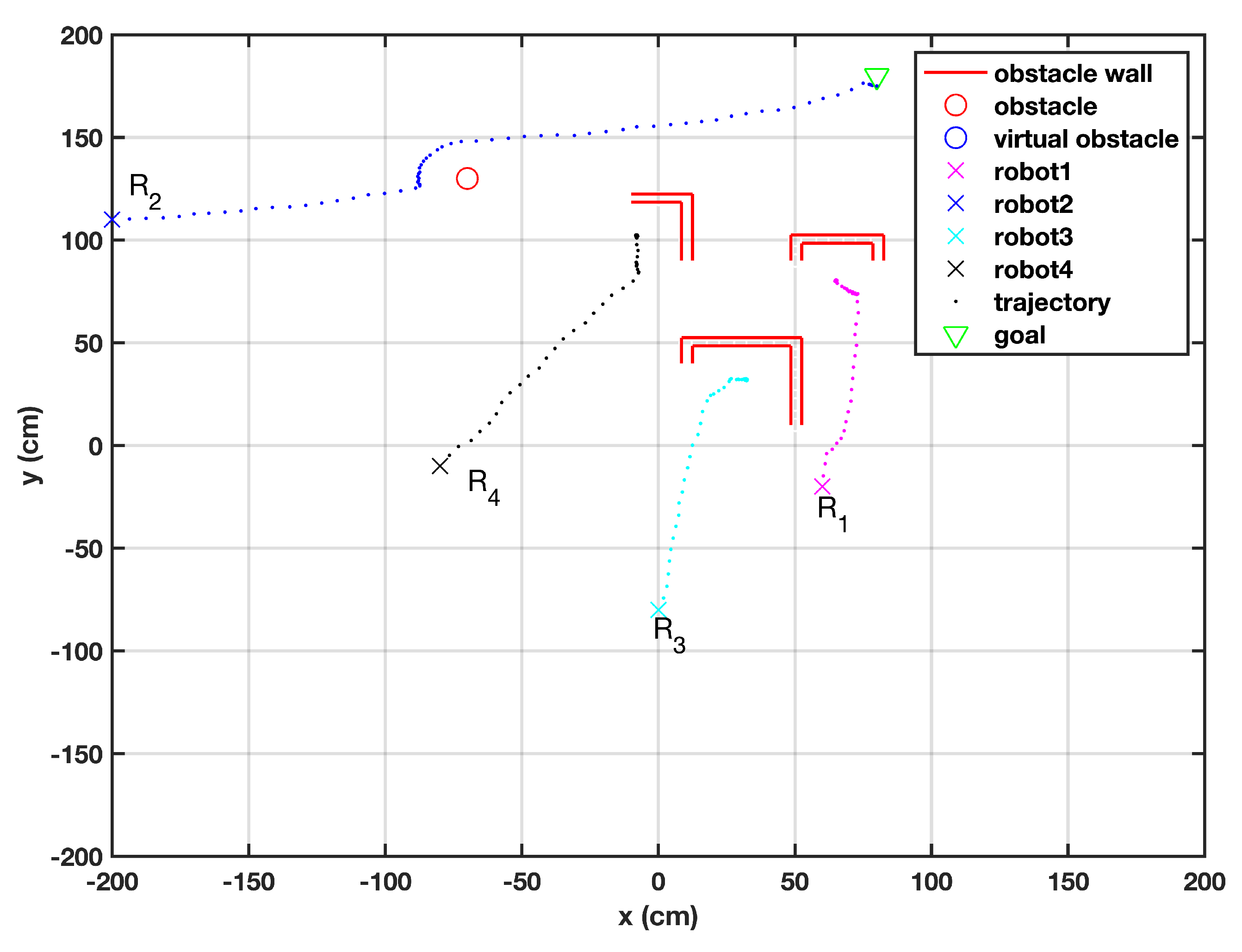
The performance of the proposed algorithm is compared against the work of [17]. It is illustrated in Figure 11 that three robots failed to reach the target and fell into local minima, from where they could not recover. The robots $R_2$, $R_3$, and $R_4$ got trapped in the local minima of the wall-shaped obstacles, while $R_1$ successfully overcame the circular obstacle; that is a relatively easier type of obstacle. This proved that the proposed algorithm, based upon its robust performance, has been able to outperform its predecessor algorithm.

5. Conclusions and Future Work

The prime objective of this work was to approach the target in an effective manner while avoiding differently shaped obstacles. The proposed algorithm, robust bacterial foraging (RBF), was developed to be more effective and reliable as compared to the existing work. The BFO algorithm is considered effective only against circular obstacles. Therefore, this work can be considered as an extension to the existing BFO, as it enhances the range to differently shaped obstacles in order to extend the capability. The algorithm uses the input data from multiple ultrasonic sensors installed on the front of the robot to identify the environment, the locations of the obstacles, and the bearing of the target position. The decision scheme permits the robot to choose its next position from a number of bacteria around it. The information about the explored obstacles is distributed to the whole swarm, which in turn uses this information to pre-plan its trajectory to reduce time and error. Through the results, it can be claimed that the proposed algorithm proved its efficiency and high performance in many scenarios with unknown environments.

Though the proposed approach has been able to perform well in most cases, there are still two scenarios considered topics of future interest, wherein the algorithm requires additional testing:

• When the starting point is near a local minimum or over a local minimum, the robot becomes unable to return to a specific distance placed in its memory; hence, it stops moving;
• When the robot encounters a closed-form obstacle, it keeps on generating virtual obstacles in order to avoid the actual obstacle. Doing so fills the space with virtual obstacles, disrupting the forward motion.

References

- Goldhoorn, A.; Garrell, A.; Alquézar, R.; Sanfeliu, A. Searching and tracking people with cooperative mobile robots. Auton. Robot. 2018, 42, 739–759. [Google Scholar] [CrossRef] [Green Version]
- Ando, H.; Ambe, Y.; Ishii, A.; Konyo, M.; Tadakuma, K.; Maruyama, S.; Tadokoro, S. Aerial hose type robot by water jet for fire fighting. IEEE Robot. Autom. Lett. 2018, 3, 1128–1135. [Google Scholar] [CrossRef]
- Muijzert, E.; Welker, K.E. Seismic Data Acquisition Using Water Vehicles. U.S. Patent 10,191,170, 29 January 2019. [Google Scholar]
- Mende, M.; Scott, M.L.; van Doorn, J.; Grewal, D.; Shanks, I. Service robots rising: How humanoid robots influence service experiences and elicit compensatory consumer responses. J. Mark. Res. 2019, 56, 535–556. [Google Scholar] [CrossRef]
- Khan, M.U.; Li, S.; Wang, Q.; Shao, Z. CPS oriented control design for networked surveillance robots with multiple physical constraints. IEEE Trans. Comput.-Aided Des. Integr. Circuits Syst. 2016, 35, 778–791. [Google Scholar] [CrossRef]
- Khan, M.U.; Li, S.; Wang, Q.; Shao, Z. Formation control and tracking for co-operative robots with non-holonomic constraints. J. Intell. Robot. Syst. 2016, 82, 163–174. [Google Scholar] [CrossRef]
- Pandey, A.; Pandey, S.; Parhi, D. Mobile robot navigation and obstacle avoidance techniques: A review. Int. Rob. Auto. J. 2017, 2, 00022. [Google Scholar] [CrossRef] [Green Version]
- Abbas, N.H.; Ali, F.M. Path planning of an autonomous mobile robot using directed artificial bee colony algorithm. Int. J. Comput. Appl. 2014, 96, 11–16. [Google Scholar]
- Kavraki, L.E.; Svestka, P.; Latombe, J.; Overmars, M.H. Probabilistic roadmaps for path planning in high-dimensional configuration spaces. IEEE Trans. Robot. Autom. 1996, 12, 566–580. [Google Scholar] [CrossRef] [Green Version]
- Berger, J.; Jabeur, K.; Boukhtouta, A.; Guitouni, A.; Ghanmi, A. A hybrid genetic algorithm for rescue path planning in uncertain adversarial environment. In IEEE Congress on Evolutionary Computation; IEEE: Piscataway, NJ, USA, 2010; pp. 1–8. [Google Scholar]
- Li, S.; Ding, M.; Cai, C.; Jiang, L. Efficient path planning method based on genetic algorithm combining path network. In Proceedings of the Fourth International Conference on Genetic and Evolutionary Computing, Shenzhen, China, 13–15 December 2010; IEEE: Piscataway, NJ, USA, 2010; pp. 194–197. [Google Scholar]
- Hocaoglu, C.; Sanderson, A.C. Planning multiple paths with evolutionary speciation. IEEE Trans. Evol. Comput. 2001, 5, 169–191. [Google Scholar] [CrossRef]
- Zhang, K.; Collins, E.G.; Barbu, A. An efficient stochastic clustering auction for heterogeneous robotic collaborative teams. J. Intell. Robot. Syst. 2013, 72, 541–558. [Google Scholar] [CrossRef] [Green Version]
- Kennedy, J.; Eberhart, R. Particle swarm optimization. In Proceedings of the ICNN’95—International Conference on Neural Networks, Perth, Australia, 27 November–1 December 1995; Volume 4, pp. 1942–1948. [Google Scholar]
- Alam, M.S.; Rafique, M.U.; Khan, M.U. Mobile robot path planning in static environments using particle swarm optimization. arXiv 2020, arXiv:2008.10000. [Google Scholar]
- Montiel-Ross, O.; Sepúlveda, R.; Castillo, O.; Melin, P. Ant colony test center for planning autonomous mobile robot navigation. Comput. Appl. Eng. Educ. 2013, 21, 214–229. [Google Scholar] [CrossRef]
- Hossain, M.A.; Ferdous, I. Autonomous robot path planning in dynamic environment using a new optimization technique inspired by bacterial foraging technique. Robot. Auton. Syst. 2015, 64, 137–141. [Google Scholar] [CrossRef]
- Das, S.; Biswas, A.; Dasgupta, S.; Abraham, A. Bacterial Foraging Optimization Algorithm: Theoretical Foundations, Analysis, and Applications. In Foundations of Computational Intelligence Volume 3: Global Optimization; Abraham, A., Hassanien, A.E., Siarry, P., Engelbrecht, A., Eds.; Springer: Berlin/Heidelberg, Germany, 2009; pp. 23–55. [Google Scholar] [CrossRef]
- Mac, T.T.; Copot, C.; Tran, D.T.; De Keyser, R. Heuristic approaches in robot path planning: A survey. Robot. Auton. Syst. 2016, 86, 13–28. [Google Scholar] [CrossRef]
- Tsuji, T.; Tanaka, Y.; Morasso, P.G.; Sanguineti, V.; Kaneko, M. Bio-mimetic trajectory generation of robots via artificial potential field with time base generator. IEEE Trans. Syst. Man Cybern. Part C (Appl. Rev.) 2002, 32, 426–439. [Google Scholar] [CrossRef] [Green Version]
- Khatib, O. Real-Time Obstacle Avoidance for Manipulators and Mobile Robots; Springer: New York, NY, USA, 1986; pp. 396–404. [Google Scholar]
- Barnes, L.E.; Fields, M.A.; Valavanis, K.P. Swarm formation control utilizing elliptical surfaces and limiting functions. IEEE Trans. Syst. Man Cybern. Part B (Cybern.) 2009, 39, 1434–1445. [Google Scholar] [CrossRef]
- Lee, M.C.; Park, M.G. Artificial potential field based path planning for mobile robots using a virtual obstacle concept. In Proceedings of the IEEE/ASME International Conference on Advanced Intelligent Mechatronics (AIM), Kobe, Japan, 20–24 July 2003; IEEE: Piscataway, NJ, USA, 2003; Volume 2, pp. 735–740. [Google Scholar]
- Wu, Q.; Chen, Z.; Wang, L.; Lin, H.; Jiang, Z.; Li, S.; Chen, D. Real-Time Dynamic Path Planning of Mobile Robots: A Novel Hybrid Heuristic Optimization Algorithm. Sensors 2020, 20, 188. [Google Scholar] [CrossRef] [Green Version]
- Passino, K.M. Biomimicry of bacterial foraging for distributed optimization and control. IEEE Control Syst. Mag. 2002, 22, 52–67. [Google Scholar]
- Coelho, L.D.S.; Sierakowski, C.A. Bacteria colony approaches with variable velocity applied to path optimization of mobile robots. ABCM Symp. Ser. Mech. 2006, 2, 2972–3304. [Google Scholar]
- Mohajer, B.; Kiani, K.; Samiei, E.; Sharifi, M. A new online random particles optimization algorithm for mobile robot path planning in dynamic environments. Math. Probl. Eng. 2013, 2013, 49134. [Google Scholar] [CrossRef] [Green Version]
- Abbas, N.H.; Ali, F.M. Path planning of an autonomous mobile robot using enhanced bacterial foraging optimization algorithm. Al-Khwarizmi Eng. J. 2016, 12, 26–35. [Google Scholar] [CrossRef]
- Dunias, P. Autonomous Robots Using Artificial Potential Fields. Ph.D. Thesis, Technische Universiteit Eindhoven, Eindhoven, The Netherlands, 1996. [Google Scholar]
- Cook, G. Mobile Robots: Navigation, Control and Remote Sensing; John Wiley & Sons: Hoboken, NJ, USA, 2011. [Google Scholar]
Figure 1.
Flowchart of the proposed RBF algorithm.
Figure 2.
Trajectory of the robot when a static obstacle is encountered.
Figure 3.
Trajectory of the robot when a moving obstacle is encountered.
Figure 4.
Trajectory of the robot when three obstacles are encountered.
Figure 5.
Trajectory of the robot when the obstacle lies straight ahead.
Figure 6.
Behavior of the robot when local minima is encountered due to the close obstacles.
Figure 7.
Behavior of the robot when L-shaped obstacle is encountered.
Figure 8.
Distance norm calculated between the robot’s position and target.
Figure 9.
Behavior of the robot when U-shaped obstacle is encountered.
Figure 10.
A swarm of robots facing individual obstacles of different shapes.
Figure 11.
A swarm of robots facing individual obstacles [17].
Publisher’s Note: MDPI stays neutral with regard to jurisdictional claims in published maps and institutional affiliations. |
© 2020 by the authors. Licensee MDPI, Basel, Switzerland. This article is an open access article distributed under the terms and conditions of the Creative Commons Attribution (CC BY) license (http://creativecommons.org/licenses/by/4.0/).
Share and Cite
MDPI and ACS Style
Abdi, M.I.I.; Khan, M.U.; Güneş, A.; Mishra, D. Escaping Local Minima in Path Planning Using a Robust Bacterial Foraging Algorithm. Appl. Sci. 2020, 10, 7905. https://doi.org/10.3390/app10217905
AMA Style
Abdi MII, Khan MU, Güneş A, Mishra D. Escaping Local Minima in Path Planning Using a Robust Bacterial Foraging Algorithm. Applied Sciences. 2020; 10(21):7905. https://doi.org/10.3390/app10217905
Chicago/Turabian StyleAbdi, Mohammed Isam Ismael, Muhammad Umer Khan, Ahmet Güneş, and Deepti Mishra. 2020. "Escaping Local Minima in Path Planning Using a Robust Bacterial Foraging Algorithm" Applied Sciences 10, no. 21: 7905. https://doi.org/10.3390/app10217905
Note that from the first issue of 2016, this journal uses article numbers instead of page numbers. See further details here.