Droop Control Strategy of Utility-Scale Photovoltaic Systems Using Adaptive Dead Band


1
School of Electrical Engineering, Korea University, 145 Anam-ro, Seongbuk-gu, Seoul 02841, Korea
2
Energy ICT Convergence Research Department, KIER, 152, Gajeong-ro, Yuseong-gu, Daejeon 34129, Korea
*
Author to whom correspondence should be addressed.
Appl. Sci. 2020, 10(22), 8032; https://doi.org/10.3390/app10228032
Submission received: 27 September 2020
/
Revised: 4 November 2020
/
Accepted: 9 November 2020
/
Published: 12 November 2020
(This article belongs to the Special Issue Renewable Energy Systems 2020)
Abstract
:This paper proposes a novel droop control strategy for addressing the voltage problem against disturbance in a transmission system connected with a utility-scale photovoltaic. Typically, a voltage control at the renewable energy sources (RESs) connected to the transmission grid uses a reactive power–voltage control scheme with a fixed dead band. However, this may cause some problems; thus, this paper proposes a method for setting a dead band value that varies with time. Here, a method for calculating an appropriate dead band that satisfies the voltage maintenance standard for two disturbances is described using voltage sensitivity analysis and the equation of existing droop control. Simulation studies are conducted using the PSS® E program to analyze the short term voltage stability and display the results for various dead bands. The proposed modeling and operational strategy are validated in simulation using a modified IEEE 39 bus system. The results provide useful information, indicating that the control scheme through an adaptive dead band enables more stable system operation than that through a fixed dead band.
1. Introduction
Recently, a wide range of sustainable energy policies have been implemented in several countries to increase the share of electricity generation from renewable energy sources (RESs). Broad-based policies, such as tradable energy certificates, are more likely to induce innovation in RES’ technologies that are close to competitive with conventional generators. In particular, carbon emission issues can be resolved using RESs, such as photovoltaic (PV) and wind power, and an increase in the number of RESs shifts the system topology from large-scale generations to distributed generations (DGs) [1]. However, the rapid increase in DGs can cause various power system stability issues [2], including system inertia reduction [3], transmission congestion [4], substation overload [5], and voltage fluctuation [6]. In particular, the voltage problem caused by randomly generated output power from climate-affected DGs is the main concern for system operators.
The integration of a DG with high variability in a conventional network may create a voltage problem [7,8]. Regarding voltage regulation in transmission systems, several coordination strategies have been proposed so far, which can be classified into two groups: (1) coordinated control between DGs and reactive power compensation facilities, such as a flexible AC transmission system (FACTS) [9,10], and (2) supplementary control functions, which have been implemented for DGs to use the advanced reactive power–voltage control method [11,12,13]. To achieve advanced control ability, previous studies have focused on decentralized and centralized control strategies [14,15,16,17].
The decentralized control method acquires network data (e.g., bus voltage magnitude) at the point of interconnection (POI), and if the measuring voltage does not meet the reliability criteria, the individual parameters of DGs are set to compensate the voltage error and adjust the voltage set point within an acceptable range. The basic approach to implementing decentralized control of DGs is to use the sensitivity method [18,19]. Sensitivity cannot be calculated online without the communication infrastructure, such as the phasor monitoring unit, and the method used to calculate sensitivity using the Jacobian matrix incurs large calculation time. Thus, the authors in [20] presented improved decentralized control with a surface fitting technique in offline studies, where multiple DGs were coordinated by the time delay setting technique to perform accurate voltage control. However, these methods are less accurate because the two control strategies cannot consider the sudden network topology change caused by a rapid change in the RES output power. Moreover, the primary control objectives in the no-feedback control and grid-connected modes of operation are conflicting. The decentralized droop controllers force only the bus voltages to deviate from their nominal values in the primary control, because the current standard employs proportional control loops locally at each inverter. This causes voltage fluctuations, especially under an asymmetrical fault. Furthermore, the system voltage is adjusted by adding a control function that matches the allowable voltage to individual DGs, rather than through interaction with other DGs or facilities in the system.
In the centralized method, the control signal is transmitted to DGs and other reactive power resources by the central controller through a communication system, and is optimized for better voltage regulation. For example, model predictive control was used to reduce the modeling inaccuracies and measurement noise of facilities in a distribution system [21], which can be applied in transmission systems. In that study, a cooperative control for DGs and the load tap changer (LTC) was proposed to regulate the voltage to be within the allowable range. However, the LTC action takes a few seconds per tap to move, and thus, is not reasonable for controlling the power electronics-interfaced DGs, which can rapidly change the output power. In [22,23], multiple devices were used to counteract the uncertain voltage fluctuations using the multi-timescale method. For example, capacitor banks and on-load tap changers with slow and discrete responses were dispatched every hour without information on stochastic renewable output and load variation. The inverter interfaced with the DGs adjusted the reactive power output by checking the uncertainty every 15 min. However, depending only on probability distribution in the dispatch algorithm, an inaccurate control may occur in the sudden network topology change.
In the centralized control method with a transmission system operator (TSO) [24], a voltage fluctuation was detected by an accurate state estimation scheme within the control center of the TSO. TSOs contain information about the network state, and thus, can check for voltage limit violation for changes in load or RES output and take appropriate action. Another approach that uses a multiagent system (MAS) for intelligent volt/var control in power systems was proposed in [25,26,27]. MAS enables autonomous control of local distribution energy resources through a centralized energy management system (EMS) [5]. In addition, using this system, it is possible to not only maintain the voltage profile but also minimize the system loss and switching times of shunt capacitors [25]. Although the method using MAS with EMS suggests an optimal use of system devices, all reactive power resources must communicate with all other resources or a central controller, thus requiring network observability and a dense communication architecture. In addition, these MAS approaches require the parameters and operation points to be updated every time the network state changes; moreover, the complex nonlinearities of power and voltage in the optimal power flow model make the problem-solving time-consuming. Thus, the present paper proposes an adaptive dead band strategy, which is a simpler and more intuitive control strategy than the previously proposed ones.
Most of the previously proposed reactive power–voltage control strategies for transmission systems have many drawbacks compared to the proposed method. Decentralized coordination control methods [21,23], which perform voltage regulation in power systems, are less accurate than the proposed method. To increase the accuracy of the sensitivity method [18,19,20], historical information regarding DG output and load variation is utilized to accurately obtain the value of sensitivity in the system and estimate the required reactive power. A centralized MAS [25,26,27] requires network observability and a dense communication architecture. The proposed method can solve the voltage problem against RES output variability by using information about the daily load curve, RES output, and system topology. The dead band of the reactive power–voltage control of each RES calculated through the proposed algorithm is transmitted to the plant controller through a TSO. Therefore, this paper proposes a centralized control law for controllable DGs and plant controllers using an adaptive dead band. The key contributions of this paper are as follows.
- Estimation of required reactive power for each bus in the transmission system through the calculation of voltage sensitivity in an offline study.
- Achievement of more accurate voltage regulation between the DGs and plant controller by using the adaptive dead band strategy.
- Provision of a suitable solution to the voltage problem by injecting an accurate reactive power into each POI.
- Achievement of flexibility and redundancy using the architecture, even with unforeseen network topology changes.
The remainder of this paper is organized as follows. Section 2 presents the conventional and proposed schemes for the reactive power–voltage droop control method. Section 3 presents a case study on the modified IEEE 39 bus system to validate the proposed control scheme. Section 4 concludes this paper.
2. Reactive Power–Voltage Droop Control Method
2.1. Conventional Reactive Power–Voltage Droop Control Method
Generators connected to a transmission system typically perform voltage regulation to maintain the network voltage. According to NERC’s VAR-004-2 standards [28], which deal with the generation operation for maintaining the network voltage schedules, each generator is connected to an interconnected transmission system in the automatic voltage control mode (with its automatic voltage regulator in service and controlling voltage) or in a different control mode, as instructed by the transmission operator. Although this standard is limited to synchronous generators, various control functions can be added to inverter-based resources (e.g., solar PV and wind power resources) due to the development of modern technology, and accordingly, RESs must cooperate to maintain the network voltage.
A large-scale RES directly connected to the transmission system comprises several plants connected to the same bus. This bus corresponds to the POI and controls the voltage at this point. The voltage droop assigns control to each resource as it sets a set-point of reactive power equal to the deviation from the nominal operating voltage.
Equation (1) expresses the reactive power reference as a piecewise equation and describes the reactive power control in response to the voltage measured at the POI [29,30]. Figure 1 shows a characteristic curve for the reactive power–voltage droop control, where Q is the reactive power reference of the inverter-based resource (IBR), V is the voltage magnitude measured at the POI, is the operating voltage, and are the limits of reactive power at a specific time that can be controlled by the plant controller. The voltage at the beginning of the reactive limit is expressed as , and when represents a negative value, the reactive power is absorbed. indicate the voltage range in which the reactive power reference is 0, “dbd” represents the dead band, and reactive control for the voltage is not executed in the voltage deviation within the dead band for efficient operation of the system including IBR.
The formula representing the droop in the reactive power–voltage droop control method is expressed as Equation (2). The reciprocal value of the droop coefficient indicates the droop slope. Because Equation (2) does not include the dead band information, the difference between and is substituted for the voltage deviation term. , which represents the difference value of the reactive power capability, is expressed as Equation (3) using the term of time, because it is related to the active power value at a specific point in time.
In Equations (3) and (4), the reactive power output of the plant controller is expressed as a time phrase. A finite set T comprises 24 subsets because it contains data per hour and the data size can be increased or decreased according to the user settings. The maximum and minimum values of the reactive power output at a specific time, in relation to the apparent capacity of a utility-scale RES and the amount of active power output at a specific time, can be expressed as Equation (4).
The droop slope including the dead band information can be expressed as Equation (5). The voltage magnitude at both ends of the dead band is included in the formula, excluding the part where the reactive power output is zero due to the dead band range.
In the droop equation, the terms related to voltage and reactive change can be explained through an example. The reactive power output change is set to 2.00 p.u with full leading to full lagging. The ratio of the scheduled operating voltage to the allowable voltage magnitude range is used in the voltage change term of the droop equation, and if the operating voltage is 1.00 p.u and the allowable range is 0.95–1.05 p.u, it can be confirmed by Equation (6) that the droop is 20%.
According to the characteristic curve of the reactive power–voltage droop control, the dead band value is set for the voltage. If the dead band is not set, there may be a chattering phenomenon in which the switch of specific equipment in the system is opened and closed repeatedly. Appropriate range setting of the dead band is essential for maintaining stability according to the voltage deviation in systems containing volatile resources, such as RESs.
In the conventional reactive power–voltage droop control method, voltage control is performed using a fixed dead band value. However, using fixed values for the variable output of renewable energy and load variation can lead to the following problems.
- If the voltage drops significantly when the system strength is weak, it is difficult to recover the voltage because sufficient capacitive reactive power is not supplied owing to a fixed dead band.
- If an overvoltage occurs when the system strength is strong, an overshoot appears because sufficient inductive reactive power is not produced because of the use of a fixed dead band.
- An unnecessary converter operation may occur frequently because of the voltage fluctuations.
- Frequent switching for multiple converters to deal with power quality issues may even cause resonance and transient overvoltage.
2.2. Proposed Reactive Power–Voltage Droop Control Method
In this section, the proposed reactive power–voltage droop control method is described. A novel droop control strategy is proposed to control the voltage variation caused by the daily change in the output of the renewable sources and disturbance in the grid. Several plants, which are PVs, are connected to the POI to form a utility-scale source. The magnitude of the voltage measured at the POI is continuously provided to the plant controller, and the dead band information per hour provided by the TSO is received to control the amount of reactive power output of the PV inverter. The dead band information is studied offline by the TSO using information such as system topology, bus voltage magnitude, and historical PV output.
The plant controller shown in Figure 2 provides information regarding the reactive power output by time to the PV system. The control type of the plant controller increases the reliability of the application by using a proven model––called the PV power-plant generic dynamic model, developed by WECC. Among all WECC models, the REPC_A model, which is a plant controller, has a control in the form shown in Figure 3. For reactive droop control, the dead band information is included in the controller structure. The required reactive power is executed through the PI controller according to the reference voltage, measured voltage, and dead band data to control the voltage. The values corresponding to the plant controller are expressed in nomenclature form in Table 1. The adaptive dead band of the proposed scheme changes the setting of the dead band information in the REPC_A controller by hour.
The voltage sensitivity method is used to set the dead band value for each hour of the plant controller. In systems whose values change with time, such as PV output and load data, setting a different dead band for each hour improves stability against disturbances. The voltage sensitivity equation is defined through modeling of the system including utility-scale PV. Let us consider that the number of buses in the AC system is and express it in the form of set .
The information on voltage sensitivity is obtained through the Newton–Raphson equation, which is a solution of the power flow calculation. The equation corresponding to the active/reactive power injection of bus i in the system is expressed as Equations (7) and (8). The magnitude and phase angle of the voltage appear in the form of . In addition, the conductance and susceptance of admittance matrix are shown in the forms of , respectively, and take the real and imaginary parts of the Y matrix. All values comprise {} , which is a subset of buses in the AC system. For example, the voltage magnitude has the following form: . All buses comprise generator and load buses, and in the case of utility-scale PV, they are connected to the load buses.
Equation (9) represents the relationship between the change in active and reactive injections at the bus and that in the voltage magnitude and phase angle through the Jacobian matrix. The size of the matrix in the equation is determined by the numbers of PV, PQ, and slack buses. The bus to which the generator is connected is called the PV bus, and considers the number of PV buses as . In the left term of Equation (9), one, the number of slack bus, is removed from each of the two matrices , and the matrix is extracted from the matrix. This is because PV buses do not consider the amount of voltage change because they prioritize a specific voltage. Therefore, the total number of equations becomes , and the equation representing the variation in the reactive power according to the voltage variation used in this paper has a × matrix.
The formula for each term in the Jacobian matrix is described in Appendix A. To calculate the amount of change in reactive power, the equation calculated through the relationship of each term in Equation (9) is shown as Equation (10). The information corresponding to the amount of reactive power output to the bus voltage change, which occurs due to the change in the output amount of the utility-scale PV connected to the transmission system, can be obtained using the voltage sensitivity approach.
Corresponding to the system topology, daily solar generation, and daily load curve, the information applied to the reactive power output according to the voltage change in each bus connected to the utility-scale PV is obtained through the data of the proposed method and voltage sensitivity. The results are expressed through surface fitting, as shown in Figure 4. The 3D data obtained from all buses connected to renewable energy are transmitted to the transmission system operator to determine the dead band setting value for each period.
For systems with connected RESs, the grid state changes frequently within a day. This is because the combination of the generator that balances the load as the load continues to change per day varies with the RES output. Therefore, it is important to derive the required reactive power by learning the situation in which the voltage will change for an event such as a specific accident or output change in an offline manner, and accordingly, an appropriate setting of the dead band value contributes to maintaining the voltage range. The required reactive power can be calculated using Equation (11), which indicates the relationship between the change in voltage magnitude and that in the reactive power obtained through voltage sensitivity analysis, and the values of the reference voltage and measured voltage, and , at the POI.
From the result obtained from the power flow calculation, Equation (12) is used to determine the voltage at the point where the limit value of the reactive power, , begins, as well as to derive the maximum power from the result of the network data. The maximum reactive power at a specific point in time is derived from Equation (4), and is calculated from the voltage value of the slack bus, , and the admittance matrix value, , between the PV and slack buses. The dead band value for each hour is calculated using the values of , , , and droop coefficients calculated from the defined formula.
After checking the value of the reactive power according to voltage change, we set the dead band for each plant using information such as system status, dead band information of the plant controller, and current operating voltage. Figure 5 shows a diagram explaining the concept of changing the dead band. In a stable state against disturbance occurring in the system, the dead band is set as relatively long to prevent unnecessary controller operation.
Figure 6 shows a flowchart of the proposed scheme, which is organized in the order described in Section 2.2. First, the system topology, including network information such as the location of the PV, admittance matrix, historical PV output, and load curve, is used to calculate the power flow and identify the bus voltage, phase angle, and real/reactive power injection of the system. Second, a procedure for checking the value of reactive power–voltage control according to the dead band range is followed. In case of the first iteration, this process proceeds with the initially set dead band range and information on the reactive power value according to the voltage change is checked by the Jacobian matrix, and a 3D graph of the voltage change and reactive power change over time are extracted. However, if the constraint condition is not met in contingency analysis, the reactive power–voltage control is readjusted by changing the dead band by modifying the reference voltage or droop coefficient value according to Equation (13).
Third, contingency analysis is then checked whether the system is stable against disturbance, and a detailed description of the disturbances is provided in Section 3.2. In evaluating the system stability and constraints, it is verified whether the range of reactive power capability is satisfied and whether the degree of overshoot and rise time of the voltage profile, called the performance indicator, satisfy the limited set values. Thus, the dead band value of the plant controller connected to the large-scale PV every hour is set such that the system operation in response to disturbance becomes possible.
3. Simulation Study and Analysis
3.1. System Description
To verify the proposed method, a simulation is conducted in the modified IEEE 39 bus system. In the modified system, the utility-scale PV is connected to buses 3, 8, 16, 18, 23, and 27, and the output at the time that generates the maximum output, on average, within 24 h is assumed to be 200 MW per PV. The simulation system is shown in the form of Figure 7. The range of the proposed adaptive dead band is applied equally to all PV systems connected to the grid. Depending on the variation in PV output, the generators at buses 30, 33, and 36 are sequentially turned off, and when the PV is at its maximum, two generators are turned off and one generator is configured to reduce the amount of power generated.
The daily data of the PV output and load in the modified system are simulated based on the actual data. For PV generation, the actual data obtained from a utility-scale PV connected to the transmission system in the California region published by NREL are used [31]. In case of load, the daily load curve data obtained from the RTE are used [32]. Both data are collected at 15 min intervals, and in this simulation, the proposed method is applied at 1 h intervals. One of the annual datasets is applied per month, and is shown in a boxplot in Figure 8, where the value in the blue box represents the averaged data value, while that in the red line inside blue box indicates the average value among those data. The value of the plus mark at the bottom of the graph is the data that differ substantially from the average value. In case of solar generation, the frequency of the plus mark is high because it is affected by the climate. PV generation amount and load data corresponding to Figure 8a,b are applied to the IEEE 39 bus system and the power flow calculation is performed through the simulation tool. The Jacobian matrix is obtained from the power flow results, and voltage sensitivity analysis, Equation (10), is performed using this matrix.
3.2. System Disturbance
The simulation assumes two disturbances for the dead band setting of the plant by time and identifies the performance. The disturbance can be divided into small and large disturbances, and the difference between the two lies in whether the system voltage is within the maintenance range depending on the degree of disturbance.
- Small disturbance: Network voltage is maintained within the range of 0.95–1.05 p.u after disturbance
- Large disturbance: Network voltage is out of the voltage maintenance range after disturbance
The small disturbance relies on the actual PV data to check for changes in the system voltage due to a sudden decrease in the active power output. Large disturbances occur in various ways depending on the fault type, and this simulation assumes a single-phase fault. In case of a serious three-phase fault, the voltage falls below 0.3 p.u, and situations such as the ride-through mode need to be considered.
To confirm the performance of the voltage profile in response to the disturbance, several evaluation indicators are applied to confirm the result of each dead band. The values of rise time, overshoot, and stability indicator (SI) are used to check the performance. Rise time () refers to the time taken by the voltage to reach 95% after the plant controller of the RESs reacts () after a fault occurs (). Overshoot calculates the ratio of the operating voltage to the maximum voltage value reached by increasing the voltage beyond the operating voltage during the voltage recovery process. SI calculates the sum of the areas where the voltage profile falls outside the allowable maintaining range and determines whether this value is within a certain value. The value of the voltage deviates the allowable maintenance range and is expressed as ; the SI value is derived through the integral sum of the values and expressed as Equations (14) and (15).
Figure 9 shows the performance indicator for disturbance. In case of rise time, it corresponds to the difference between the reaction time and the time taken by the voltage to reach 0.95 p.u. The overshoot, represented by the green dotted line, represents the value corresponding to the point that is the largest distance from the operating voltage (in percentage). The SI, represented by the blue area, corresponds to the value calculated by the extent beyond the maintenance range. The SI calculates the area of the voltage out of the maintenance range, 0.95~1.05 p.u; thus, it can express how much the voltage profile is out of the limits in numerical form.
Table 2 shows the specifications that must be satisfied by the three parameters measured in the voltage profile for both disturbances. For the information on rise time and overshoot, the value specified in the NERC inverter-based resource performance guideline is used [30]. The planning coordinator or transmission planner defines the regulation of overshoot for large disturbances to have a different regulation value for each system, but here it is defined as the same value as that of a small disturbance.
3.3. Simulation Results
In the simulation, the results of the voltage profile for the disturbance are simulated through the E program. To determine the value of the dead band over time, a disturbance in the bus to which the RES is connected is assumed. The time step for each value is set to 0.001 s, so that the values such as rise time and SI are accurately calculated. Figure 10 shows a graph that summarizes the results indicating the voltage profile of the corresponding bus when a large disturbance is simulated on bus 3 in the modified 39 bus system. Fault in bus 3 is more severe than fault in any other PV connected buses, so the adaptive dead band range determined by this simulation is stable against single-phase fault in all locations. The dead band range, which is the difference between and in Figure 1, is expressed in units of p.u. In Figure 10, as an example, a dead band with a length of 0.04 p.u is simulated.
Table 3 shows the results of organizing the values of the performance indicators corresponding to three dead bands. The simulation conditions are the same as those presented in Figure 10, and use the load and PV generation data at 12 o’clock. The resultant value of the performance indicator shows that the values of the rise time and SI satisfy all dead band criteria listed in Table 2. Moreover, in case of overshoot, the criterion is satisfied when it is longer than 0.04 p.u. Thus, a simulation is performed on the bus disturbance where all the time and all RESs are connected, and the value of the dead band by hour is determined. The results in Figure 10 and Table 3 correspond to the contingency analysis in proposed flowchart. Contingency analysis is continuously iterated to find dead bands that satisfied the three performance indicators.
1. Small disturbance result
A small disturbance simulates a phenomenon in which the voltage drops due to a change in the PV output because of climate changes, such as cloud movement. According to the simulation results, the longer the dead band range, the greater the voltage drops. However, even in the worst case, the voltage range is satisfied. Small disturbance is perfomed for four dead band cases, and the voltage profile by the simulation result is shown in Figure 11. Rise time is not a problem as it guarantees a fairly long time for small disturbances. Even in the case of overshoot, the standard is satisfied for all dead band cases, and in the case of a small disturbance, the SI value is zero in all cases because the voltage maintenance range is not exceeded.
2. Large disturbance result
In case of a large disturbance, the voltage drop phenomenon is simulated owing to a single-phase fault in the bus connected to the PV. The range in which the voltage falls due to a fault is 0.5–0.7 p.u., indicating the difference for each bus. Figure 12 shows the results of a single-phase fault around 13 o’clock, when the PV produces the most active power. The difference is depicted in the enlarged graph for each dead band. The results of the performance indicators for each dead band represented in the figure are summarized in Table 4. The adaptive dead band range determined according to the proposed scheme and flowchart is 0.032 p.u. Comparing the adaptive dead band and other dead band’s performance indicators in Table 4, it is confirmed that the overshoot criterion is exceeded when the dead band is shorter than adaptive one and the rise time become longer as the dead band range increases. However, if the dead band length is set too long, the rise time exceeds 0.2 s, which is the tolerance value, so the criterion is not satisfied.
Figure 13 shows a graph of the voltage, active power, and reactive power output of the utility-scale PV controlled by the plant controller during the time when the voltage profile change occurs due to a large disturbance. It is confirmed that the reactive power is produced to recover the voltage after the fault, and accordingly, the value of the active power is instantly reduced. As there is a small oscillation in the voltage profile after a large voltage variation, a small change occurs in the reactive power output for the remaining time. After the voltage is stabilized, the active and reactive power outputs are the same as those before the fault.
A simulation corresponding to a large disturbance is performed for all hours to calculate an appropriate dead band range. Therefore, the dead band information for each time zone is entered into each plant controller for each hour. Figure 14 shows the net load curve and dead band value. The below part of the figure shows the result of dead band by time. Each time, the adaptive dead band value derived by the proposed scheme is specified. It can be confirmed that the dead band differs with time, and when the net load curve, which is the sum of the amount of renewable energy generated and load data, is compared with the value of the dead band by hour, they are found to be similar.
4. Conclusions
This paper has analyzed a novel droop control to operate transmission system with utility-scale PV more flexibly. The adaptive dead band scheme, which operates by changing the dead band for each time period, addresses the voltage problem of the system, including RESs. Furthermore, the proposed method was simulated and analyzed for the historical daily load curve, daily PV generation, and disturbance on the bus to which the RESs were connected.
In the proposed method, various schemes used in the centralized and decentralized methods were used. The system topology and the result data of the power flow were used as the input data, and the voltage sensitivity method was used to derive a formula for calculating the required reactive power output according to the voltage change. The voltage change and reactive power output were expressed as a three-dimensional graph over time through the characteristic curve equation of the reactive power–voltage control scheme and the required reactive power data. A TSO was used to calculate the voltage change in the bus for two disturbances and transmit the appropriate dead band value for each time period to the plant controller through the values used in the proposed method. The simulation results showed that operating the system through an adaptive dead band rather than using a fixed dead band enables flexible system operation against disturbance.
Author Contributions
The main idea was proposed by W.K. and G.J.; the experimental results were collected and analyzed by W.K. and S.S. All authors have read and agreed to the published version of the manuscript.
Funding
This research received no external funding.
Acknowledgments
This work was supported by Korea Institute of Energy Technology Evaluation and Planning(KETEP) grant funded by the Korea government(MOTIE) (No. 20191210301890) and “Human Resources Program in Energy Technology” of the Korea Institute of Energy Technology Evaluation and Planning (KETEP), granted financial resource from the Ministry of Trade, Industry and Energy, Korea. (No.20194030202420).
Conflicts of Interest
The authors declare no conflict of interest.
Appendix A
References
- Alanne, K.; Saari, A. Distributed energy generation and sustainable development. Renew. Sustain. Energy Rev. 2006, 10, 539–558. [Google Scholar] [CrossRef]
- Boyle, G. Renewable Electricity and the Grid: The Challenge of Variability, 1st ed.; Earthscan: London, UK, 2007. [Google Scholar]
- Du, P.; Matevosyan, J. Forecast System Inertia Condition and Its Impact to Integrate More Renewables. IEEE Trans. Smart Grid 2018, 9, 1531–1533. [Google Scholar] [CrossRef]
- Li, H.; Li, Y.; Li, Z. A Multiperiod Energy Acquisition Model for a Distribution Company with Distributed Generation and Interruptible Load. IEEE Trans. Power Syst. 2007, 22, 588–596. [Google Scholar] [CrossRef]
- Mao, M.; Jin, P.; Hatziargyriou, N.D.; Chang, L. Multiagent-Based Hybrid Energy Management System for Microgrids. IEEE Trans. Sustain. Energy 2014. [Google Scholar] [CrossRef]
- Lee, T.-L.; Hu, S.-H.; Chan, Y.-H. D-STATCOM with Positive-Sequence Admittance and Negative-Sequence Conductance to Mitigate Voltage Fluctuations in High-Level Penetration of Distributed-Generation Systems. IEEE Trans. Ind. Electron. 2013, 60, 1417–1428. [Google Scholar] [CrossRef]
- Bhatti, B.A.; Broadwater, R.; Dilek, M. Analyzing Impact of Distributed PV Generation on Integrated Transmission & Distribution System Voltage Stability—A Graph Trace Analysis Based Approach. Energies 2020, 13, 4526. [Google Scholar] [CrossRef]
- Bollen MH, J.; Sannino, A. Voltage control with inverter-based distributed generation. IEEE Trans. Power Deliv. 2005, 20, 519–520. [Google Scholar] [CrossRef]
- Coronado de Koster, O.A.; Domínguez-Navarro, J.A. Multi-Objective Tabu Search for the Location and Sizing of Multiple Types of FACTS and DG in Electrical Networks. Energies 2020, 13, 2722. [Google Scholar] [CrossRef]
- Singh, B.; Mukherjee, V.; Tiwari, P. A survey on impact assessment of DG and FACTS controllers in power systems. Renew. Sustain. Energy Rev. 2015, 42, 846–882. [Google Scholar] [CrossRef]
- Ke, X.; Samaan, N.; Holzer, J.; Huang, R.; Vyakaranam, B.; Vallem, M.; Elizondo, M.; Lu, N.; Zhu, X.; Werts, B.; et al. Coordinative real-time sub-transmission volt–var control for reactive power regulation between transmission and distribution systems. IET Gener. Transm. Distrib. 2019, 13, 2006–2014. [Google Scholar] [CrossRef]
- Balasubramaniam, K.; Abhyankar, S. A combined transmission and distribution system co-simulation framework for assessing the impact of Volt/VAR control on transmission system. In IEEE Power & Energy Society General Meeting; IEEE: Chicago, IL, USA, 2017. [Google Scholar] [CrossRef]
- Howlader, A.M.; Sadoyama, S.; Roose, L.R.; Sepasi, S. Distributed voltage regulation using Volt-Var controls of a smart PV inverter in a smart grid: An experimental study. Renew. Energy 2018, 127, 145–157. [Google Scholar] [CrossRef]
- Vovos, P.N.; Kiprakis, A.E.; Wallace, A.R.; Harrison, G.P. Centralized and Distributed Voltage Control: Impact on Distributed Generation Penetration. IEEE Trans. Power Syst. 2007, 22, 476–483. [Google Scholar] [CrossRef] [Green Version]
- Ilo, A.; Schultis, D.-L.; Schirmer, C. Effectiveness of Distributed vs. Concentrated Volt/Var Local Control Strategies in Low-Voltage Grids. Appl. Sci. 2018, 8, 1382. [Google Scholar] [CrossRef] [Green Version]
- Mohammadi, A.; Mehrtash, M.; Kargarian, A. Diagonal Quadratic Approximation for Decentralized Collaborative TSO+DSO Optimal Power Flow. IEEE Trans. Smart Grid 2019, 10, 2358–2370. [Google Scholar] [CrossRef]
- Kamwa, I.; Grondin, R.; Hebert, Y. Wide-area measurement based stabilizing control of large power systems-a decentralized/hierarchical approach. IEEE Trans. Power Syst. 2001, 16, 136–153. [Google Scholar] [CrossRef]
- Flatabo, N.; Ognedal, R.; Carlsen, T. Voltage stability condition in a power transmission system calculated by sensitivity methods. IEEE Trans. Power Syst. 1990, 5, 1286–1293. [Google Scholar] [CrossRef]
- Hoji, E.S.; Padilha-Feltrin, A.; Contreras, J. Reactive Control for Transmission Overload Relief Based on Sensitivity Analysis and Cooperative Game Theory. IEEE Trans. Power Syst. 2012, 27, 1192–1203. [Google Scholar] [CrossRef]
- Zhang, Z.; Ochoa, L.F.; Valverde, G. A Novel Voltage Sensitivity Approach for the Decentralized Control of DG Plants. IEEE Trans. Power Syst. 2018, 33, 1566–1576. [Google Scholar] [CrossRef] [Green Version]
- Valverde, G.; Van Cutsem, T. Model Predictive Control of Voltages in Active Distribution Networks. IEEE Trans. Smart Grid 2013, 4, 2152–2161. [Google Scholar] [CrossRef]
- Zhang, C.; Xu, Y.; Dong, Z.; Ravishankar, J. Three-Stage Robust Inverter-Based Voltage/Var Control for Distribution Networks with High-Level PV. IEEE Trans. Smart Grid 2019, 10, 782–793. [Google Scholar] [CrossRef]
- Xu, Y.; Dong, Z.Y.; Zhang, R.; Hill, D.J. Multi-Timescale Coordinated Voltage/Var Control of High Renewable-Penetrated Distribution Systems. IEEE Trans. Power Syst. 2017, 32, 4398–4408. [Google Scholar] [CrossRef]
- Hadjidemetriou, L.; Asprou, M.; Demetriou, P.; Kyriakides, E. Enhancing Power System Voltage Stability through a Centralized Control of Renewable Energy Source; IEEE Eindhoven PowerTech: Eindhoven, The Nertherlands, 2015; pp. 1–6. [Google Scholar] [CrossRef]
- Zhang, X.; Flueck, A.J.; Nguyen, C.P. Agent-Based Distributed Volt/Var Control with Distributed Power Flow Solver in Smart Grid. IEEE Trans. Smart Grid 2016, 7, 600–607. [Google Scholar] [CrossRef]
- Lagorse, J.; Paire, D.; Miraoui, A. A multi-agent system for energy management of distributed power sources. Renew. Energy 2010, 35, 174–182. [Google Scholar] [CrossRef]
- Olivares, D.E.; Canizares, C.A.; Kazerani, M. A Centralized Energy Management System for Isolated Microgrids. IEEE Trans. Smart Grid 2014, 5, 1864–1875. [Google Scholar] [CrossRef]
- North American Electric Reliability Cooperation (NERC). Reliability Guideline BPS-Connected Inverter-Based Resource Performance. Available online: https://www.nerc.com/comm/Pages/Reliability-and-Security-Guidelines.aspx (accessed on 24 September 2020).
- Kim, S.-B.; Song, S.-H. A Hybrid Reactive Power Control Method of Distributed Generation to Mitigate Voltage Rise in Low-Voltage Grid. Energies 2020, 13, 2078. [Google Scholar] [CrossRef] [Green Version]
- NERC. VAR-002-4 Generator Operation for Maintaining Network Voltage Schedules. Available online: https://www.nerc.net/standardsreports/standardssummary.aspx (accessed on 24 September 2020).
- National Renewable Energy Laboratory (NREL). Solar Power Data for Integration Studies. Available online: https://www.nrel.gov/grid/solar-power-data.html (accessed on 24 September 2020).
- Electricity Transmission Network (RTE). Daily Load Curves. Available online: https://www.services-rte.com/en/download-data-published-by-rte.html?category=consumption&type=short_term (accessed on 24 September 2020).
Figure 1.
Characteristic curve of existing reactive power-voltage droop control method.

Figure 2.
Simplified diagram of the proposed scheme.

Figure 3.
Control block diagram of reactive power-voltage droop control.

Figure 4.
Surface fitting of the proposed method.

Figure 5.
Various dead band setting.
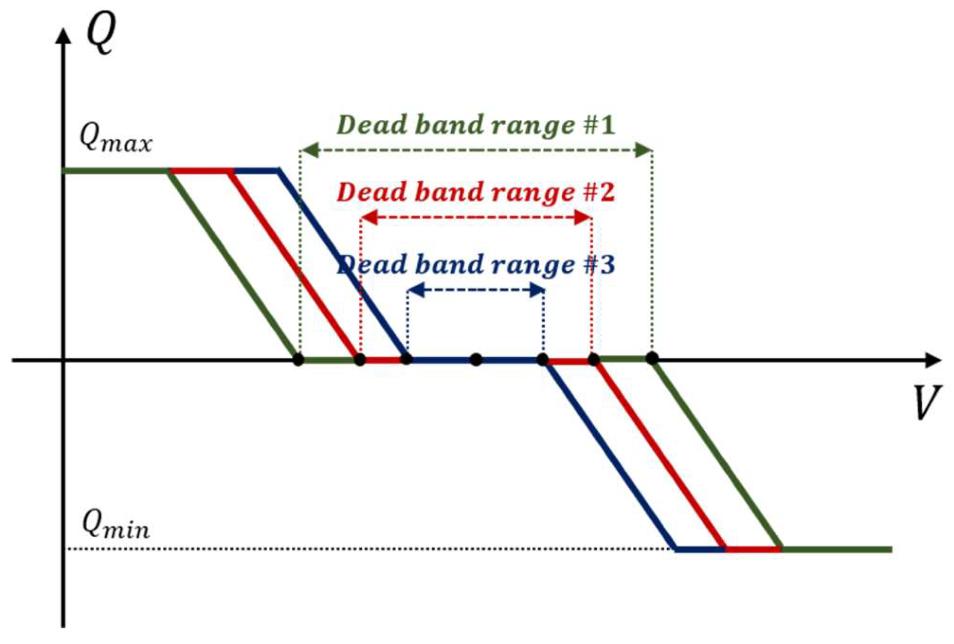
Figure 6.
Flowchart of the proposed scheme including adaptive dead band.
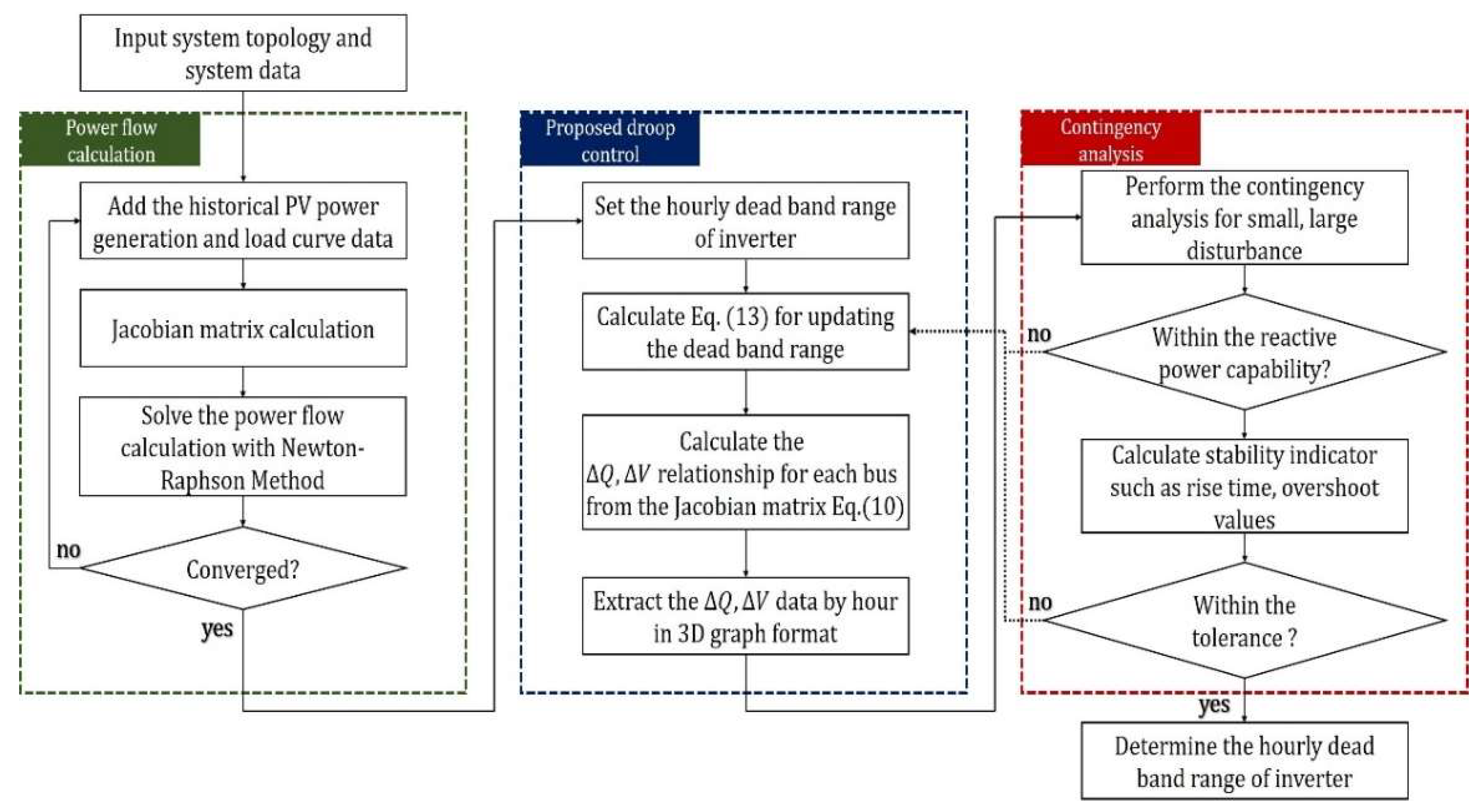
Figure 7.
Modified IEEE 39 bus system diagram.
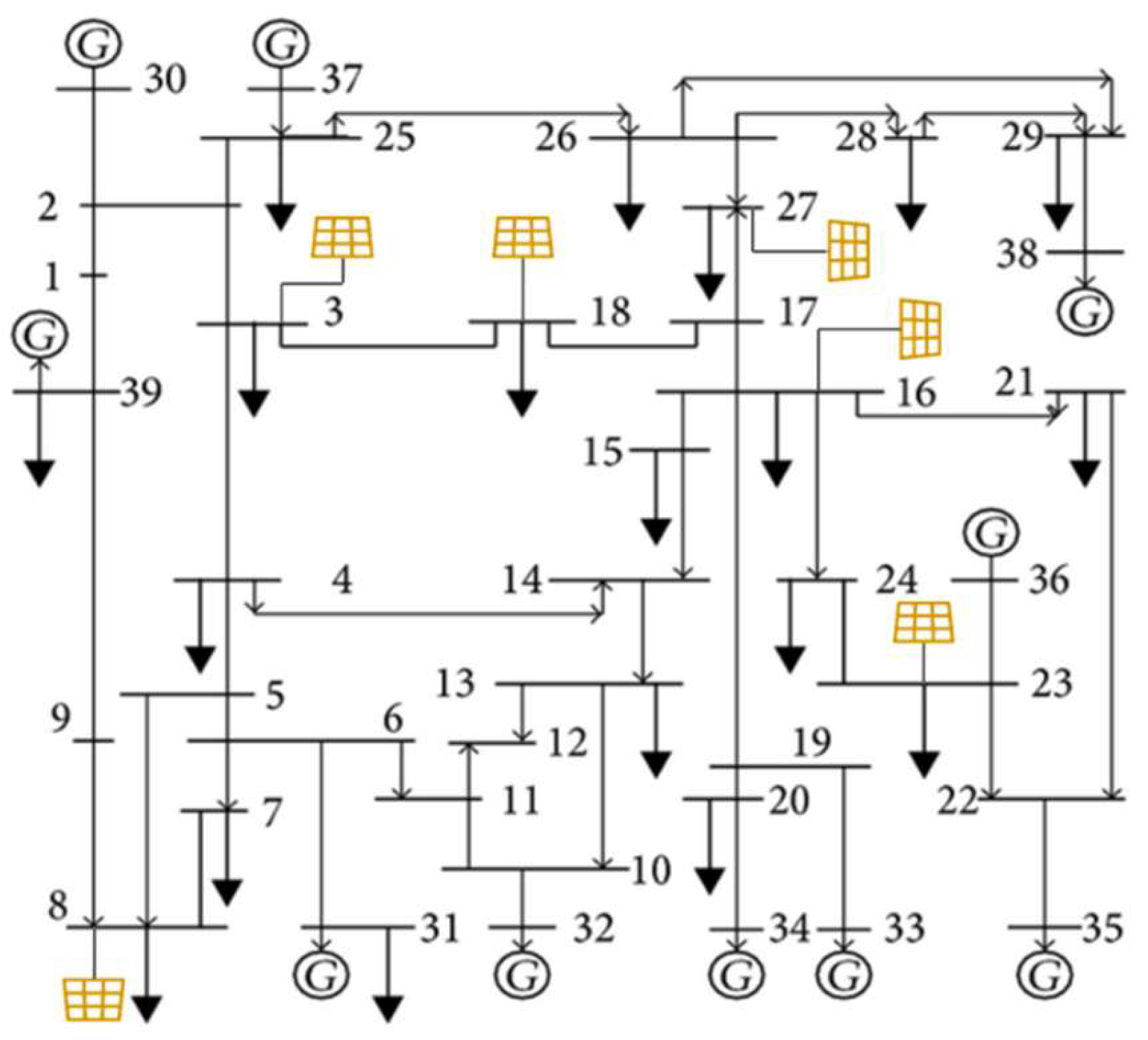
Figure 8.
(a) Boxplot of daily solar generation, and (b) boxplot of daily load curve.
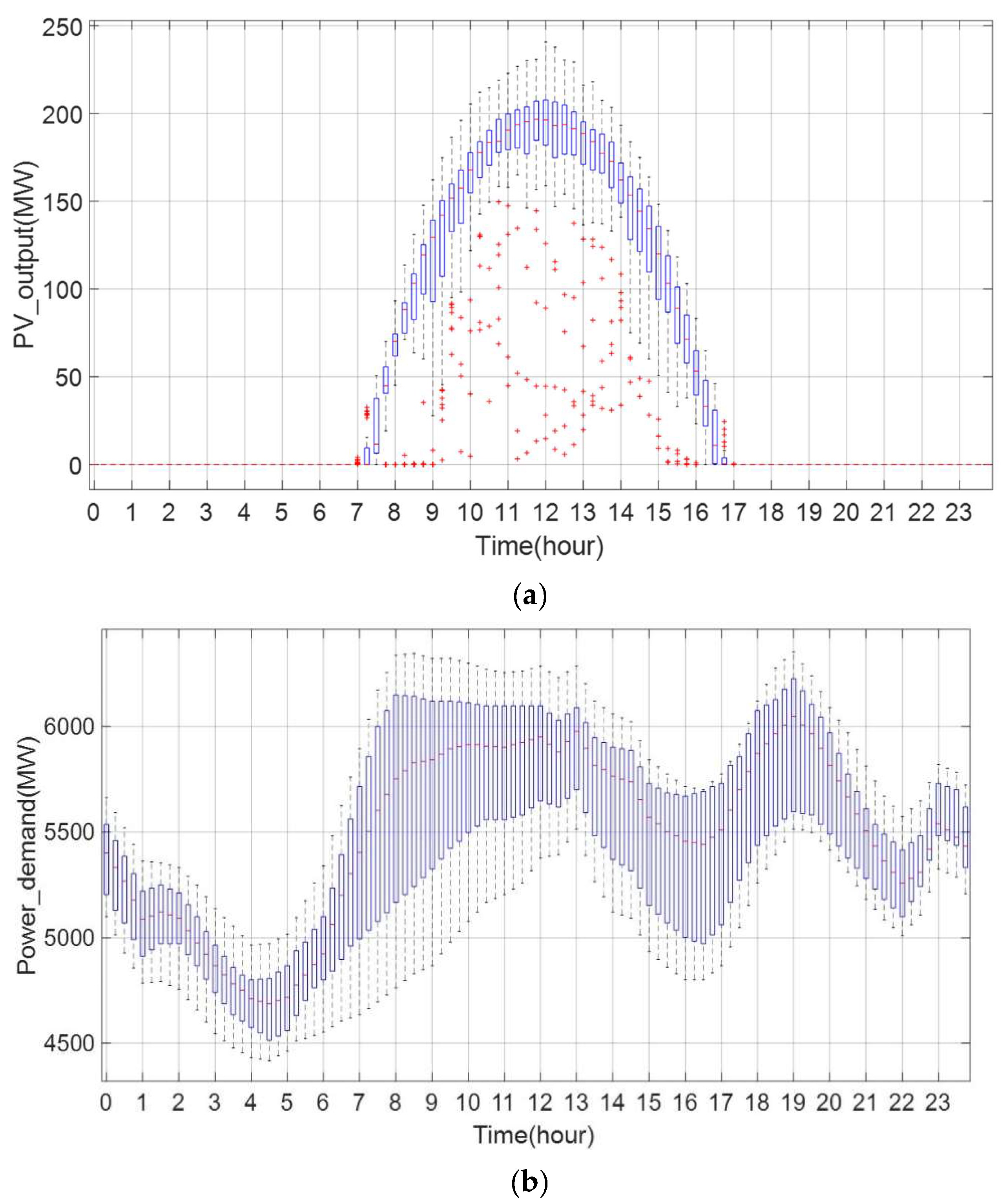
Figure 9.
Voltage profile performance indicator.
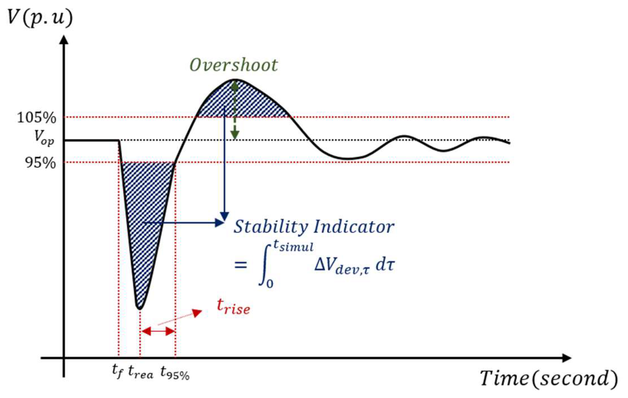
Figure 10.
Performance indicators of the simulation result.
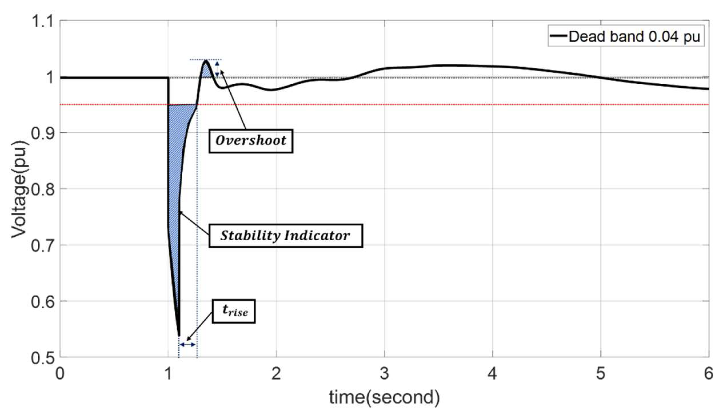
Figure 11.
Voltage profile due to small disturbance.
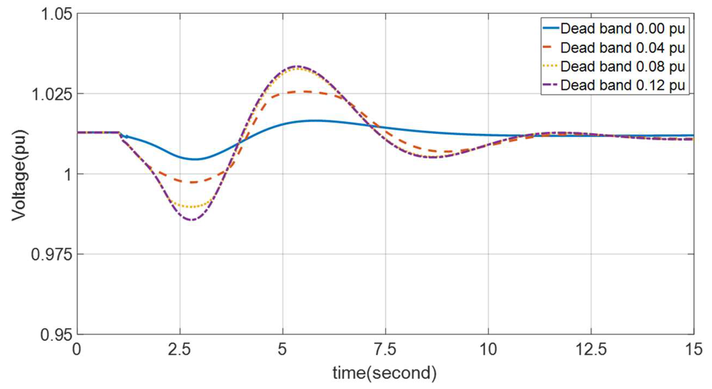
Figure 12.
Voltage profile due to large disturbance.
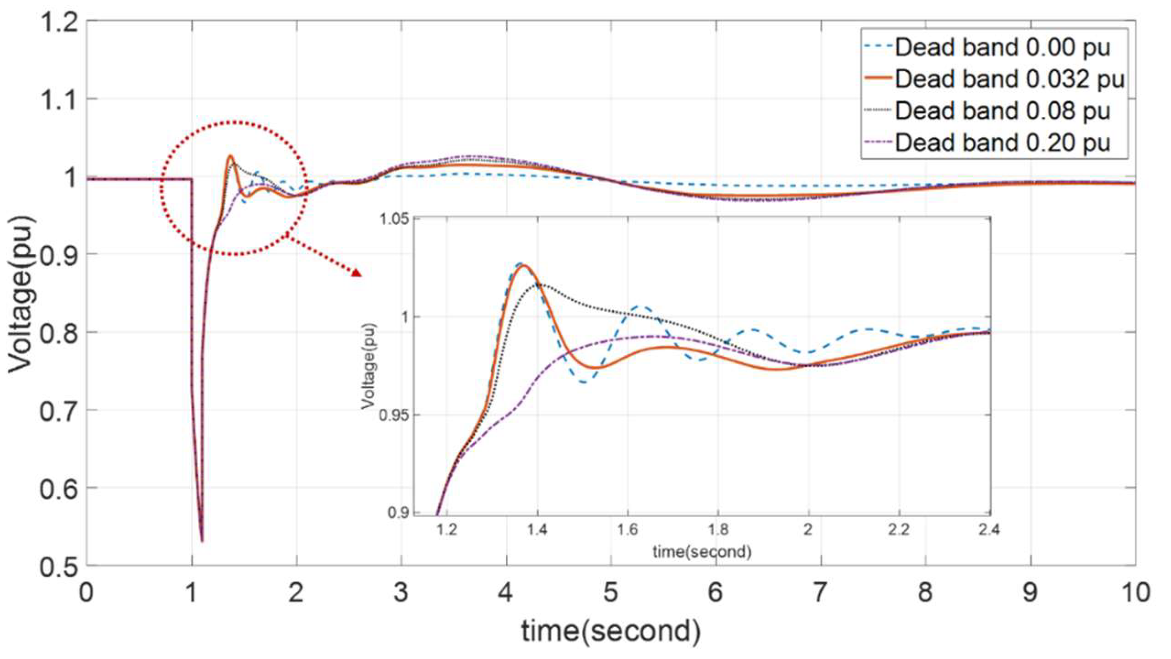
Figure 13.
(a) Voltage profile, and (b) reactive and (c) active power result obtained by large disturbance.
Figure 13.
(a) Voltage profile, and (b) reactive and (c) active power result obtained by large disturbance.
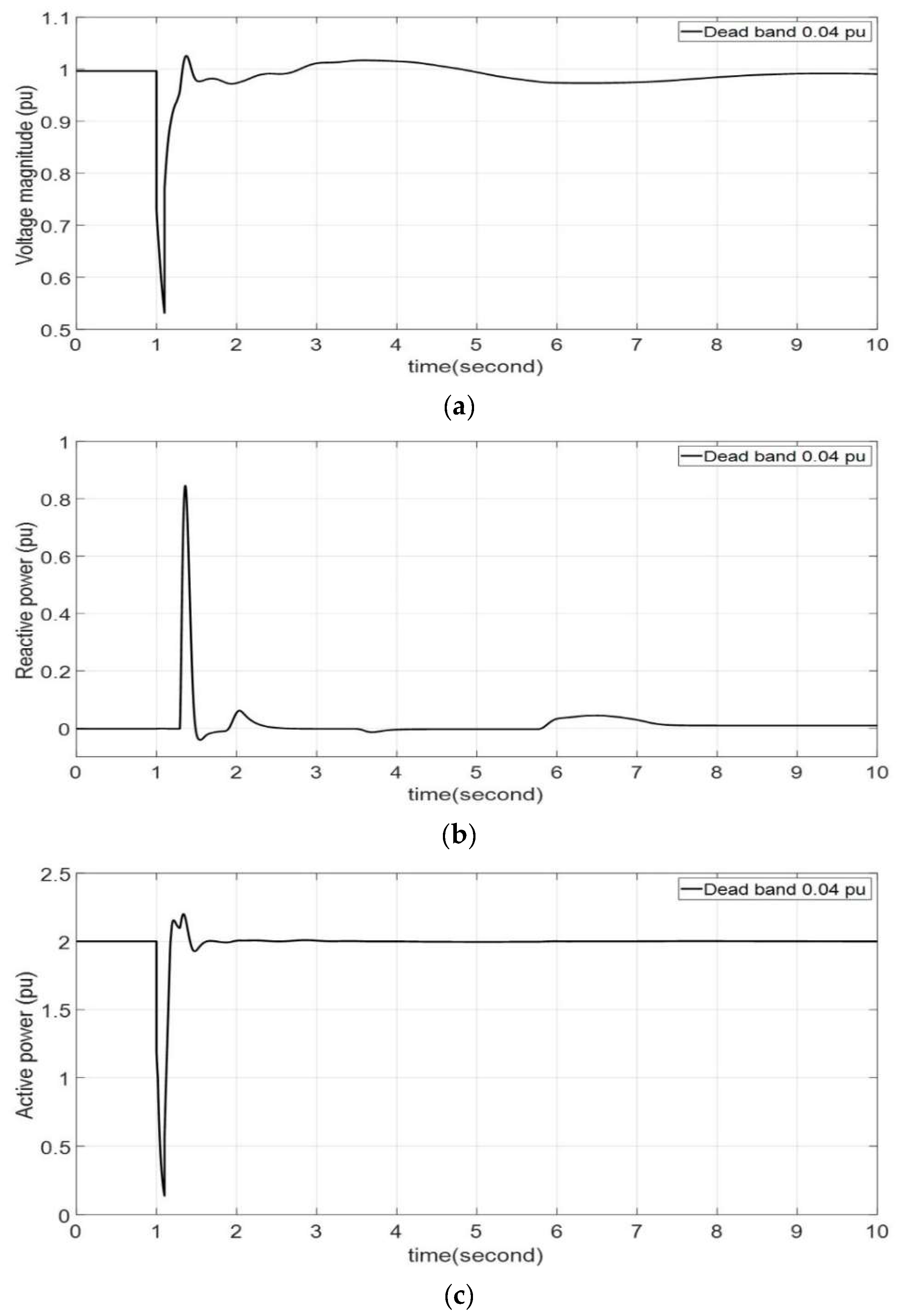
Figure 14.
Net load curve and dead band result by time.


Table 1.
Nomenclature for reactive power-voltage droop control.
| Nomenclature | Description |
|---|---|
| Regulated branch initial reactive power flow (p.u) | |
| Reactive droop (p.u) | |
| Regulated bus voltage (p.u) | |
| Voltage and reactive power filter time constants (s) | |
| Regulated bus initial voltage (p.u) | |
| Maximum Volt/VAR error (p.u) | |
| Minimum Volt/VAR error (p.u) | |
| Volt/VAR regulator proportional gain | |
| Volt/VAR regulator integral gain | |
| Maximum plant reactive power command (p.u) | |
| Minimum plant reactive power command (p.u) | |
| Plant controller Q output lead time constant (s) | |
| Plant controller Q output lag time constant (s) | |
| Reactive power command from plant controller (p.u) |
Table 2.
Performance indicator parameter specification.
| Parameter | Small Disturbance | Large Disturbance |
|---|---|---|
| (s) | <1–30 | <0.2 |
| Overshoot (%) | <5 | <3 |
| Stability Indicator(SI) | <0.0 | <0.05 |
Table 3.
Performance indicators result according to dead band range.
| Parameter | Dead Band (p.u) | ||
|---|---|---|---|
| 0.02 | 0.04 | 0.06 | |
| (s) | 0.161 | 0.162 | 0.163 |
| Overshoot (%) | 3.0909 | 2.9691 | 2.7517 |
| Stability Indicator(SI) | 0.0417 | 0.0417 | 0.0417 |
Table 4.
Performance indicators result according to dead band range.
| Parameter | Dead Band (p.u) | |||
|---|---|---|---|---|
| 0.00 | 0.032 | 0.08 | 0.20 | |
| (s) | 0.177 | 0.179 | 0.185 | 0.235 |
| Overshoot (%) | 3.0985 | 2.9866 | 2.5117 | 2.9359 |
| Stability Indicator(SI) | 0.0437 | 0.0438 | 0.0438 | 0.0440 |
Publisher’s Note: MDPI stays neutral with regard to jurisdictional claims in published maps and institutional affiliations. |
© 2020 by the authors. Licensee MDPI, Basel, Switzerland. This article is an open access article distributed under the terms and conditions of the Creative Commons Attribution (CC BY) license (http://creativecommons.org/licenses/by/4.0/).
Share and Cite
MDPI and ACS Style
Kim, W.; Song, S.; Jang, G. Droop Control Strategy of Utility-Scale Photovoltaic Systems Using Adaptive Dead Band. Appl. Sci. 2020, 10, 8032. https://doi.org/10.3390/app10228032
AMA Style
Kim W, Song S, Jang G. Droop Control Strategy of Utility-Scale Photovoltaic Systems Using Adaptive Dead Band. Applied Sciences. 2020; 10(22):8032. https://doi.org/10.3390/app10228032
Chicago/Turabian StyleKim, Woosung, Sungyoon Song, and Gilsoo Jang. 2020. "Droop Control Strategy of Utility-Scale Photovoltaic Systems Using Adaptive Dead Band" Applied Sciences 10, no. 22: 8032. https://doi.org/10.3390/app10228032
Note that from the first issue of 2016, this journal uses article numbers instead of page numbers. See further details here.