Improvement of Electric Propulsion System Model for Performance Analysis of Large-Size Multicopter UAVs


1
Department of Aerospace Engineering, Pusan National University, Busan 46241, Korea
2
Korea Electrotechnology Research Institue, Changwon 51543, Korea
*
Author to whom correspondence should be addressed.
Appl. Sci. 2020, 10(22), 8080; https://doi.org/10.3390/app10228080
Submission received: 21 September 2020
/
Revised: 31 October 2020
/
Accepted: 12 November 2020
/
Published: 15 November 2020
(This article belongs to the Special Issue Aerospace System Analysis and Optimization)
Abstract
:In this study, an improved model of the electric propulsion system is proposed in order to analyze the performance of large-size multicopter unmanned aerial vehicles. The main improvement of the proposed model is to reflect the armature reaction of the motor, which effectively explains the significant performance degradation in high-power operation. The armature reaction is a phenomenon, in which the main field flux is interfered by a magnetic flux and, as the size and output of the motor increase, the effect of armature reaction also rapidly increases. Therefore, the armature reaction must be considered for the optimal design and performance analysis of large-size multicopter platforms. The model proposed in this study includes several mathematical models for propellers, motors, electric speed controllers, and batteries, which are key components of the electric propulsion system, and they can calculate key performance data, such as thrust and torque and power consumption, according to given product specifications and input conditions. However, estimates of the armature reaction constants and heat profiles of motors need to be obtained in advance through experimental methods, since there is not yet enough data available in order to derive an estimation model. In conclusion, a comparison with the static thrust test of some commercial products confirmed that the proposed model could predict performance in the high-power operation of electric propulsion systems for large multicopter platforms, although some errors were noted.
1. Introduction
Currently, large-size industrial multicopter platforms with payloads of several tens of kilograms or more are being developed. These large platforms aim to load special heavy payloads, such as large-capacity cargo transport, fire-fighting equipment, first-aid equipment, and military supplies. Such platforms are expected to further expand the scope of the aviation industry, because they can overcome challenges that cannot be overcome by conventional small aircraft or drones. Furthermore, the basic shape of an urban air mobility (UAM), which have attracted attention as next-generation transportation vehicles, is often based on the multicopter platform. The Passenger AAV (Ehang-216) of Ehang, the Volocity of the Volocopter, and the CityAirbus of the Airbus are typical cases of multicopter-type UAMs [1,2,3].
Meanwhile, as the size of the platform increases, factors that are to be considered in the design process also increase and become challenging. In terms of the structural strength of the platform, the scale effect of material stiffness, which could have been a benefit in small sizes, is reduced [4]. Thus, more complex structural designs than those of small platforms are required. The high risk of failure and crash, which increases in proportion to the platform weight, is another challenge. For example, in the case of small multicopter unmanned aerial vehicles (UAV), emergency parachutes against falls or propeller guards against collisions are included in the recommendation, but not necessarily used. In contrast, for large-size platforms, these features are strongly demanded as essential design requirements to ensure safety. However, these requirements often result in an increase in weight, which, in turn, leads to reduced power efficiency across the platform. As is well known, a short flight time due to low power efficiency is the main weakness of multicopter platforms.
In this regard, research on the optimal design of multicopter platforms is being conducted in various fields. The development of reliable models for performance analysis of electric propulsion systems is one such effort. The propulsion system model forms the basis for reviewing the overall performance of the platform and performing the optimal design; thus, the development of a reliable model is usually a priority for the aircraft design process.
For large-size multicopter UAVs, it must be considered that the system will operate under high voltage and heavy current conditions as the size of the electric propulsion system increases. Especially in these high power conditions, the effect of the motor’s armature reaction is no longer negligible. The armature reaction is a phenomenon, in which the main field flux is interfered by a magnetic flux that is caused by current flowing through the armature of the motor and it is known to be the main cause of stray losses [5].
In this study, as part of the development of optimal design tools for large-size multicopter UAVs, research on the improvement of a multidisciplinary model of an electric propulsion system was performed. It was focused on improving the reliability of the model for electric propulsion system, and supplementing the dynamics and statistical analysis for each component based on the previous studies [6]. In particular, for motor models, the degradation of rotor performance under high-power conditions can be more accurately predicted by modeling the effect of the armature reaction. A simple thermal effect model was also added to describe the degradation of performance due to overheating of the motor. For statistical analysis, the overall analysis of commercial products dedicated to multicopter UAVs was conducted. Based on this, replaceable models were presented for some factors that were treated as constants or were neglected in previous studies, such as no-load current of motors or power losses in electric speed controllers (ESC). The developed performance analysis model basically reflects only static operating conditions and, therefore, does not take into account the transient characteristics, such as due to a disturbance in flight; however, it is constructed to suit the iterative calculation for initial sizing or optimal design based on simple equations. Finally, the developed model was verified by comparison with data sheets and static thrust test results for actual commercial products. Validation has confirmed that the performance analysis of the electric propulsion system for large-size multicopter UAVs can be more reliably performed through major improvements, including the armature reaction model. However, in order to use the proposed model, a preliminary experiment for each motor product is still needed in order to estimate the armature reaction constant and thermal profile; thus, follow-up research is underway to secure the estimated model.
2. Related Works
Recent research on performance analysis and optimal design methods for multicopter UAVs has been earnest. Initially, studies on small electric-powered fixed-wing UAVs mainly focused on performance analysis and modeling methods for multicopter platforms, owing to their similar configurations.
Lundström et al. [7] analyzed the modeling of a simple propulsion system consisting of a single motor and a propeller for the design automation of flying wing micro aerial vehicles (MAV). The study shows a typical form of the electric propulsion system model for small UAVs; however, the reliability of the model is not very high, because the dynamics could not sufficiently explain the behavior of the components.
Gur et al. [8] performed an optimization study of an electric propulsion system for small fixed-wing UAVs. For multicopter platforms, Bershadsky et al. [9] conducted similar studies. Both of the studies presented a multidisciplinary design optimization (MDO) framework for the initial sizing process based on statistical analysis and dynamics of the key performance variables of each component of the electric propulsion system. The two studies highlighted the same problem of low reliability of some statistical data. This is because the sample population for statistics targeted overly generic products, and the correlation between some variables was incorrectly analyzed. In the case of Bershadsky et al., this problem might have been inevitable at the time of the study, because there were not enough commercially available multicopter UAVs.
Gong et al. [10,11,12] presented a more detailed model for fixed-wing aircrafts and demonstrated that the accuracy of the model can be effectively improved by focusing on the detailed characteristics of each component of the electric propulsion system.
One recent notable study is the Conceptual Layout Optimization for Universal Drone Systems (CLOUDS), a multicopter performance analysis and conceptual design program that was developed by Seoul National University through a joint study with the Korea Aerospace Research Institute [13,14]. CLOUDS provides performance analysis and conceptual design tools for small multicopter platforms weighing 25 kg or less, based on the blade element momentum theory (BEMT) and electric propulsion system model.
However, most of the above studies were conducted on small UAVs and did not include factors that should be considered in the high-power operation of large motors, such as armature reaction or thermal effects. Thus, errors are common when comparing the model results with performance data or experimental results in high-power operations.
3. Electric Propulsion System for Multicopter UAVs
A multicopter is a rotorcraft that has more than two lift-generating rotors. The most prominent feature of the multicopter that distinguishes it from conventional helicopters is its simple configuration. Instead of a large rotor blade and complex hub structures, it simply uses multiple propellers that were directly connected to the motors. Figure 1 shows the typical configuration of the electric propulsion system for multicopter UAVs, which consist of multiple motors and propellers, ESCs, and batteries.
Each rotor on a multicopter platform typically includes components with the same specifications. For the motor type, a permanent magnet outer rotation brushless direct current (BLDC) motor with a large number of poles is preferred. During operation, the output of the motor moves along the torque-to-speed curve of the propeller. For propellers, a two-blade fixed pitch propeller type that is made of carbon fiber reinforced composite material is preferred. Usually, one rotor arm has one propeller; however, some platforms are equipped with two propellers, each coaxially inverted to reduce the overall size. The ESC refers to a motor driver and it controls the output level of the motor by regulating the input voltage. Although the ESC is conventionally called a speed controller, it does not actually quantitatively control the speed of the motor. For type of batteries, lithium-based secondary batteries are commonly used. In this study, only models for lithium-polymer (LiPo) batteries were considered.
4. Mathematical Model
Similar to the actual system, the model for the electric propulsion system includes subgroups for each of the four components. Each subgroup consists of simple models that are based on multidisciplinary dynamics and parameters of the electric propulsion system, and it has been modeled to reflect as many factors that significantly affect the performance of the platform as possible.
4.1. System Power Chain
Figure 2 shows the system power chain, illustrating the power transfer structure of the typical multicopter UAV [15]. The flight control system (FCS) includes both avionics and additional servo actuators for flight control. Usually, the avionics of the multicopter UAV is simply configured with a flight control computer, navigtation sensors, and telemetry modems. The payload includes all of the additional equipment for missions. In the case of multicopter UAVs, typical payloads are cameras and gimbals for the aerial photography, LiDAR sensor for airborne laser scanning, and devices for transporting special cargo.
The total power consumption () of the multicopter UAV is calculated, as shown in Equation (1), where is the power usage of the UAV system and is the power loss of the battery. The power usage of the system is divided into the required rotor power () and the power consumption in the FCS and payload (, ), as shown in Equation (2). The required rotor power is the sum of the power consumed by the motor () and the ESC loss (). The calculation of the required rotor power is defined as Equation (3), where is the number of rotors. Assuming that the output of all rotors is constant and stable under steady state flight, such as hovering or cruise flight conditions, Equation (3) can be simplified as Equation (4). The power that is consumed by the FCS and payload is considered to be constant.
4.2. Propeller
In this paper, the propeller model was written as a regression model based on the static thrust test data of the sample propeller used in the actual experiment in order to minimize the error of the propeller model for effective verification of proposed electric propulsion system model. The propeller model comprises formulas for thrust and torque calculation and submodels for thrust and torque coefficients. In this study, the thrust and torque coefficient model was developed as a regression model based on the momentum theory and actual performance test, and only the static thrust condition was considered. This was done in order to validate the proposed electric propulsion system model as correctly as possible and it is based on the static thrust data that were obtained from the actual experiment for commercial propeller samples.
According to the standard definition of propeller aerodynamic coefficients, the propeller thrust and torque can be calculated using Equations (5) and (6) [16], where and are the propeller thrust and torque, respectively; and are the thrust and torque coefficients, respectively; is the air density; n is the propeller speed in revolutions per second; and, D is the diameter of the propeller.
The aerodynamic coefficient of the propeller is expressed as a function of geometrical features, Reynolds number, tip speed, and advance ratio. The geometrical features can be represented as the diameter of the propeller and the pitch ratio. The Reynolds number and tip speed are determined while using the diameter and speed of the propeller, and the advance ratio is not considered in the static thrust condition. Thus, the aerodynamic coefficients of the propeller under static thrust conditions are modeled as a function of diameter, rotational speed, and pitch ratio, as shown in Equation (7), in which and are the static thrust and static torque coefficients, respectively; and, k, a, b, c are the coefficients of the regression model.
4.3. Motor
The motor model is based on the direct current (DC) motor fundamentals and simple electrical model [5]. Figure 3 depicts the equivalent circuit of the simple DC motor model, where the propeller torque acts as a load, and the basic equations are as shown in Equation (8) and (9). Where is the applied voltage; and are the motor inductance and resistance, respectively; is the current consumption; is the back electro motive force (EMF); is the voltage drop due to an armature reaction; is motor torque; is motor speed in radian per second; and, is the viscous friction coefficient. Although the construction of the model is simple, it contains all of the basic electrical and mechanical elements required in order to represent motor dynamics. This is appropriate when it is necessary to examine the overall behavior characteristics as simple as possible with adequate fidelity, as in this study.
Equations (8) and (9), respectively, reflect the electrical and mechanical characteristics of the motor, and, if there is no change in speed of the motor, the differential terms are eliminable as Equations (10) and (11). The input and output power of the motor are calculated while using Equations (12) and (13), and the efficiency is calculated using Equation (14).
The relationship between mechanical energy and electrical energy can be expressed using motor constants. Equations (15) and (16) show that the back EMF and motor speed, motor torque, and current consumption are linearly proportional, where is a back EMF constant and is a torque constant. The mechanical power output of the motor and the power by back EMF have the same values, according to the law of energy conservation. This can be expressed as Equation (17), and applying the Equations (15) and (16) here, it can show that the motor torque constant and the back EMF constant also have the same value. The speed constant, , which is provided as a key performance index from most multicopter motor manufacturers, represents the motor speed per unit voltage in the no-load condition (), as shown in Equation (18). This corresponds to the inverse of the back EMF constant. Thus, each motor constant is combined as one, as in Equation (19).
A motor size constant, , another important reference index when selecting a motor, is expressed as the ratio of the motor torque and the square root of resistive power loss and it can be calculated from the torque constant and the motor resistance, as Equation (20). The motor size constant is proportional to the weight of the motor and it is also useful for estimating the viscous friction coefficient. This is because the viscous friction coefficient also tends to be proportional to the size of the motor. Although the viscous friction coefficient is not usually provided as a product specification of the motor, the value can be estimated from the no-load current. From the Equation (11), if there is no external load, the viscous friction can be regarded as the only load applied to the motor. The estimation equation for viscous friction coefficient is as shown in Equation (21) and it is derived from Equations (11), (16), and (18). Where is a no-load current and is an applied voltage under no-load current measurement conditions. These values are usually given in the specification of the motor. Figure 4 shows a tendency of the viscous friction coefficient relative to the motor size constant. Data for this trend analysis were obtained based on the product specifications of the major motor manufacturers for multicopter UAV [17,18,19,20]. Consequently, the estimated model for the viscous friction coefficient of the BLDC motor for multicopter UAVs was obtained, as shown in Equation (22).
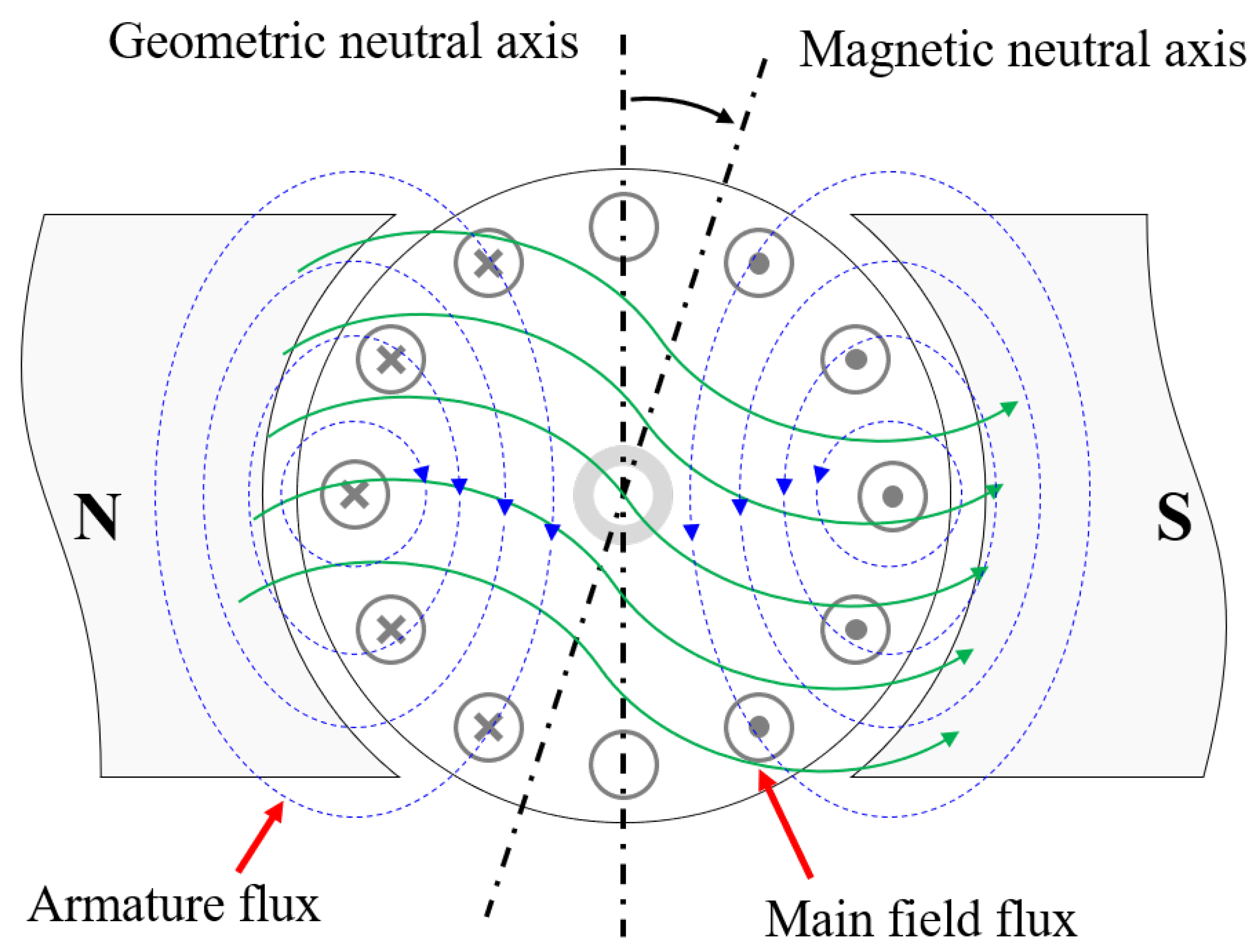
On the otherhand, during actual operation, the performance of the motor is affected by a number of factors. Among the various factors that degrade performance, the most representative is an armature reaction. Figure 5 is a simple diagram of the typical armature reaction of a two-pole DC motor, showing that the main field flux is affected by the armature flux, which results in an magnetic neutral line being misaligned from a geometric neutral line [21].
In the case of motors for general industrial machinery, where the operation range is usually set as the design value and does not deviate much from that the design value, this is offset by installing compensation winding in order to match the expected level of the armature reaction. Thus, in many cases, the effect of the armature reaction is often considered to be negligible. However, in motors for multicopter UAVs, notably, almost all products are not designed with consideration for the armature reaction. This is because motors for multicopter unmanned aerial vehicles are driven by speed control methods, which makes it difficult to reflect specific points, such as design values, owing to their wide operating range. In addition, because aircraft parts are sensitive to weight, the motor is designed to be as light and simple as possible; therefore, the installation of compensation winding is difficult.
In addition, the effects of armature reactions are particularly noticeable in high-power conditions; thus, the larger the platform and motor size, the more necessary it is to consider armature reactions more carefully. In motors that ere used in small multicopter platforms, the effect of the armature reaction is usually observed in the short range near full throttle conditions. In contrast, in large-sized motors where a high-voltage, high-current drive is based, it can be seen that the armature reaction is prominent in the wide range starting from the intermediate throttle. However, because armature reactions are influenced by complex factors, such as stator shape and air gap, number of winding turns in coils, and magnetic flux in magnets, the analytical model for armature reactions is also very complex and difficult to express explicitly [22]. Thus, the armature reaction is usually considered to be simplified into additional voltage drop factors, as is included in Equation (8). According to the related studies that are referenced in this paper, it is mainly expressed as the product of the n-order polynomial for the motor current and the motor speed [23,24,25]. In conclusion, in this study, a function of the squared motor current and the motor speed was used as the model, such as Equation (23). Where is the armature reaction constant, which can be used to estimate the appropriate value through comparison with the experimental data. Although this is a more simplified expression when compared to the forms presented in the referenced studies, given the weight of each order term according to the coefficients of the polynomials that are presented in those studies, it was considered to be sufficient for the level of the model that is required for this study.
Meanwhile, the thermal effects on the motor reduce the magnetic flux density and cause increased winding resistance [26,27,28]. This is not as high as that caused by an armature reaction; however, it can also cause significant degradation if excessive overheating occurs. Indeed, the demagnetization of the magnet and the increase in the internal resistance of the motor due to the thermal effect cause a sharp increase in the current consumption. The change in magnetic flux density is directly related to the torque constant and back EMF constant of the motor, which can be expressed while using a temperature coefficient. Equation (24) can be used in order to calculate the change in torque constant and back EMF constant due to thermal effects, where is the temperature coefficient of the conductor; is the temperature change of the magnet; and, subscript ‘o’ represents ordinary conditions. Similarly, the change in motor resistance is calculated, as shown in Equation (25), where is the conductor temperature coefficient of the motor coil and is the temperature change of the conductor.
Table 1 lists the average temperature coefficient and the temperature limit for each type of magnet. Temperature limits are the maximum temperatures at which a magnet can maintain a minimum magnetism, which is a decisive factor in the operating limits of the motor. Most BLDC motors for multicopter UAVs are equipped with N42 or N45 grade neodymium (NdFeB) magnets. Therefore, it is recommended that these magnets not be overheated to more than 100 °C during operation. Table 2 lists the temperature coefficients of typical conductor materials, mainly copper and silver wires used in motor coils.
4.4. ESC
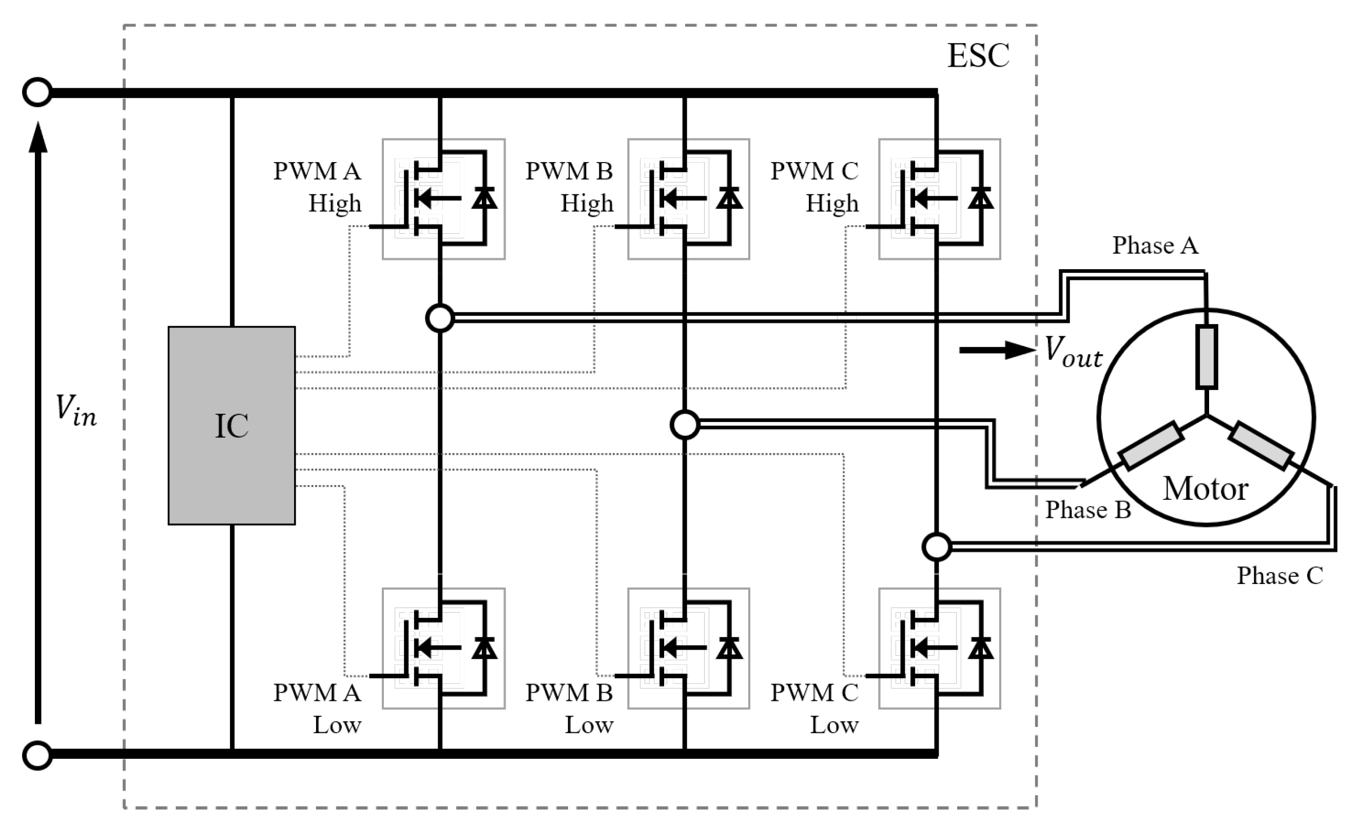
The ESC uses switching circuits that consist of multiple metal oxide semiconductor field-effect transistors (MOSFET) to convert DC electricity from the power source into a three-phase waveform for motor control [29,30]. There are two typical control methods for motors for multicopter UAVs: trapezoidal commutation and field oriented control(FOC). The conventionally used method is trapezoidal commutation. The switching circuit consists of at least six MOSFETs depending on the ESC capacity, as shown in Figure 6. The three-phase waveform is controlled by switching the high and low side MOSFETs, and the applied voltage to the motor is regulated from the input voltage by pulse width modulation (PWM). This results in a conduction loss and a switching loss due to the on/off operation of the MOSFET, which are the main power loss factors for the ESC.
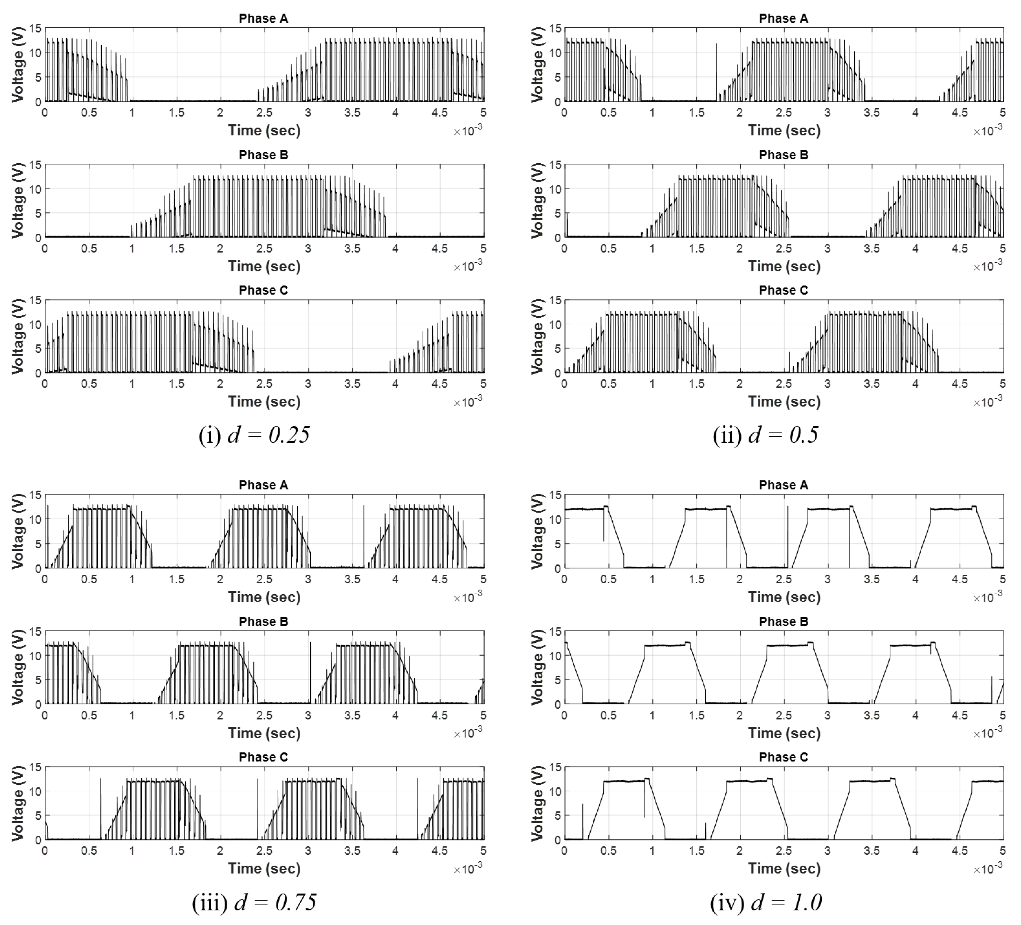
Figure 7 shows PWM signal waveforms for high and low side MOSFET control and three phase voltages in the ideal trapezoidal commutation. Figure 8 shows actual three phase voltage waveforms according to the PWM duty ratio (d) of the output voltage, which was measured by an experiment driving the actual motor(T-motor U5 motor with Flame 40A ESC, 3S1P LiPo battery) under the no-load condition. As the PWM duty ratio increases, it shows that the width of the pulse that forms the phase voltage waveform, which may seem like noise, is widening. Finally, when the PWM duty ratio reaches 1, it shows that the traces of pulse disappear from the phase voltage and only the phase transition of the neat trapezoidal waveform takes place. For most multicopter dedicated ESCs, the PWM duty ratio directly refers to the motor throttle command from the flight controller. On the other hand, the shorter cycle of trapezoidal waveforms that are inversely proportional to the PWM duty ratio is due to the increased commutation frequency as the motor speed increases. Consequently, the value of the output voltage (), which is the time average of the actually applied voltage to the motor, can be calculated, as shown in Equation (26).
The total power consumption of the ESC can be approximated by the sum of the conduction loss (), switching loss (), and integrated circuit (IC) operating power(), as shown in Equation (27) [11,31,32,33,34].
The conduction loss of the MOSFET is calculated from the output current and on-state resistance. For the ESC, the output current is the current consumption of the motor. To obtain the total conduction loss of the ESC, the number of MOSFETs in the on-state must be considered according to the commutation sequence and PWM duty ratio that determines the time of the on-state. Thus, the total conduction loss is calculated, as shown in Equation (28), where is the ESC total on-state resistance.
The switching loss is due to a gate charge of the MOSFET. The gate charge is the amount of charge that needs to be injected into the gate electrode to turn on the MOSFET completely. While the gate of the MOSFET is fully open, the power on the MOSFET will be lost as much as the gate charge is charged. Conversely, while the gate of the MOSFET is closed, the loss is caused by the gate that is not fully closed until the gate charge is completely discharged. Here, the time that is required to charge and discharge the gate charge it is called the rise and fall time, which depends on the structural and material characteristics of the MOSFET. Power MOSFETs for high-speed switching typically have a rise and fall time in the tens of nanoseconds. The input voltage of the ESC is adjusted to the applied voltage via the high frequency PWM, as shown in Figure 8. The time that is required for the gate of MOSFET to open and close is actually extremely short, but the total amount cannot be ignored if the MOSFET operates at a very high frequency, like ESCs. Switching loss of the ESC can be computed while using Equation (29), where and are the rise time and fall time of the MOSFET, respectively; and, is the terminal voltage of the battery pack as the input voltage on the ESC. is the switching frequency, which varies depending on the ESC product and settings, and it is commonly 8 kHz, 16 kHz, and 32 kHz. In this study, 16 kHz was used as the default value.
The model of on-state resistance and the default rise/fall time were derived based on typical values on the rated condition given in the datasheets for MOSFET chips. To this end, some major commercial ESC products have been investigated and analyzed. Table 3 lists the specifications for sample commercial multicopter-dedicated ESCs and the MOSFETs used in these products [17,35,36,37]. Note that, for the data on the MOSFET, because of that datasheets for the ESC did not provide any relevant information, it was obtained by disassembled the actual sample ESC products. Additionally, the detailed specifications of the MOSFETs were referenced from the specifications for each of the chips.
Figure 9 shows the relationship between the allowable maximum continuous current and on-state resistance, arranged from the specifications of the sample ESCs outlined in Table 3, and the estimation model is shown in Equation (30). Where is the current-carrying capacity of the ESC, similar to the maximum continuous current on the datasheet. The current consumption of the motor under the full throttle condition should be less than the maximum continuous current of the ESC.
For MOSFETs applied to the sample ESCs, as shown in Table 3, the sum of the rise and fall times is up to 87 nSec and at least 8.9 nSec. However, this shows a trend that has no relationship with any specifications of the ESC. Therefore, in this study, 30 nSec—the average of the MOSFETs used in the sample ESCs—was used as a default value for the sum of rise and fall times. Similarly, the ESC IC operating power was considered to be constant at 0.5 W, which was obtained by referring to the datasheet of some sample products.
4.5. Battery
The main challenge with the battery model is describing the voltage drop due to internal resistance. Assuming that the effects of the disturbance in flight are small enough to be neglected and that the output of all motors remains stable, the drain on the battery can also be seen as a constant steady discharge. In this paper, the battery model refers to a simple model with only one internal resistance, as shown in Figure 10.
The terminal voltage, , of the battery is calculated, as shown in Equation (31), where is the open-circuit voltage of the battery, is the load current, and is the internal resistance of the battery. The load current is the total current consumption of the entire UAV system, as shown in Equation (32). From Equations (31) and (32), the equation for the terminal voltage is derived, as shown in Equation (33). The open-circuit voltage of the LiPo battery depends on the state of charge () and outputs per cell of approximately 4.2 V in the fully charged condition and approximately 3.4 V in the fully discharged condition. The nominal voltage is based on the open-circuit voltage of the half-charged condition (), which is approximately 3.7 V per cell. The energy capacity of the battery is given by multiplying the electric charge capacity by the nominal voltage, and the total energy capacity is calculated, as shown in Equation (34).
The LiPo battery comprises a series/parallel connection of multiple single cells, as illustrated in Figure 1. Thus, the total internal resistance of the battery set () can be calculated while using Equation (35), where is the number of serial-connected cells that are contained in a single battery pack, and is the number of battery packs connected in parallel. The internal resistance of a single LiPo battery cell () depends on the electric charge capacity.
In this study, experiments were conducted on single-cell LiPo battery samples that are shown in Figure 11 in order to obtain estimation models of the battery open-circuit voltage and the internal resistance according to SoC. The maximum discharge rate of the sample cells that are mainly used in multicopter UAVs is approximately 25 C.
Figure 12 shows the average tendency of open circuit voltages according to SoC measured in a discharge experiment on single cell LiPo battery samples. Equation (36) shows the model estimated from the hysteresis curve.
The measurements for the internal resistance were performed while using a DC load method relative to the nominal voltage at room temperature (24 C). Other major factors that affect the change in internal resistance are the operating temperature of the battery, the deterioration of performance due to aging, and theSoC; however, only the normal condition was considered in this study. Figure 13 shows the tendency of internal resistance of the sample battery cells to the capacity. Equation (37) shows the model of the internal resistance estimated from this tendency.
5. Model Implementation
For model implementation, OpenMDAO, an open-source MDO framework provided by NASA’s Glenn Research Center, was employed [38]. OpenMDAO is based on Python language and it provides useful libraries and features that include various solvers and drivers for system analysis or the multidisciplinary optimal design problem. This makes it relatively easy to perform system analysis and optimization problems, even if users are not familiar with mathematical methods.
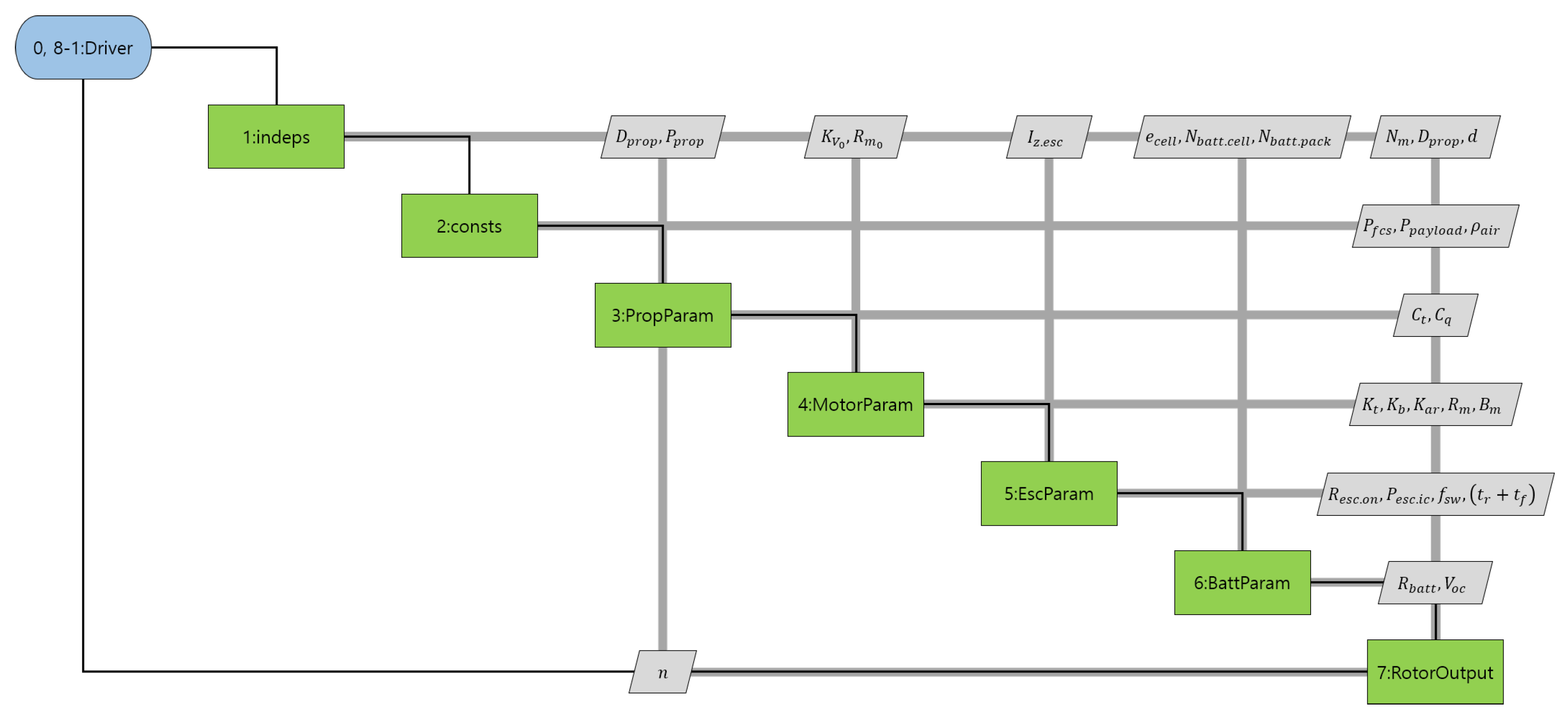
Figure 14 shows an expanded design structure matrix (XDSM), which summarizes the performance calculation process of an electric propulsion system, and has automatically generated using the OpenMDAO visualization feature plug-in [39,40]. Here, “1:indeps” denotes a group of independent variables that correspond to the design variables in the design problem of the electric propulsion system, such as propeller diameter, pitch, and motor specifications. Similarly, “2:consts” denotes a group of components that are treated as constants, such as air density, power consumption in the flight control system, and payload. Groups 3 to 6 are submodels that contain the relevant constants and parameter calculations of each component of the electric propulsion system, and finally, “7:RotorOutput” calculates the various conditions and results of rotor operation.
Figure 15 is a diagram that depicts the configuration of the entire model in more detail. The same with the XDSM, the diagram was also automatically written through the visualization feature of OpenMDAO. From the list of groups and components name on the left, the N2 diagram provides a more detailed view of the group configuration that was simply illustrated in the XDSM. For the electromotive system model implemented in this paper, all of the components, except independent variables or constants, are declared to be explicit components. Explicit components include a formula for that variable, and the various models that are presented in Section 4 are written here. Additionally, as shown in the lower triangular matrix on the diagram, this problem includes cycles for calculations of the propeller thrust and torque, the armature reaction of the motor, and the voltage drop of the battery. Solvers applied for the problem were DirectSolver and Block Gauss–Seidel NonlinearSolver with Aiteken Relaxation [41].
6. Model Validation
In order to validate the proposed model, performance data, static thrust test data, and performance prediction results using the proposed model of several commercial products were compared. Table 4 summarizes the specifications of the sample sets used for validation, with products from T-motor and KDE Direct providing relatively detailed data [42,43,44]. For power sources, a 12,000 W capacity power supply was used for the experiment and, for performance analysis, a LiPo battery model (12S1P 18,000 mAh capacity) was used. Here, the capacity of the battery model was set to have an internal resistance similar to the estimated internal resistance of the power supply from the voltage drop tendency of the static thrust test results.
6.1. Experiment
6.1.1. Method
The static thrust test was performed while using a thrust stand (RCbenchmark Series 1780 [45]) obtained from the Korea Electrotechnology Research Institute. Figure 16a shows the actual configuration of the thrust stand. All of the experiments were conducted in an indoor test environment under normal atmospheric conditions of approximately 25 °C, and the thrust stand was calibrated using a dedicated tool before each experiment. Figure 16b shows a diagram of the data acquisition structure of the static thrust test. During the experiment, a separate thermal imaging camera (FLIR-T62101) was used in order to track the temperature change of the motor. Figure 17 shows the actual thermal images which taken during the test for sample set 2. In order to determine the difference between the temperature of the stator inside the motor and the temperature of the external rotor, each measurement was taken separately.
6.1.2. Result
Figure 18, Figure 19 and Figure 20 illustrate the comparisons of the experimental results for three sample sets with the performance data that were provided by the manufacturer. Notably, the terminal voltage of the datasheet was estimated by dividing the input power by the current consumption, because it was not provided in the performance data. For KDE Direct products, no values are provided for the propeller torque either. In contrast, KDE Direct provides performance data based on lithium high-voltage batteries and not LiPo batteries. However, the applied voltage was fixed at 50 V in the experiments, owing to problems that are associated with equipment setup. Therefore, the experimental results were indirectly compared with data of similar applied voltages in the datasheet.
In sample set 1, the rotational speed, as shown in Figure 18c, shows a tendency that is relatively consistent with the datasheet. However, the thrust and torque that were produced at the same rotational speed were quite low. For the terminal voltage, as shown in Figure 18d, the measured value shows an obvious drop as the motor output increases, whereas the estimated voltage on the datasheet is fixed at 50 V for every point. The reason for this may be that the current consumption and input power of the data sheet are provided at a calculated value, rather than at an actual measurement value. Meanwhile, near the full throttle point, the instantaneous peak value of the current exceeded the safety limit of the power supply, which resulted in a power-shutdown problem. This problem could be caused by strong torque ripples at high-power conditions. Thus, the measurements at the full throttle point were omitted.
For sample set 2, the experimental results and the performance data seem to have a similar tendency, similar to sample set 1, because of the offset that results from the difference in the applied voltage. However, the problem with terminal voltage was also observed in the datasheet of the KDE Direct product.
Sample set 3 presents a significant difference in the test results and datasheet, regardless of the difference in the applied voltage. The experimental results of sample set 3 tended to be obviously lower than the performance data, and it seemed as though the entire graph had been moved downward, as shown in Figure 20. However, when considering the calibration status of the thrust stand, the repeatability of the experiment, and the results of different sample sets, it is difficult to observe any issue with the experimental results. Therefore, in the case of sample set 3, the performance data of the datasheet were considered to be faulty.
Therefore, the results of the static thrust tests were considered to be sufficiently reliable, given the uncertainty of the data that were provided and the possibility of differences in the experimental environment.
6.2. Model Parameter Estimation
6.2.1. Propeller Thrust and Torque Coefficient
Figure 21 illustrates both the estimated propeller models and the experimental data based on the results of the additional static thrust test, showing that the models fit well with the data with determinant values of approximately 1. Table 5 summarized the modeled coefficient values for each propeller.
6.2.2. Motor Thermal Profile
The motor thermal profile was estimated, such that it could reflect the effect of the rise in motor temperature during the experiment on the performance of the entire electric propulsion system. However, the measurement of the temperature rise of the motor was accompanied by a rather large deviation, because of problems associated with the measurement method and the low resolution of the thermal camera. Additionally, the thermal time constants of large motors are usually more than a few hundred seconds, making tracking for the short period of time during which the experiment was conducted difficult. Instead, the three sample sets showed similar temperature rise tendencies during the experiment. Therefore, the thermal profiles shown in Figure 22 were derived from measurements from the actual model validation experiments described in Section 6.3 and reflected in the performance prediction using the model.
6.2.3. Battery Model
The capacity of the battery model was estimated from the actual performance of the power supply, as noted in Table 4. Figure 23 shows the estimated terminal voltage of the LiPo battery model with a 12s1p 18,000 mAh specification and the actual operating value of the power supply, according to the current load. In the case of the power supply, although the set voltage was 50.0 V, the actual open-circuit voltage was measured to be approximately 50.1 V.
The power supply shows an exponential decrease in terminal voltage, because of complex actual operating characteristics. This is different from battery models with constant voltage drop curve slopes because it is modeled with fixed internal resistance values. Therefore, the battery model was estimated by only referring to the relatively linear segment of the power supply measurements after the current load of 20 A. Thus, based on this result, the effective set voltage of the power supply was considered to be approximately 49.86 V, and the SoC of the battery model was set to be 0.978.
6.3. Performance Prediction Using the Proposed Model
Based on the estimated model parameters, the performances of the sample sets were predicted to validate the proposed model. Figure 24 and Figure 25 show the performance prediction results for each sample set compared with the results of the static thrust test. In order to estimate the effect of the armature reaction, the performance prediction results were illustrated with two cases for different values of the armature reaction factor and an ideal case in which armature reaction and thermal effects were excluded.
When considering the overall trend, the effects of armature reactions were evident in the experimental results of all sample sets as compared with the ideal cases. For sample set 2, this trend was particularly significant. When the results that were obtained by applying the model for armature reaction and thermal effect were compared, the value of the appropriate armature reaction factor decreased as the size of the motor increased.
In contrast, even in the same sample set, the values of the suitable armature reaction factor tended to depend on the mechanical measurement (thrust, torque, and rotational speed) and electrical measurement (terminal voltage, current consumption, and power input). For sample set 1, as shown in Figure 24a–c, the thrust, torque, and rotational speed were found to be very well fitted when the values of the armature reaction factor were applied at 2.0 . However, the terminal voltage, current consumption, and power input were better fitted when the value of the armature reaction factor was 1.0 , as shown in Figure 24d–f. Sample sets 2 and 3 tended to show opposite results of that of sample set 1. For sample set 2, as shown in Figure 25, the thrust, torque, and rotational speed were all well fitted when the armature reaction factor was 2.5 , whereas the terminal voltage, current consumption, and power input appeared to be better at 4.0 . Under the same tendency, as shown in Figure 26, sample set 3 was well fitted in terms of thrust, torque, and rotational speed when the armature reaction factor was 4.0 and, in terms of terminal voltage, current consumption, and power input when the armature reaction factor was 6.0 .
The most likely reason for this observation is thought to be the estimation error of the thermal effect by the simple thermal profiles. If the thermal effect causes the motor to suffer performance degradation, the amount of current that is consumed at the same torque will increase, while the maximum output power that can be produced at the full throttle will be reduced. In particular, it is assumed that the actual thermal profile of each sample motor was considerably different because of the difference in cooling performance that resulted from the difference in the shape of the motor, given the opposite tendency of sample sets 1, 2, and 3. In the case of T-motor U15II, the top of the rotor can be completely blocked, except for the side air inlet in contrast to the relatively more open KDE motors with multiple holes at the top.
However, it can be confirmed that the proposed improvement model can effectively depict the actual behavior of high-powered large motors.
7. Conclusions
In this study, in keeping with the recent developmental trends of multicopter UAVs, an improved model that was capable of more accurate performance prediction of electric propulsion systems was proposed and validated through experiments. Particularly, a more detailed description of the performance degradation in the high-power operation of a large motor was given by applying a model for the armature reaction of the motor. By considering the validation of the proposed model through comparison with experimental results, we confirmed that the performance prediction of the electric propulsion system for large multicopter platforms was sufficiently effective, although some errors were noted.
However, for the thermal effect, which is thought to be the main cause of error with the test results, the characteristics and thermal profile of each motor must be validated through a more accurate experiment. The temperature rise characteristics of the motor by heat generation due to resistive losses depend on the thermal resistance and thermal time constant of the motor, which is influenced by hard-to-quantify factors, such as the shape and cooling performance of the product. Thus, it is thought that experimental research on various products is required.
Meanwhile, the actual application of the proposed model to the optimal design or performance analysis requires a statistical model for the armature reaction factor. Thus, it is necessary to perform statistical analysis through experimental studies of various products, as with thermal effects.
In future work, it will be necessary to further enhance the completeness of the proposed model by studying the two topics above and building an optimal design framework for large multicopter platforms based on the proposed model.
Author Contributions
Methodology, J.J.; software, J.J.; validation, J.J. and H.S.; formal analysis, J.J. and H.S.; investigation, J.J., H.S. and K.L.; data curation, J.J. and H.S.; writing—original draft, J.J.; supervision, B.K. All authors have read and agreed to the published version of the manuscript.
Funding
This research received no external funding.
Acknowledgments
This work was supported by the Korea Institute for Advancement of Technology(KIAT) grant funded by the Korean Government(MOTIE)(N0002431, The Competency Development Program for Industry Specialist). And also this research was supported by Korea Electrotechnology Research Institute(KERI) Primary research program through the National Research Council of Science & Technology(NST) funded by the Ministry of Science and ICT (MSIT) (No. 20A01020).
Conflicts of Interest
The authors declare no conflict of interest.
References
- Ehang. UAM—Passenger Autonomous Aerial Vehicle (AAV). 2020. Available online: https://www.ehang.com/ehangaav (accessed on 21 September 2020).
- Volocopter. Volocity. 2020. Available online: https://www.volocopter.com/en/product/ (accessed on 21 September 2020).
- Airbus. CityAirbus—Urban Air Mobility. 2020. Available online: https://www.airbus.com/innovation/zero-emission/urban-air-mobility/cityairbus.html (accessed on 21 September 2020).
- Austin, R. Unmanned Aircraft Systems: UAVS Design, Development and Deployment; John Wiley & Sons: Hoboken, NJ, USA, 2011; Volume 54. [Google Scholar]
- Hanselman, D.C. Brushless Permanent Magnet Motor Design; McGraw-Hill: New York, NY, USA, 2003. [Google Scholar]
- Jeong, J.; Byun, Y.; Song, W.; Kang, B. Study on Performance Prediction of Electric Propulsion System for Multirotor UAVs. J. Korean Soc. Precis. Eng. 2016, 33, 499–508. [Google Scholar] [CrossRef]
- Lundström, D.; Amadori, K.; Krus, P. Validation of models for small scale electric propulsion systems. In Proceedings of the 48th AIAA Aerospace Sciences Meeting Including the New Horizons Forum and Aerospace Exposition, Orlando, FL, USA, 4–7 January 2010; p. 483. [Google Scholar]
- Gur, O.; Rosen, A. Optimizing electric propulsion systems for UAVs. In Proceedings of the 12th AIAA/ISSMO Multidisciplinary Analysis and Optimization Conference, Victoria, UK, 10–12 September 2008; p. 5916. [Google Scholar]
- Bershadsky, D.; Haviland, S.; Johnson, E.N. Electric multirotor UAV propulsion system sizing for performance prediction and design optimization. In Proceedings of the 57th AIAA/ASCE/AHS/ASC Structures, Structural Dynamics, and Materials Conference, San Diego, CA, USA, 4–8 January 2016; p. 0581. [Google Scholar]
- Gong, A.; Verstraete, D. Development of a dynamic propulsion model for electric UAVs. In Proceedings of the Asia-Pacific International Symposium on Aerospace Technology (APISAT 2015), Cairns, Australia, 25–27 November 2015; Engineers Australia: Barton, Australia, 2015; p. 206. [Google Scholar]
- Gong, A.; Verstraete, D. Experimental testing of electronic speed controllers for UAVs. In Proceedings of the 53rd AIAA/SAE/ASEE Joint Propulsion Conference, Atlanta, GA, USA, 10–12 July 2017; p. 4955. [Google Scholar]
- Gong, A.; MacNeill, R.; Verstraete, D. Performance Testing and Modeling of a Brushless DC Motor, Electronic Speed Controller and Propeller for a Small UAV Application. In Proceedings of the 2018 Joint Propulsion Conference, Cincinnati, OH, USA, 9–11 July 2018; p. 4584. [Google Scholar]
- Kim, H.; Lim, D.; Yee, K. Comprehensive analysis and optimized design of multirotor type UAVs. In Proceedings of the APISAT 2019: Asia Pacific International Symposium on Aerospace Technology, Gold Coast, Australia, 4–6 December 2019; Engineers Australia: Barton, Australia, 2019; p. 842. [Google Scholar]
- Kim, M.; Joo, H.; Jang, B. Conceptual multicopter sizing and performance analysis via component database. In Proceedings of the 2017 Ninth International Conference on Ubiquitous and Future Networks (ICUFN), Milan, Italy, 4–7 July 2017; pp. 105–109. [Google Scholar]
- Biczyski, M.; Sehab, R.; Whidborne, J.F.; Krebs, G.; Luk, P. Multirotor Sizing Methodology with Flight Time Estimation. J. Adv. Transp. 2020, 2020. [Google Scholar] [CrossRef]
- Barnes, W.; McCormick, W. Aerodynamics Aeronautics and Flight Mechanics; Wiley: Hoboken, NJ, USA, 1995. [Google Scholar]
- T-Motor. T-Motor The Safer Propulsion System. 2020. Available online: https://uav-en.tmotor.com/ (accessed on 21 September 2020).
- SPS Company Limited. Scorpion Power System. 2020. Available online: https://www.scorpionsystem.com/ (accessed on 21 September 2020).
- Shanghai Dualsky Model Co., Ltd. Dualsky Advanced Power Systems. 2020. Available online: http://en.dualsky.com/ (accessed on 21 September 2020).
- SunnySky USA. SunnySky Motors. 2020. Available online: https://sunnyskyusa.com/ (accessed on 21 September 2020).
- Pollefliet, J. Power Electronics: Drive Technology and Motion Control; Elsevier Science: Amsterdam, The Netherlands, 2017. [Google Scholar]
- Ma, F.; Yin, H.; Wei, L.; Wu, L.; Gu, C. Analytical calculation of armature reaction field of the interior permanent magnet motor. Energies 2018, 11, 2375. [Google Scholar] [CrossRef] [Green Version]
- Sinha, N.K.; Dicenzo, C.D.; Szabados, B. Modeling of DC motors for control applications. IEEE Trans. Ind. Electron. Control Instrum. 1974, 84–88. [Google Scholar] [CrossRef]
- PSCAD. Estimation of Armature Reaction Constants. 2020. Available online: https://www.pscad.com/webhelp/Master_Library_Models/Machines/DC_Machine/Armature_Reaction_Data.htm#Estimation (accessed on 21 September 2020).
- Adkins, B.; Harley, R.G. The General Theory of Alternating Current Machines: Application to Practical Problems; Springer: Berlin/Heidelberg, Germany, 2013. [Google Scholar]
- Fussell, B. Thermal effects on the torque-speed performance of a brushless DC motor. In Proceedings of the Electrical/Electronics Insulation Conference, Chicago, IL, USA, 4–7 October 1993; pp. 403–411. [Google Scholar]
- Montone, D. Temperature effects on motor performance. AMETEK Adv. Motion Solut. 2017, 21, 2018. [Google Scholar]
- Bilgin, O.; Kazan, F.A. The effect of magnet temperature on speed, current and torque in PMSMs. In Proceedings of the 2016 XXII International Conference on Electrical Machines (ICEM), Lausanne, Switzerland, 4–7 September 2016; pp. 2080–2085. [Google Scholar]
- Gao, X. BLDC motor control with hall sensors based on FRDM-KE02Z. In Application Note AN4776; Freescale Semiconductor Inc.: Austin, TX, USA, 2013. [Google Scholar]
- Mogensen, K.N. Motor-control considerations for electronic speed control in drones. In Analog Applications Journal; Texas Instruments Incorporated: Dallas, TX, USA, 2016. [Google Scholar]
- Lakkas, G. MOSFET power losses and how they affect power-supply efficiency. Analog. Appl. 2016, 10, 22–26. [Google Scholar]
- Semiconductor, R. Switching Regulator IC Series, Calculation of Power Loss (Synchronous). No. AEK59-D1-0065-2. 2016. Available online: http://wwww.rohm.com (accessed on 21 September 2020).
- Graovac, D.; Purschel, M.; Kiep, A. MOSFET power losses calculation using the data-sheet parameters. Infineon Appl. Note 2006, 1, 1–23. [Google Scholar]
- Brown, J. Power MOSFET basics: Understanding gate charge and using it to assess switching performance. Vishay Siliconix 2004, AN608, 153. [Google Scholar]
- Danlions Electric Industrial Co., Ltd. CobraMotorsUSA. 2020. Available online: https://www.cobramotorsusa.com/ (accessed on 21 September 2020).
- STMicroelectronics. STEVAL-ESC001V1—Electronic Speed Controller Reference Design for Drones. 2020. Available online: https://www.st.com/en/evaluation-tools/steval-esc001v1.html (accessed on 21 September 2020).
- Hobbywing Technology Co., Ltd. Hobbywing. 2020. Available online: https://www.hobbywing.com/ (accessed on 21 September 2020).
- Gray, J.S.; Hwang, J.T.; Martins, J.R.R.A.; Moore, K.T.; Naylor, B.A. OpenMDAO: An open-source framework for multidisciplinary design, analysis, and optimization. Struct. Multidiscip. Optim. 2019, 59, 1075–1104. [Google Scholar] [CrossRef]
- Lambe, A.B.; Martins, J.R. Extensions to the design structure matrix for the description of multidisciplinary design, analysis, and optimization processes. Struct. Multidiscip. Optim. 2012, 46, 273–284. [Google Scholar] [CrossRef]
- Onódi, P. OpenMDAO-XDSM. 2020. Available online: https://github.com/onodip/OpenMDAO-XDSM (accessed on 21 September 2020).
- Kenway, G.K.; Kennedy, G.J.; Martins, J.R. Scalable parallel approach for high-fidelity steady-state aeroelastic analysis and adjoint derivative computations. AIAA J. 2014, 52, 935–951. [Google Scholar] [CrossRef] [Green Version]
- T-Motor. U15II—U Series. 2020. Available online: https://uav-en.tmotor.com/html/2018/u_0330/8.html (accessed on 21 September 2020).
- Direct, K. KDE13218XF-105. 2020. Available online: https://www.kdedirect.com/collections/uas-multi-rotor-brushless-motors/products/kde13218xf-105 (accessed on 21 September 2020).
- Direct, K. KDE10218XF-105. 2020. Available online: https://www.kdedirect.com/collections/uas-multi-rotor-brushless-motors/products/kde10218xf-105 (accessed on 21 September 2020).
- RCbenchmark. Series 1780—Large Drone Propulsion Test. 2020. Available online: https://www.rcbenchmark.com/pages/series-1780-thrust-stand-dynamometer (accessed on 21 September 2020).
Figure 1.
Typical configuration of the electric propulsion system of multicopter unmanned aerial vehicles (UAVs).
Figure 1.
Typical configuration of the electric propulsion system of multicopter unmanned aerial vehicles (UAVs).

Figure 2.
Multicopter UAV system power chain structure.
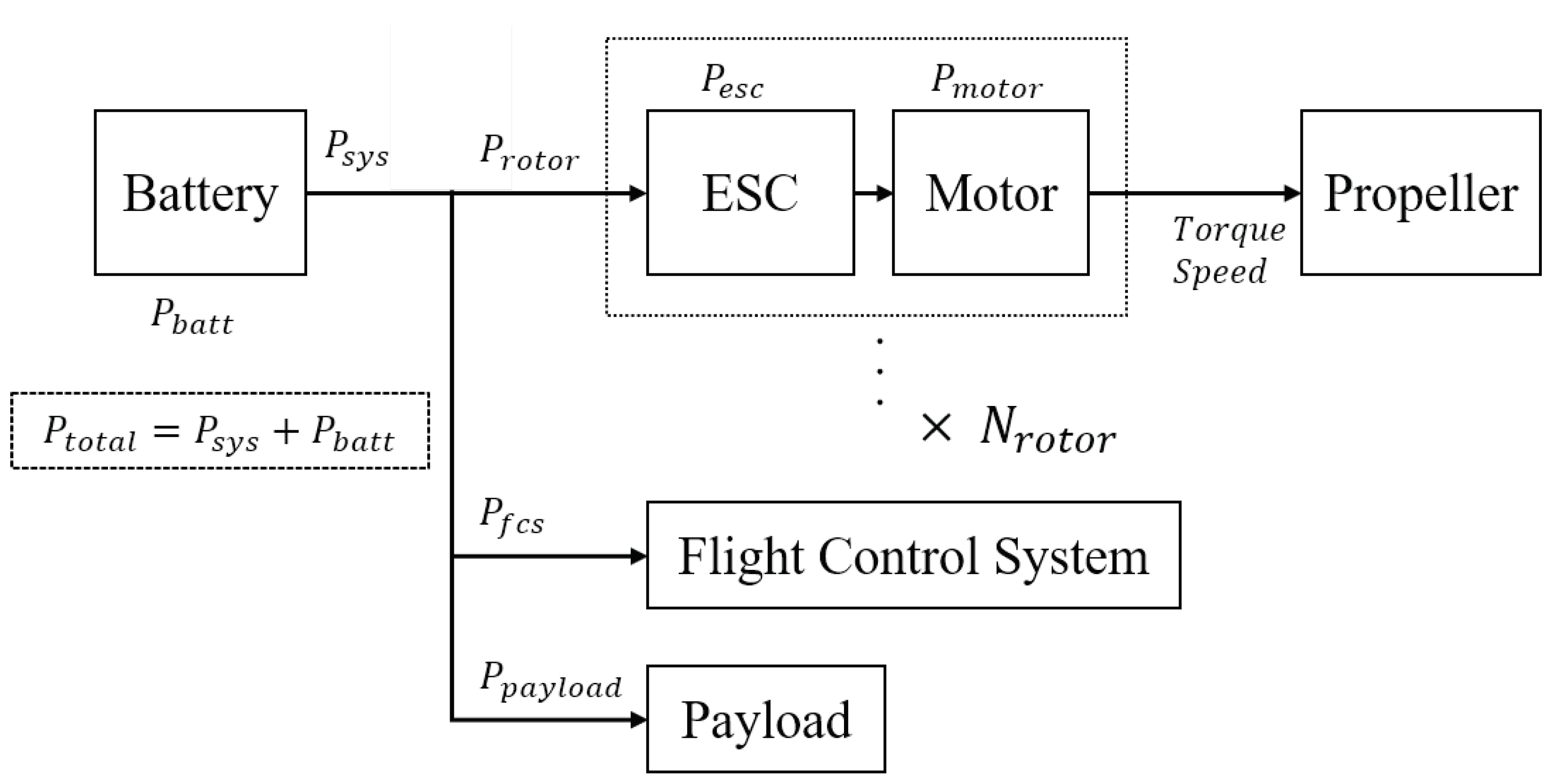
Figure 3.
Equivalent circuit of DC motor.
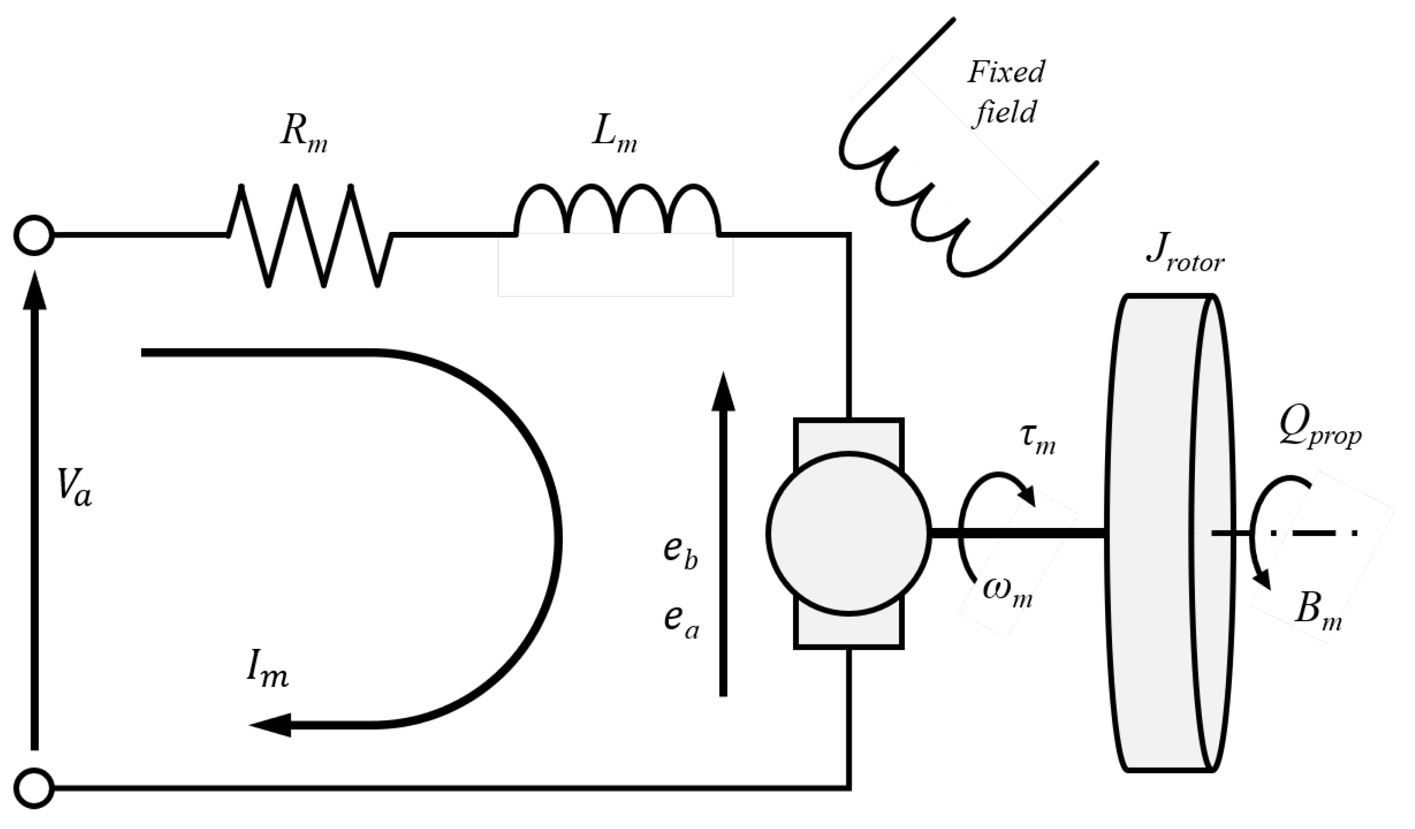
Figure 4.
Motor size constant vs viscous friction coefficient.
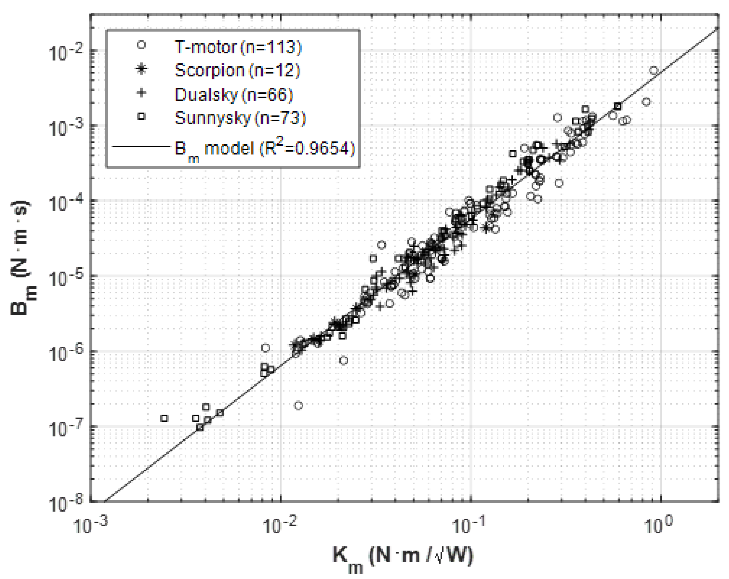
Figure 5.
Distortion of main field flux due to armature flux.

Figure 6.
Equivalent circuit of the electric speed controllers (ESC).

Figure 7.
Pulse width modulation (PWM) signal and phase voltage waveform for ideal trapezoidal commutation.
Figure 7.
Pulse width modulation (PWM) signal and phase voltage waveform for ideal trapezoidal commutation.
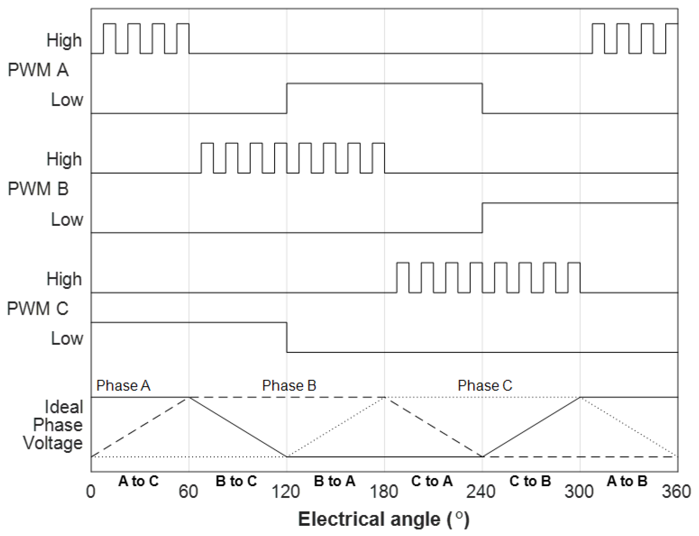
Figure 8.
Actual three phase voltage waveform measured by experiment.

Figure 9.
ESC continuous current vs. on-state resistance.

Figure 10.
Simple battery model.
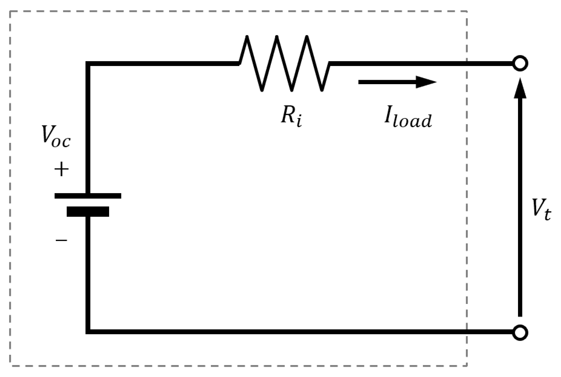
Figure 11.
Single cell LiPo battery battery samples.

Figure 12.
Average open-circuit voltage curve of the sample LiPo battery cells.
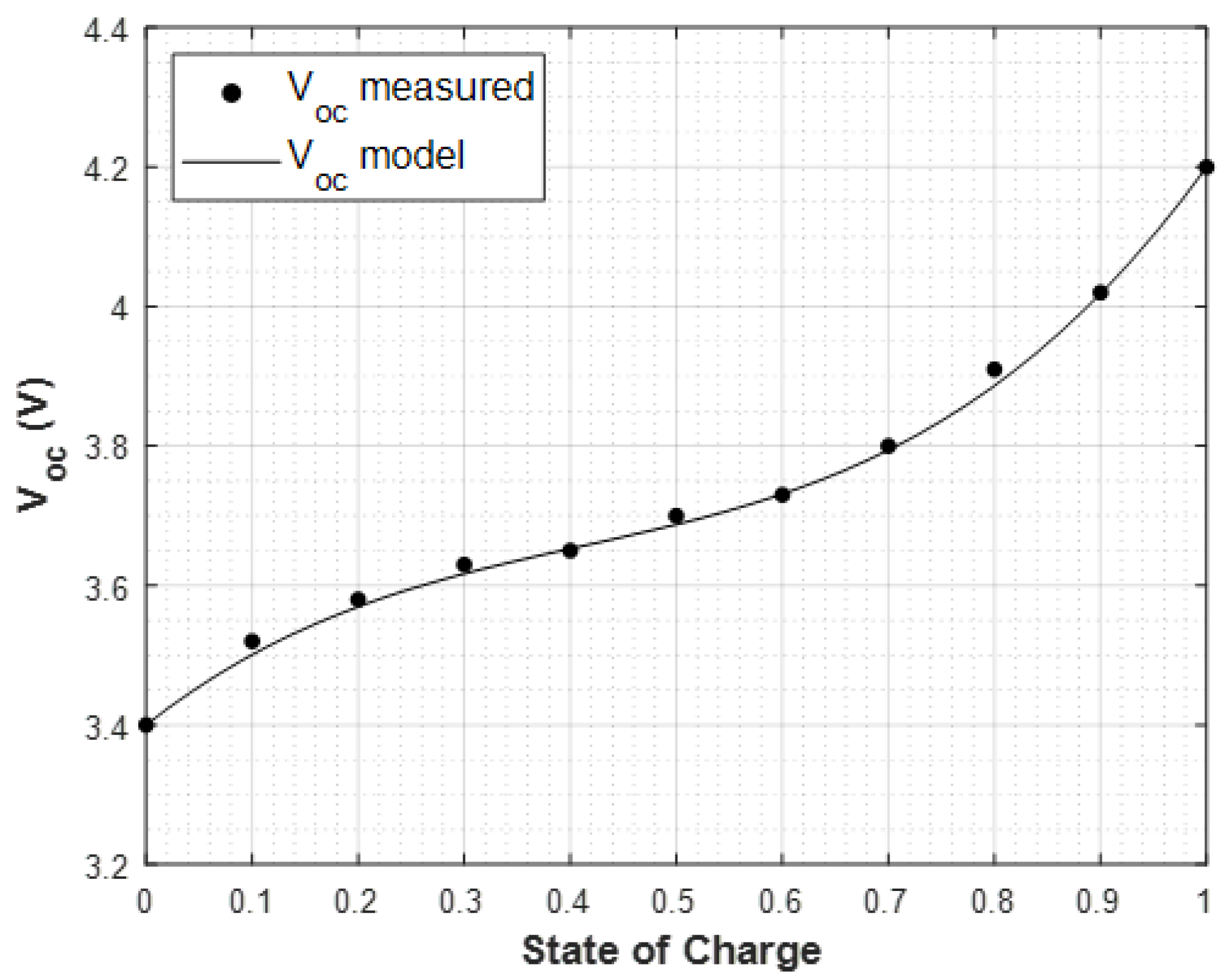
Figure 13.
Internal resistance of the Single cell LiPo battery samples according to the capacity.
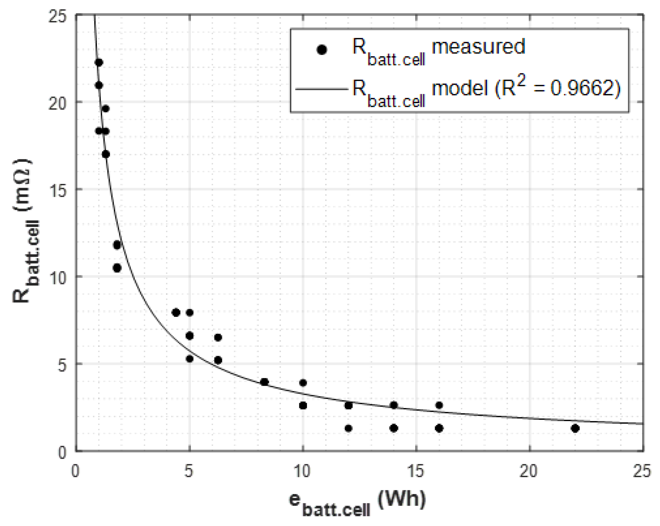
Figure 14.
Extended design structure matrix for the performance calculation process of the proposed electric propulsion system model.
Figure 14.
Extended design structure matrix for the performance calculation process of the proposed electric propulsion system model.

Figure 15.
diagram for the proposed performance calculation process of the electric propulsion system model.
Figure 15.
diagram for the proposed performance calculation process of the electric propulsion system model.
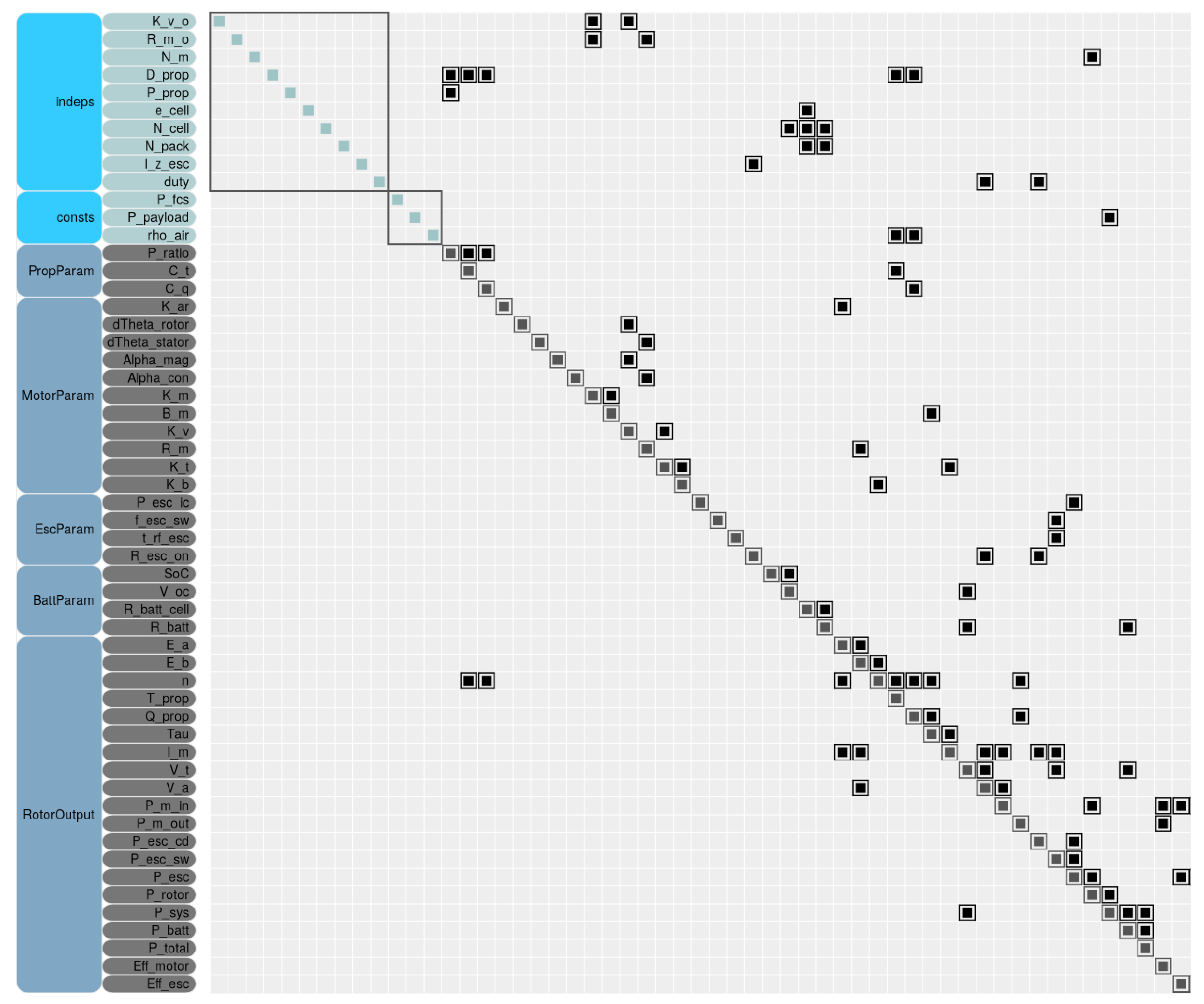
Figure 16.
Configuration of the thrust stand: (a) RCbenchmark Series 1780. (b) DAQ structure diagram.
Figure 16.
Configuration of the thrust stand: (a) RCbenchmark Series 1780. (b) DAQ structure diagram.

Figure 17.
Thermal imaging for measuring motor temperature change: (a) Motor stator temperature (≈), (b) Motor rotor temperature (≈).
Figure 17.
Thermal imaging for measuring motor temperature change: (a) Motor stator temperature (≈), (b) Motor rotor temperature (≈).
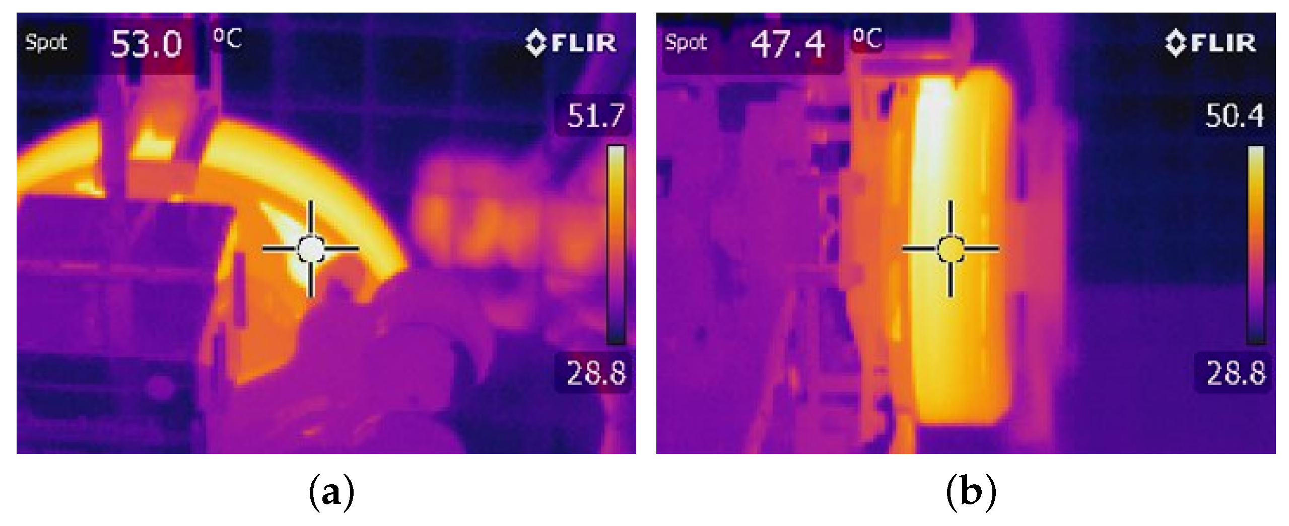
Figure 18.
Static thrust test results of sample set 1 (T-motor U15II with T-motor G40x13.1CF) compared with the datasheet: (a) Thrust, (b) torque, (c) rotational speed (d) terminal voltage (e) current consumption, and (f) power input.
Figure 18.
Static thrust test results of sample set 1 (T-motor U15II with T-motor G40x13.1CF) compared with the datasheet: (a) Thrust, (b) torque, (c) rotational speed (d) terminal voltage (e) current consumption, and (f) power input.
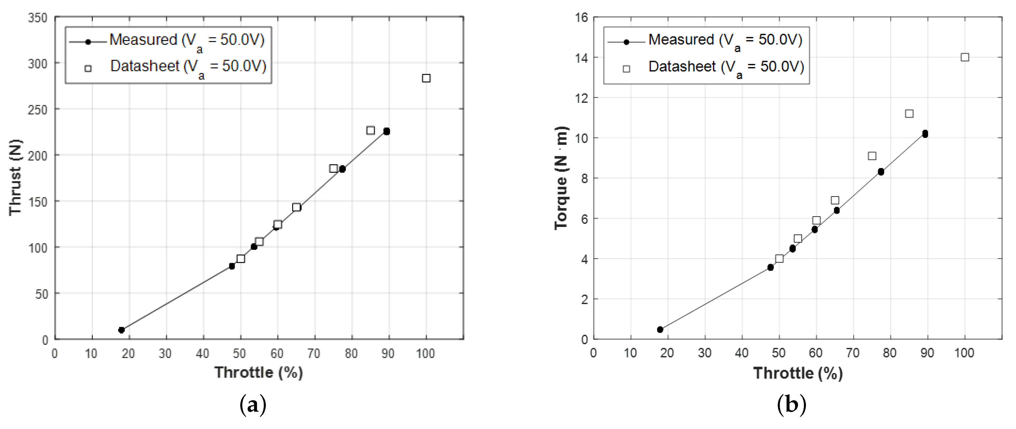

Figure 19.
Static thrust test results of sample set 2 (KDE13218XF-105 with KDE-CF-355-DP) compared with datasheet: (a) Thrust, (b) torque, (c) rotational speed, (d) terminal voltage, (e) current consumption, and (f) power input.
Figure 19.
Static thrust test results of sample set 2 (KDE13218XF-105 with KDE-CF-355-DP) compared with datasheet: (a) Thrust, (b) torque, (c) rotational speed, (d) terminal voltage, (e) current consumption, and (f) power input.
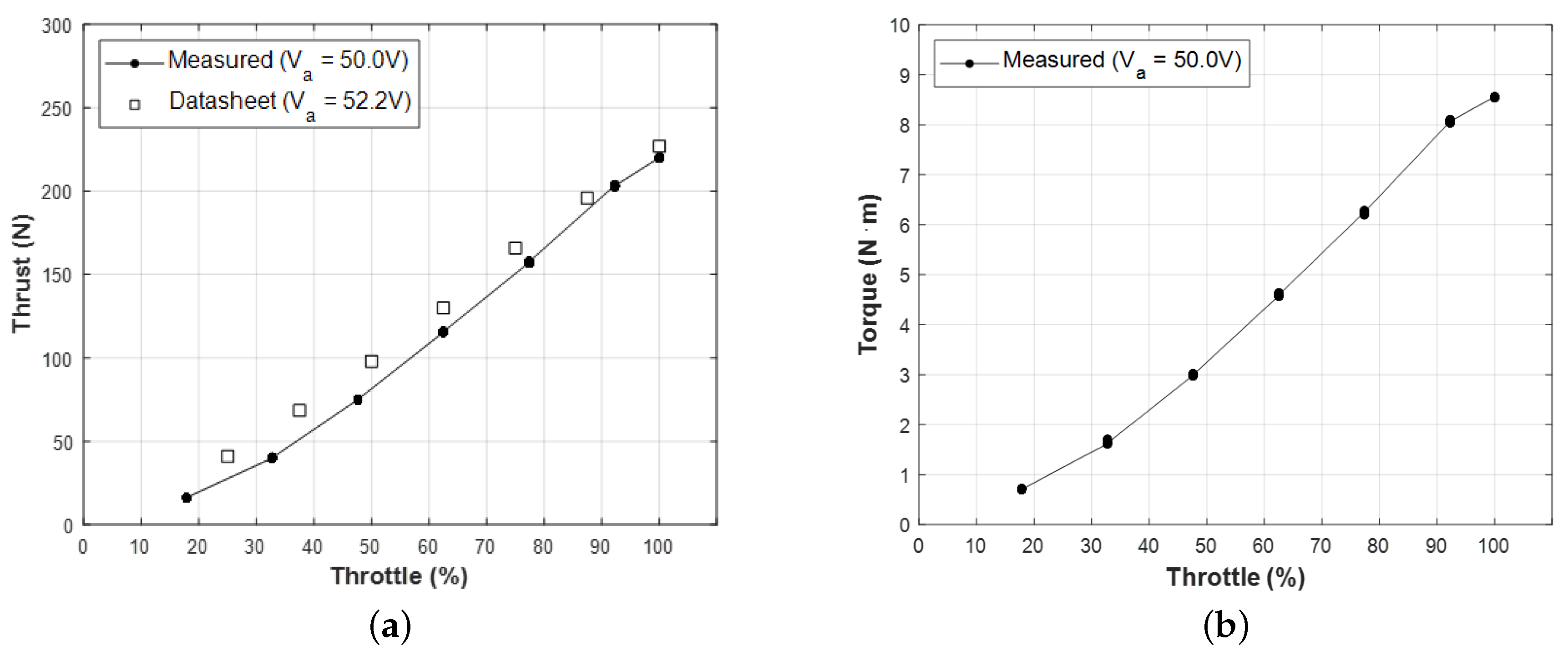
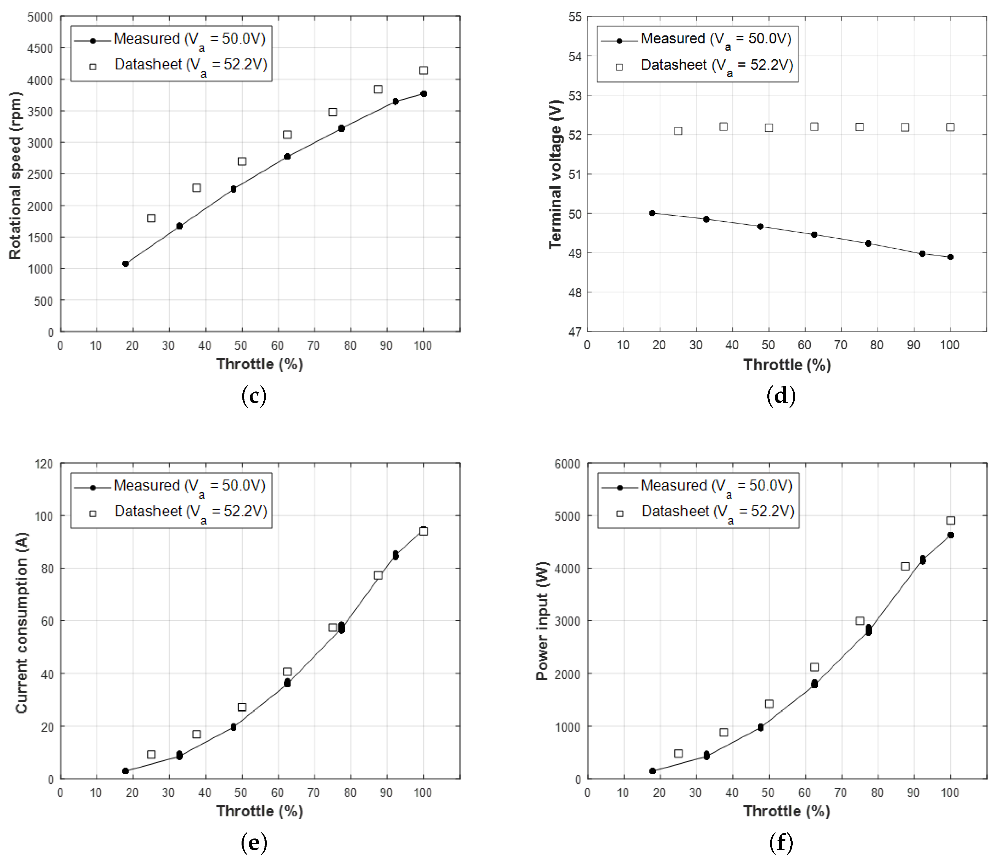
Figure 20.
Static thrust test results of sample set 3 (KDE10218XF-105 with KDE-CF-305-DP) compared with datasheet: (a) Thrust, (b) torque, (c) rotational speed, (d) terminal voltage, (e) current consumption, and (f) power input.
Figure 20.
Static thrust test results of sample set 3 (KDE10218XF-105 with KDE-CF-305-DP) compared with datasheet: (a) Thrust, (b) torque, (c) rotational speed, (d) terminal voltage, (e) current consumption, and (f) power input.


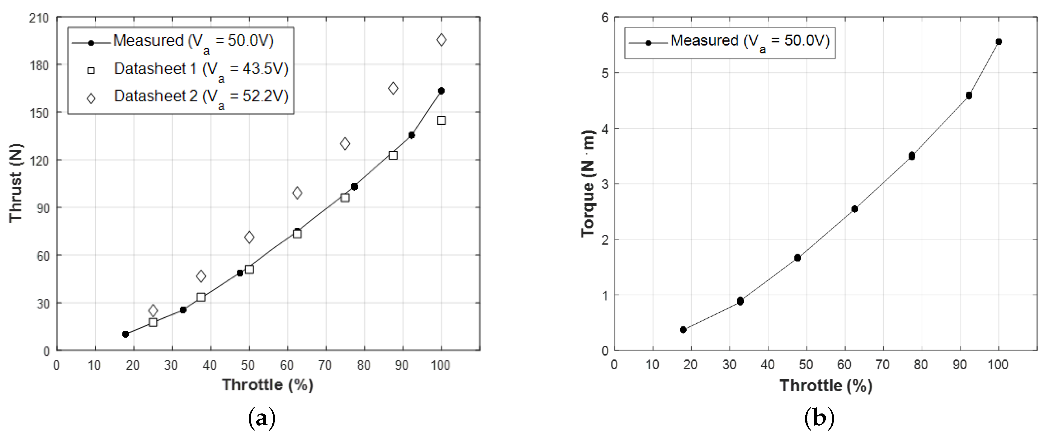
Figure 21.
Sample propeller thrust and torque model: (a) Thrust; (b) Torque.
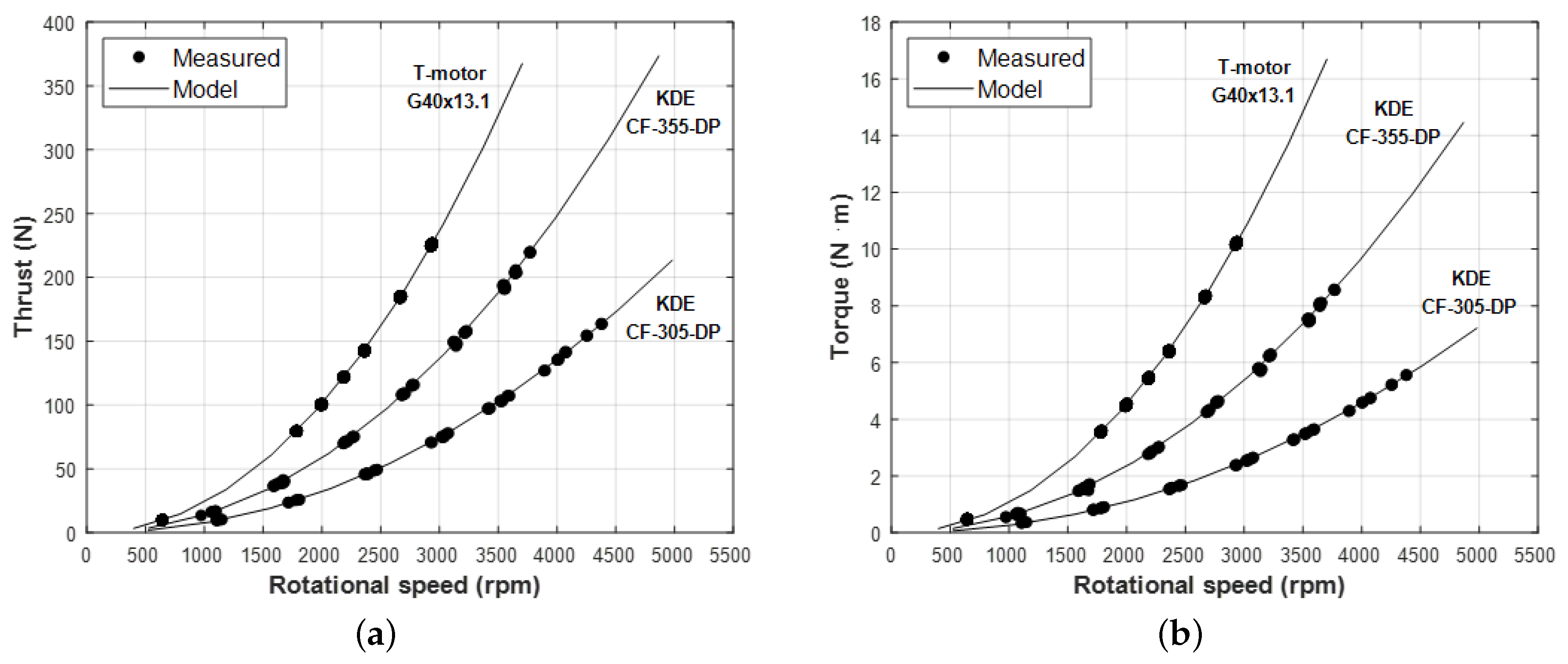
Figure 22.
Thermal profile for sample motors during the static thrust tests according to throttle inputs.
Figure 22.
Thermal profile for sample motors during the static thrust tests according to throttle inputs.
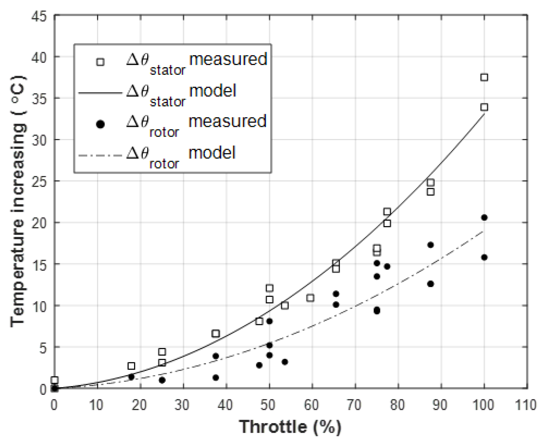
Figure 23.
Terminal voltage of the battery model and the power Supply according to the current load.
Figure 23.
Terminal voltage of the battery model and the power Supply according to the current load.
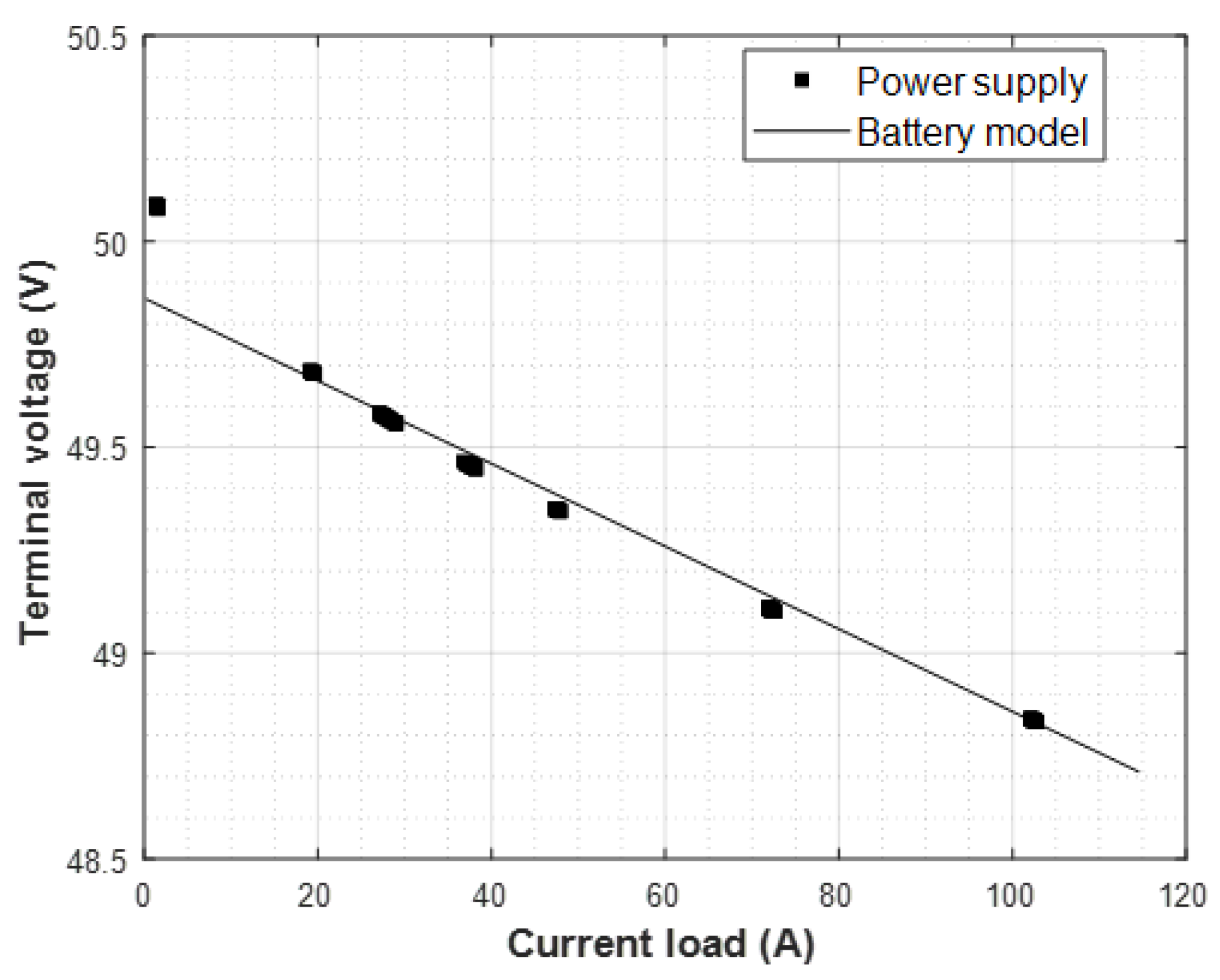
Figure 24.
Performance prediction results of sample set 1 (T-motor U15II with T-motor G40x13.1) compared with static thrust test results: (a) Thrust, (b) torque, (c) rotational speed, (d) terminal voltage, (e) current consumption, and (f) power input.
Figure 24.
Performance prediction results of sample set 1 (T-motor U15II with T-motor G40x13.1) compared with static thrust test results: (a) Thrust, (b) torque, (c) rotational speed, (d) terminal voltage, (e) current consumption, and (f) power input.
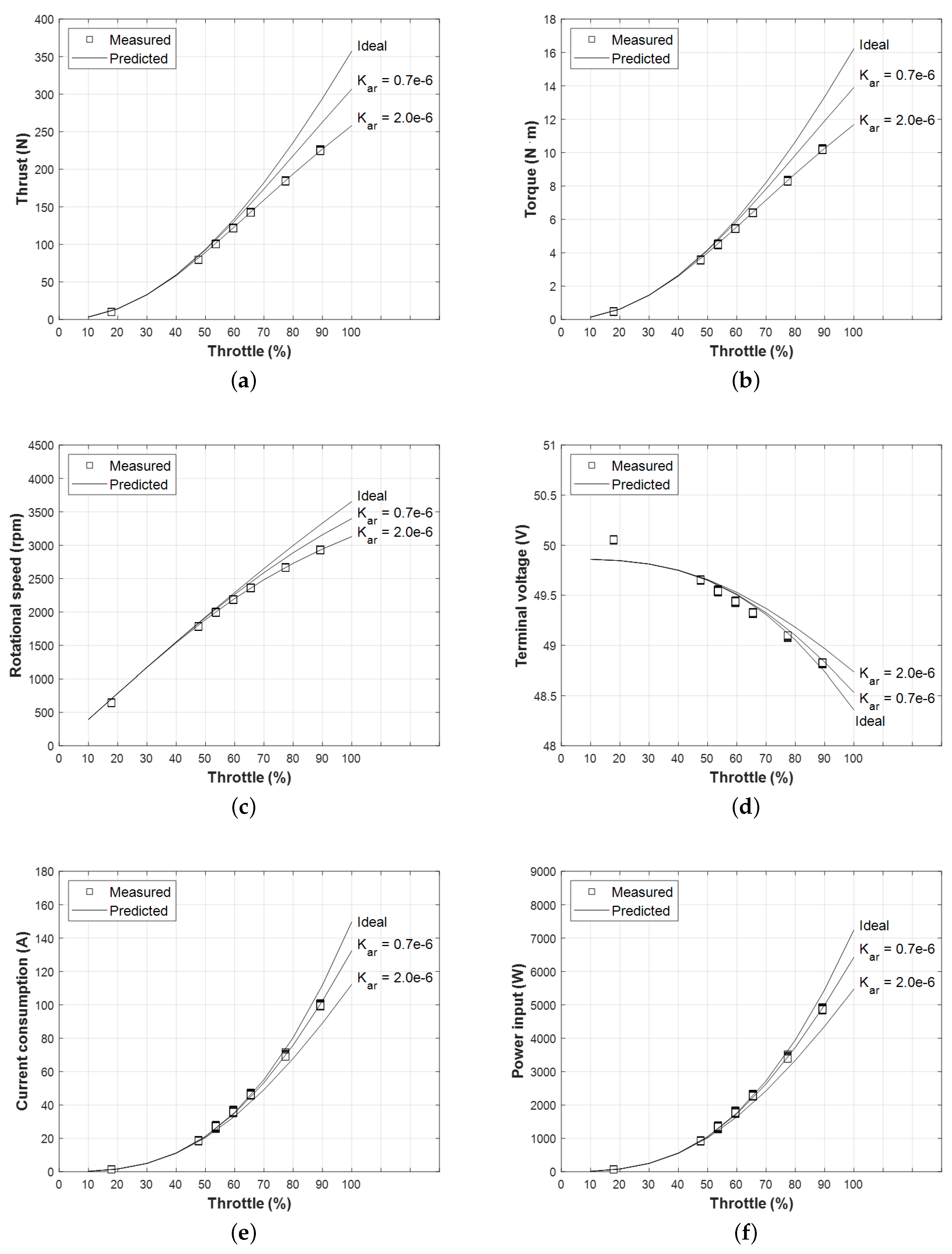
Figure 25.
Performance prediction results of sample set 2 (KDE13218XF-105 with KDE-CF-355-DP) compared with static thrust test results: (a) Thrust, (b) torque, (c) rotational speed, (d) terminal voltage, (e) current consumption, and (f) power input.
Figure 25.
Performance prediction results of sample set 2 (KDE13218XF-105 with KDE-CF-355-DP) compared with static thrust test results: (a) Thrust, (b) torque, (c) rotational speed, (d) terminal voltage, (e) current consumption, and (f) power input.
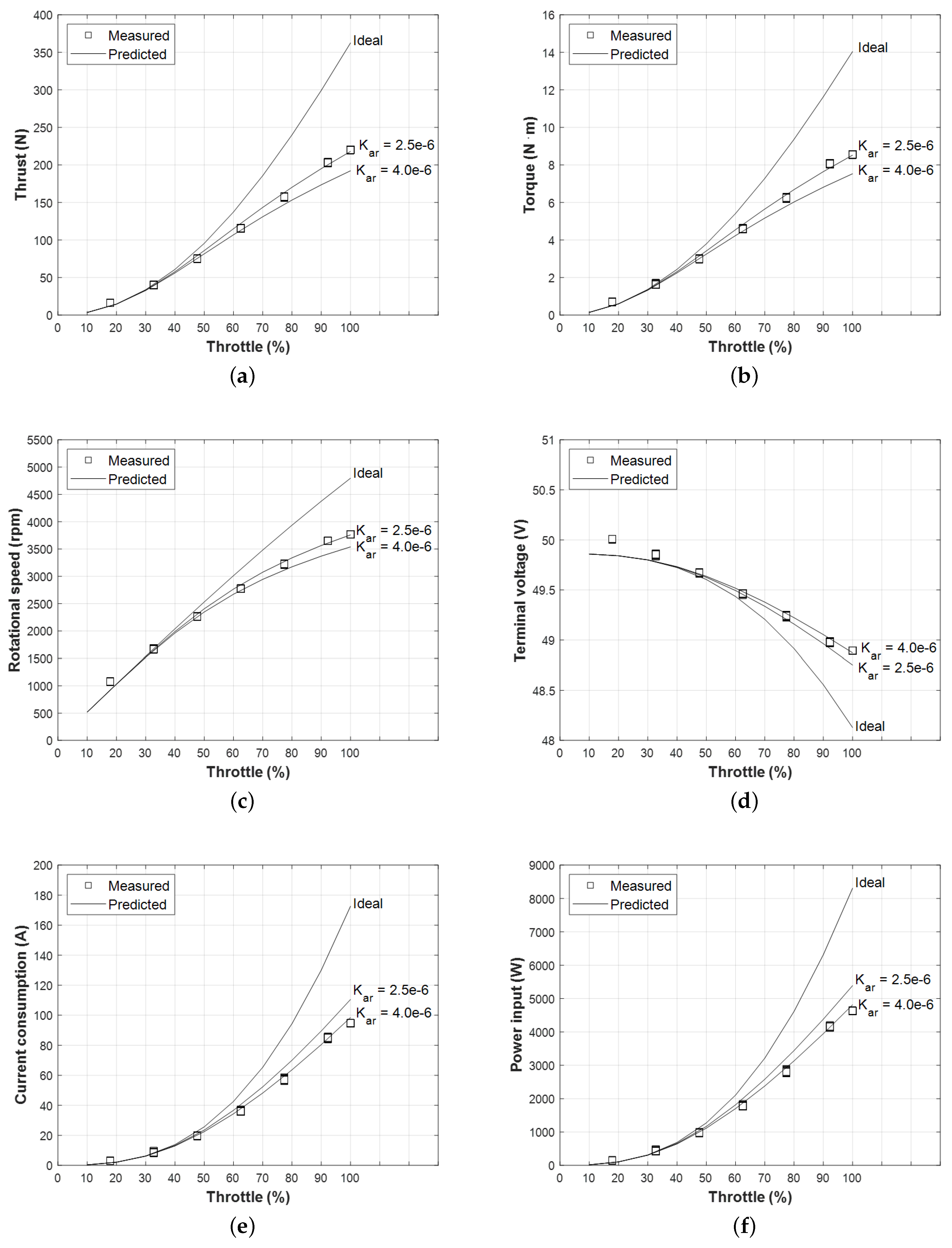
Figure 26.
Performance prediction results of sample set 3 (KDE10218XF-105 with KDE-CF-305-DP) compared with static thrust test results: (a) Thrust, (b) torque, (c) rotational speed, (d) terminal voltage, (e) current consumption, and (f) power input.
Figure 26.
Performance prediction results of sample set 3 (KDE10218XF-105 with KDE-CF-305-DP) compared with static thrust test results: (a) Thrust, (b) torque, (c) rotational speed, (d) terminal voltage, (e) current consumption, and (f) power input.


Table 1.
Magnet temperature coefficient and temperature limit for various magnet types.
| Magnet Type | Ceramic | SmCo | AlNiCo | NdFeB |
|---|---|---|---|---|
| [/C] | −0.0020 | −0.0004 | −0.0002 | −0.0012 |
| [C] | 300 | 300 | 540 | 150 |
Table 2.
Conductor temperature coefficient for various materials.
| Conductor Material | Silver | Gold | Copper | Aluminum |
|---|---|---|---|---|
| [/C] | 0.0038 | 0.0037 | 0.0040 | 0.0043 |
Table 3.
Commercial multicopter dedicated ESCs and metal oxide semiconductor field-effect transistors (MOSFETs) specification samples.
Table 3.
Commercial multicopter dedicated ESCs and metal oxide semiconductor field-effect transistors (MOSFETs) specification samples.
| Item | 1 | 2 | 3 | 4 | 5 | 6 |
|---|---|---|---|---|---|---|
| Manufacturer | T-motor | T-motor | T-motor | T-motor | CobraMotor | STM |
| Product | Flame60A HV | Flame100A LV | Flame100A HV | Flame200A HV | MR60 | ESC001V1 |
| Max. Current | 60 A | 100 A | 100 A | 200 A | 60 A | 20 A |
| Peak Current | 80 A | 120 A | 120A | 240 A | 75 A | 30 A |
| Max. Voltage | 52.2 V | 34.8 V | 60.9V | 60.9 V | 26.1 V | 26.1 V |
| Max. Power | 3132 W | 3480 W | 6090 W | 12180 W | 1566 W | 522 W |
| MOSFET | TPR4R008NH | FDMS8333L | IPB015N08N5 | TPH4R50ANH | TPCA8057-H | STL160N4F7 |
| No. of MOSFETs | 18 | 30 | 6 | 42 | 18 | 6 |
| 3.3 m | 2.4 m | 1.1 m | 3.7 m | 2.6 m | 2.1 m | |
| 2.2 m | 0.96 m | 2.2 m | 1.057 m | 1.733 m | 4.2 m | |
| 5.7 nSec | 4.7 nSec | 32.0 nSec | 9.6 nSec | 4.3 nSec | 6.6 nSec | |
| 11.0 nSec | 4.2 nSec | 28.0 nSec | 13.0 nSec | 6.3 nSec | 5.7 nSec | |
| Item | 7 | 8 | 9 | 10 | 11 | 12 |
| Manufacturer | Hobbywing | Hobbywing | Hobbywing | Hobbywing | Hobbywing | Hobbywing |
| Product | XRotor10A | XRotor15A | XRotor20A | XRotor25A | XRotor40A Pro | XRotor50A Pro |
| Max. Current | 10 A | 15 A | 20 A | 25 A | 40 A | 50 A |
| Peak Current | 15 A | 20 A | 30 A | 40 A | 60 A | 70 A |
| Max. Voltage | 13.05 A | 17.4V | 17.4 V | 26.1 V | 26.1 V | 26.1 V |
| Max. Power | 130.5 W | 261 W | 348 W | 652.5 W | 1044 W | 1305 W |
| MOSFET | IRFH830PbF | IRFH8318PbF | TPCA8087 | IRFH7440PbF | FDMS8333L | SM4023NSKP |
| No. of MOSFETs | 6 | 6 | 6 | 6 | 12 | 12 |
| 3.0 m | 2.5 m | 1.5 m | 1.8 m | 2.4 m | 1.85 m | |
| 6.0 m | 5.0 m | 3.0 m | 3.6 m | 2.4 m | 1.85 m | |
| 25.0 nSec | 33.0 nSec | 5.7 nSec | 45.0 nSec | 4.7 nSec | 10.0 nSec | |
| 9.2 nSec | 12.0 nSec | 11.0 nSec | 42.0 nSec | 4.2 nSec | 34.0 nSec |
: 4.35 V × Max. cell number of support LiPB, : Max.Voltage × Max.Current, : Typical value provided in datasheet, : /(No. of MOSFET/3).
Table 4.
Sample sets for model validation.
| Specifications | Set 1 | Set 2 | Set 3 | |
|---|---|---|---|---|
| Motor | Product | T-motor U15II | KDE13218XF-105 | KDE10218XF-105 |
| (rpm/V) | 80 | 105 | 105 | |
| (m) | 17 | 13 | 23 | |
| (A @ 10 V) | 3.8 | 3.1 | 1.0 | |
| Propeller | Product | T-motor G404 × 13.1CF | KDE-CF-355-DP 35.5 × 12.1 | KDE-CF-305-DP 30.5 × 9.7 |
| Dia. (inches) | 40 | 35.5 | 30.5 | |
| Pitch (inches) | 13.1 | 12.1 | 9.7 | |
| ESC | Product | FLAME 180A HV | KDE-UAS125UVC-HE | |
| (A) | 180 | 125 | ||
| Power | Experiment | Power supply (Capacity: 12,000 W) | ||
| Model | LiPo Battery (12S1P 18,000 mAh) | |||
Table 5.
Static thrust and torque coefficient model for sample propellers (Equation (7)).
Table 5.
Static thrust and torque coefficient model for sample propellers (Equation (7)).
| Sample | Coefficient | k [m s] | a [ ] | b [ ] | c [ ] |
|---|---|---|---|---|---|
| T-motor G40x13.1 | 0.075880 | 0.09323 | 0.1316 | 0.3516 | |
| 0.006009 | 0.01175 | 0.4024 | 0.9575 | ||
| KDE-CF-355-DP | 0.076060 | 0.08517 | 0.1927 | 0.3854 | |
| 0.007588 | 0.04714 | 0.4976 | 0.9844 | ||
| KDE-CF-305-DP | 0.080430 | 0.07712 | 0.1793 | 0.3577 | |
| 0.007955 | 0.07292 | 0.4924 | 0.9867 |
Publisher’s Note: MDPI stays neutral with regard to jurisdictional claims in published maps and institutional affiliations. |
© 2020 by the authors. Licensee MDPI, Basel, Switzerland. This article is an open access article distributed under the terms and conditions of the Creative Commons Attribution (CC BY) license (http://creativecommons.org/licenses/by/4.0/).
Share and Cite
MDPI and ACS Style
Jeong, J.; Shi, H.; Lee, K.; Kang, B. Improvement of Electric Propulsion System Model for Performance Analysis of Large-Size Multicopter UAVs. Appl. Sci. 2020, 10, 8080. https://doi.org/10.3390/app10228080
AMA Style
Jeong J, Shi H, Lee K, Kang B. Improvement of Electric Propulsion System Model for Performance Analysis of Large-Size Multicopter UAVs. Applied Sciences. 2020; 10(22):8080. https://doi.org/10.3390/app10228080
Chicago/Turabian StyleJeong, Jinseok, Hayoung Shi, Kichang Lee, and Beomsoo Kang. 2020. "Improvement of Electric Propulsion System Model for Performance Analysis of Large-Size Multicopter UAVs" Applied Sciences 10, no. 22: 8080. https://doi.org/10.3390/app10228080
Note that from the first issue of 2016, this journal uses article numbers instead of page numbers. See further details here.