Stress-Based Weibull Method to Select a Ball Bearing and Determine Its Actual Reliability

Featured Application

Based on the catalogue L₁₀ life, the paper let us to select the ball bearing that corresponds to the analyzed application, both formulation and steps are given. Moreover, when the actual application conditions are different of those at which the ball bearing was designed, the proposed method let practitioners to determine the real L-life (or reliability) that corresponds to the actual conditions, a step by step application and formulation is presented. Additionally, this methodology can be applied to any field or application where the input variables are either contact stress or principal stress values.

Abstract

Since the designed bearing’s reliability of 90% was determined in a lab environment, it does not represent the actual used environment. In this paper, a new methodology to determine the actual reliability that corresponds to the use conditions is offered. This new method is based on the standard method used to select the ball bearing. The proposed method is based on the two parameters of Weibull distribution, where the shape (β) and scale (η) parameters are both determined from the Hertz contact stresses values, which are generated under the surface of the motionless outer race, and by the forces transmitted between the ball and the outer race. Therefore, the derived reliability is different from the 90% index offered by manufacturers.

1. Introduction

Ball bearings are important machine components that are used in vehicles, machines, airplanes, appliances, and precision equipment [1,2]. Defects of ball bearings are the main cause of failure of a rotating machine [3,4]. A ball bearing failure caused a mechanical machine to stop working, resulting in economic losses. Therefore, fatigue life prediction for bearing has an important significance and practical value [5]. Currently, bearing manufactures offer their products with a reliability based on the L₁₀ life percentile, that is obtained through tests performed on static loads and at a certain rotation speed [6]. Therefore, machine designers and people who use machines need to know the actual reliability that corresponds to their own application. In various articles, Erwing Zarestsky explained how the L₁₀ life equation has been analyzed in different models such as the Waloddi Weibull fatigue life model, Lundberg-Palmgren model, Ionnides-Harris model, and Zaretsky model [7,8,9]. In 1962, The Lundberg-Palmgren life equation has been incorporated into the International Organization for Standardization (ISO). Over the years, the formula has been questioned for various reasons, one of which is that it was obtained by testing bearings of the same model and under laboratory conditions. The aim of this article is not to criticize the formula, but rather, to make use of it in a new methodology to obtain the reliability in a current ball bearing application. The actual reliability must be different from the reliability offered in the L₁₀ life equation.

Consequently, in this article, a new methodology to determine the reliability of a ball bearing in its actual application is given. The proposed method is based on the generated Hertz contact stresses values, which are present on the fixed outer ring race.

Moreover, this proposed method is based on the traditional method to select a ball bearing, and in Hertz theory, both methods let us determine the magnitude of the generated contact stresses. Then, based on these Hertz stresses values, the parameters shape beta (β) and scale eta (η) parameters of the Weibull distribution are determined. Finally, by using them, the corresponding actual ball bearing reliability is determined. Consequently, since the actual reliability index is based on the generated stresses, then the proposed methodology can also be used to determine the reliability of a single-row deep groove ball bearings application.

The present work is organized as follows. Section 2 explains the Hertz theory. Section 2.1 describes the steps to determine the contact stresses and the L₁₀ life of a ball bearing, while Section 2.2 describes the steps to determine the contact area of a ball bearing. In Section 2.3, the steps to determine the principal stresses are given. Section 2.4 shows how to determine the Weibull shape β and scale η parameters, and Section 2.5 shows the steps to determine the actual reliability of the selected ball bearing. In Section 3, an application of the new methodology is presented. Finally, in Section 4, the conclusions are given.

2. Hertz Contact Generalities

In 1879, Heinrich Hertz found that the way to determine the stresses on the surface of rolling bodies was only through an approximation, which was done using a set of empirical assumptions. In 1881, Hertz proposed the contact stress theory or Hertz theory. This theory is a mathematical analysis of the relationship between the shape of the geometry, the size of the contact area, and the distribution of the stresses in two bodies with curved surfaces. Later, some researchers added to the existing theory the fact that the maximum stresses that cause the ball bearings to break are generated below the contact surface [7,10,11,12,13]. Contact stresses occur when two bodies transmit loads across their surfaces, generating a point or a line contact [14]. There are three ways in which contact forces can occur: The first is when a sphere or a roller is pressed on a flat surface, the second occurs when two spheres or two rollers are pressed against each other, and the third is when a roller or a sphere is pressed against a concave curved surface. When applying a force on two bodies, the surface that is in contact flattens out and takes an elliptical, circular, or rectangular shape, this depends on the shape of the bodies that are in contact. In the case analyzed in this article, the contact between a ball and the outer race, generates an elliptical contact surface. Therefore, it meets the conditions to apply the Hertz theory. Among these conditions, we have that (a) the materials of both bodies must be homogeneous and isotropic, (b) the contact areas are relatively small compared to the curvature radius, (c) the contact surfaces have an elastic behavior, and (d) loads are normal to contact surfaces [13,15,16].

On the other hand, from the Weibull analysis performed to determine the life of the bearing, the generated contact stresses are used to determine the corresponding Weibull parameters. Then, the relevant stresses are the main stresses σ_x, σ_y, σ_z and the maximum shear stress τ_max that are generated below the bearing surface [13]. Note that at the point where τ_max occurs, the cracking occurs in the outer race and that generates the failure. Therefore, the analysis is performed on the outer race of the ball bearing. The analysis is as follows.

2.1. Steps to Determine the Contact Stresses and the L₁₀ Life of a Ball Bearing Subsection

Step 0. Determine the loads that are acting on the ball bearings.

Step 1. From the static shaft analysis, determine the design P_d load at which the ball bearing will be subjected. By using the radial (F_r) and axial (F_a) forces determined in the static shaft analysis, with the X radial and Y axial ball bearing coefficients given in the selected ball bearings’ catalogues, determine the equivalent radial load p-value from Equation (1) as:

$$P=X{F}_r+Y{F}_a$$

(1)

then, by using the P radial force with the rotation factor V, determine the design load value as:

$$P_d=VP$$

(2)

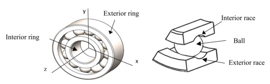
Note that from Equation (2) if the interior race is rotating, then V = 1 and, in contrast, if the exterior ring is rotating, then V = 1.2 (see Figure 1).

Figure 1. Interior and exterior rings and interior and exterior races of a ball bearing.

Note 1: The P_d-value in Equation (2) is determined in the static phase analysis and, is done based on the applied loads that correspond to the point where the ball bearing is going to be mounted.

Step 2. Select the ball bearing, which can be selected from a catalogue. To do this, the type of ball bearing that corresponds to the application is first determined. In this paper, a deep groove ball bearing is used. To select it from the catalogues, the catalogues’ diameter must be the shaft’s diameter value where the ball bearing is going to be mounted. In addition, the designed load P_d addressed in step 1 must be lower than the catalogues’ dynamic load (C). If C is lower than P_d, another type of ball bearing must be selected. Similarly, the rotation speed at which the ball bearing is going to be mounted must be lower than the one given in the catalogue. Additionally, the P_d-value has to be lower than the basic static load (C_o) of the catalogue.

Step 3. Determine the designed L₁₀ life of the ball bearing. By using C from step 2 and P_d from step 1, the ball bearing L₁₀ life is given as [2,17]:

$$L_{10}={10}^6{\left(\frac{C}{Pd}\right)}^3$$

(3)

where L₁₀ represents the expected number of cycles at which 10% of the ball bearings will fail.

2.2. Steps to Determine the Contact Area of the Ball Bearing

Step 4. Determine the total curvature R of the contact area. In this case, the curvature analysis is performed between the outer race and the ball bearing. From this analysis, the total curvature R is determined based on the ball bearing dimensions, the inner race radius, and on the radius of the ball bearing [12,18]. Since in a ball bearing the curvature is generated in the x and y directions, then the total curvature is given as:

$$\frac{1}{R}=\frac{1}{R_x}+\frac{1}{R_y}$$

(4)

where:

$$\frac{1}{R_x}=\frac{1}{r_{ax}}+\frac{1}{r_{bx}}$$

(5)

$$\frac{1}{R_y}=\frac{1}{r_{ay}}+\frac{1}{r_{by}}$$

(6)

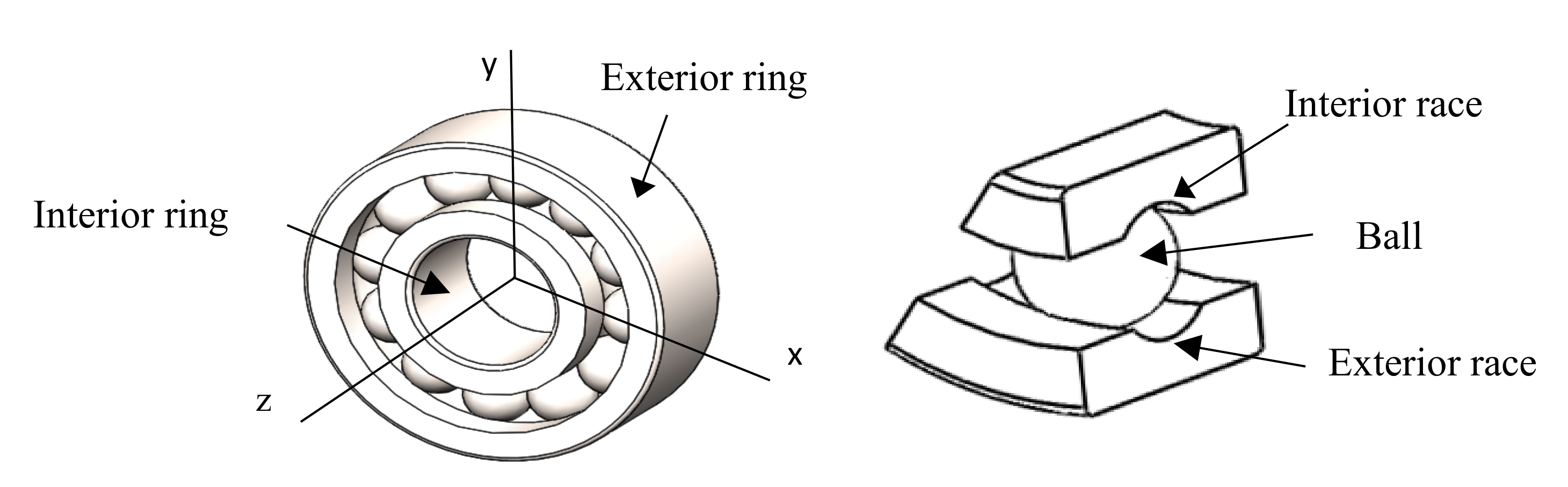
In addition, since r_ax and r_ay are the radius of the ball in the x and y direction, respectively, then r_ax = r_ay. Moreover, r_bx is the curvature radius from the center of the ball bearing to the race of the exterior ring, and r_by is the curvature radius of the race of the exterior ring (see Figure 2). As seen in Figure 1, a ball bearing has two races, one in the exterior ring and one in the inner ring. Note that the analysis is performed over the race of the outer ring due to fact that the distribution of the load between the race of the exterior ring and the ball is higher than between the race of the inner ring and the ball [19].

Figure 2. Ratio of the ball and the race of the exterior ring.

Nevertheless, since most of the catalogues do not contain the radius of the race of the exterior ring, then it is determined as in Equation (7), where $R_r$ is the race conformity of the race of the exterior ring with a standardized value of 0.52 [17,20], and d_B is the ball diameter. Therefore, the race of the exterior ring r_by radius is given as:

$$R_r=\frac{r_{by}}{d_B}$$

(7)

Step 5. Determine the curvature’s index α_r as:

$${\alpha }_r=\frac{R_y}{R_x}$$

(8)

Step 6. Determine the elliptical parameter k_e as:

$$k_e={\left({\alpha }_r\right)}^{\raisebox{1ex}{$2$}\!\left/ \!\raisebox{-1ex}{$\pi $}\right.}$$

(9)

Step 7. From Table 1, select the elliptical equations to be used to determine the a and b axes of the contact ellipse, as mentioned from step 7.1 to step 9.

Table 1. Simplified equations of the ellipticals integrals.

	Range of the Curvature’s Radius
Property	(1 ≤ αr ≤ 100)	(0.01 ≤ αr ≤ 1)
Geometry
Ellipticity ratio	$k_e={\alpha }_r{}^{\raisebox{1ex}{$2$}\!\left/ \!\raisebox{-1ex}{$\pi $}\right.}$	$k_e={\alpha }_r{}^{\raisebox{1ex}{$2$}\!\left/ \!\raisebox{-1ex}{$\pi $}\right.}$
Elliptical integer of first order $\mathcal{F}$	$\mathcal{F}=\frac{\pi }{2}+\left(\frac{\pi }{2}-1\right)\ln {\alpha }_r$	$\mathcal{F}=\frac{\pi }{2}-\left(\frac{\pi }{2}-1\right)\ln {\alpha }_r$
Elliptical integer of second order $\mathcal{E}$	$\mathcal{E}=1+\frac{\pi -2}{2{\alpha }_r}$	$\mathcal{E}=1+\left(\frac{\pi }{2}-1\right){\alpha }_r$

Step 7.1. Determine the value of the simplified ellipticals integrals $\mathcal{F}$ y $\mathcal{E}$, given in Table 1, which are determined by using the curvature’s index α_r and the elliptical parameter k_e in the corresponding elliptical functions.

The elliptical integral functions of first order $\left(\mathcal{F}\right)$ and second order ($\mathcal{E}$), the geometry of the generated ellipse, and the ellipticity ratio ($k_e)$ all them depend on the curvature index α_r, in such a way that if 1 ≤ α_r ≤ 100, the equations from the left column of Table 1 [12] must be selected. In contrast if 0.01 ≤ α_r ≤ 1, the equations from the right column of Table 1 must be selected. From Table 1, also note that based on the α_r value and from the x and y axes of the generated contact ellipse, the a and b values are determined.

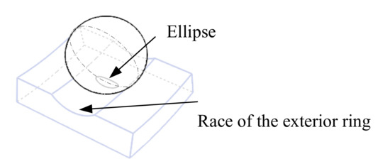
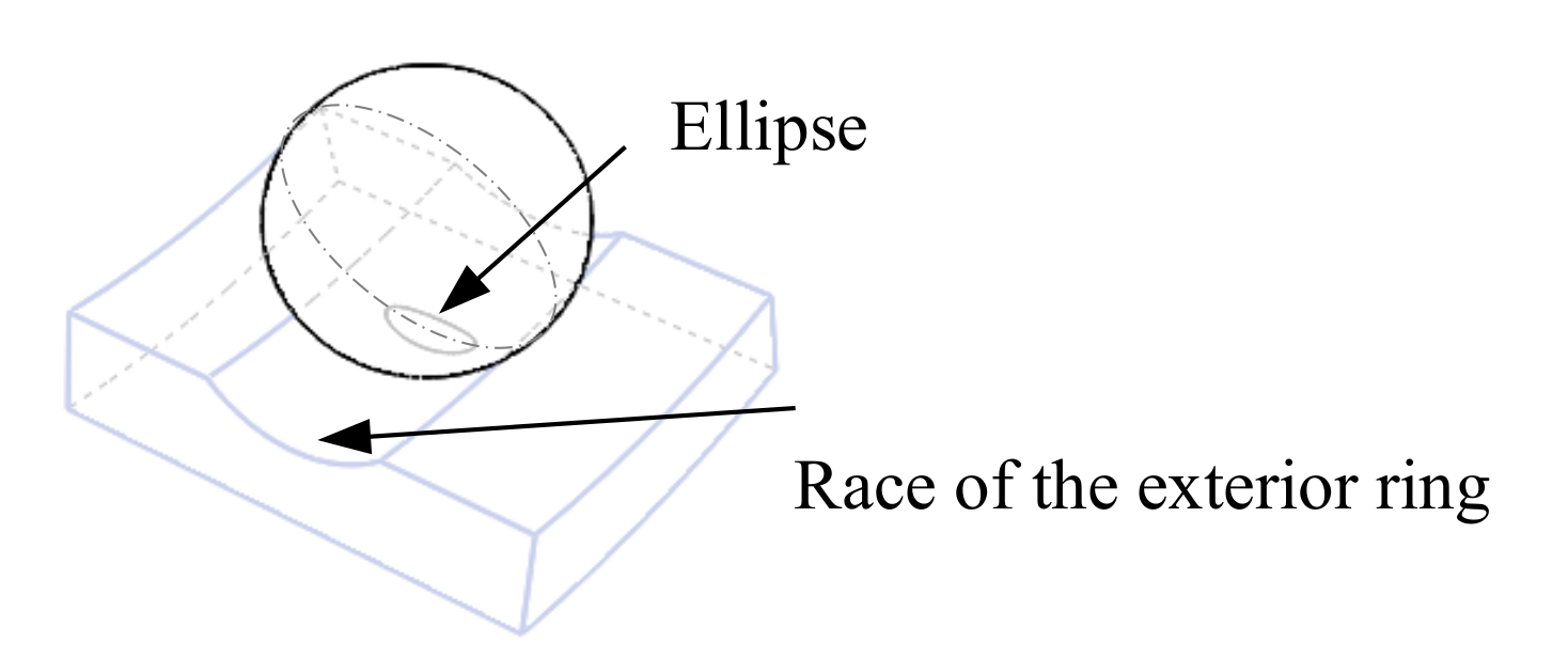
Here noticed that the contact ellipse area is generated when a force pressures the ball against the race of the exterior ring as shown in Figure 3.

Figure 3. Ellipse generated between the ball and the race of the exterior ring.

Step 8. Determine the effective elasticity module (E’). Based on the Poisson coefficient (v) and on the elasticity module (E) of the used materials, the effective elasticity module is given as:

$$E^{\prime }=\frac{2}{\frac{\left(1-v_a{}^2\right)}{E_a}+\frac{\left(1-v_b{}^2\right)}{E_b}}$$

(10)

In Equation (10), v_a is the Poisson coefficient of the ball, and v_b is the Poisson coefficient of the outer ring. Similarly, E_a is the elasticity module of the ball, and E_b is the elasticity module of the exterior ring.

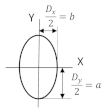
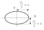
Step 9. Determine the a and b dimensions of the semiaxes of the ellipse. An ellipse is formed in the contact point between the ball and the race of the exterior ring (see Table 1). The a and b values are determined as one half of the dimensions of the (D_y) and (D_x) diameters of the ellipse given as:

$$D_y=2{\left(\frac{6k_e{}^2\mathcal{E}{P}_{d}R}{\pi E^{\prime }}\right)}^{\raisebox{1ex}{$1$}\!\left/ \!\raisebox{-1ex}{$3$}\right.}$$

(11)

$$D_x=2{\left(\frac{6\mathcal{E}{P}_{d}R}{\pi k_e{E}^{\prime }}\right)}^{\raisebox{1ex}{$1$}\!\left/ \!\raisebox{-1ex}{$3$}\right.}$$

(12)

Note 2. Note in the ellipse that “a” always represents the higher semi axis. For example, if D_y > D_x, then a = D_y/2 and b = D_x/2, in contrast if D_x > D_y, then a = D_x/2 and b = D_y/2.

Now based on the above dimensions, the values of the principal contact stresses have to be calculated. This is due to the fact that these values are used in the proposed method to determine the Weibull parameters, which are used to compute the actual ball bearing reliability.

2.3. Steps to Determine the Contact Principal Stresses Values

Step 10. Determine the maximum stress P_max value, which occurs in the contact point between the ball and the race of the exterior ring and is given as:

$$P_{max}=\frac{6P_d}{\pi D_x{D}_y}$$

(13)

Step 11. Determine the contact principal stresses σ_x, σ_y, σ_z, and τ_max values, which are given as:

$${\sigma }_x=\left[M\left({\mathsf{\Omega }}_x+v{{\mathsf{\Omega }}^{\prime }}_x\right)\right]\frac{b}{\Delta }$$

(14)

$${\sigma }_y=\left[M\left({\mathsf{\Omega }}_y+v{{\mathsf{\Omega }}^{\prime }}_y\right)\right]\frac{b}{\Delta }$$

(15)

$${\sigma }_z=-\left[\frac{M}{2}\left(\frac{1}{n}-n\right)\right]\frac{b}{\Delta }$$

(16)

From Equations (14)–(16), the maximum and minimum principal stresses values are selected according to the stress’s values determined in step 11. For example, if ${\sigma }_x>{\sigma }_y>{\sigma }_z$, then ${\sigma }_x$ is taken as the maximum principal stress ${\sigma }_1$ value and ${\sigma }_z$ is taken as the minimum principal stress ${\sigma }_3$ value. Therefore, based on the ${\sigma }_1$ and ${\sigma }_3$ values, the shear stress that causes the failure in the ball bearing is given as:

$${\tau }_{max}=\frac{\left({\sigma }_1-{\sigma }_3\right)}{2}$$

(17)

In the following sub-steps, the parameters to determine the σ_x, σ_y, y σ_z values are given.

Step 11.1. Determine the k, k’ and z value. The functional relation between the a and b values of the contact ellipse is given by:

$$k=\frac{b}{a}$$

(18)

$$k^{\prime }=\sqrt{1-k^2}$$

(19)

In addition, the depth z value at which the maximum shear stress is generated is given [21] as:

$$z=0.78 b$$

(20)

Step 11.2. Determine the n, M, Ω_x, Ω_y, Ω’_x, Ω’_y y Δ parameters, which are given as:

$$n=\sqrt{\frac{k^2+k^2{\left(\frac{z}{b}\right)}^2}{1+k^2{\left(\frac{z}{b}\right)}^2}}$$

(21)

$$M=\frac{2k}{{k^{\prime }}^2\mathcal{E}}$$

(22)

$${\mathsf{\Omega }}_x=-\frac{1-n}{2}+k\frac{z}{b}\left[\mathcal{F}-\mathcal{E}\right]$$

(23)

$${{\mathsf{\Omega }}^{\prime }}_x=-\frac{n}{k^2}+1+k\frac{z}{b}\left[\left(\frac{1}{k^2}\right)\mathcal{E}-\mathcal{F}\right]$$

(24)

$${\mathsf{\Omega }}_y=\frac{1}{2n}+\frac{1}{2}-\frac{n}{k^2}+k\frac{z}{b}\left[\left(\frac{1}{k^2}\right)\mathcal{E}-\mathcal{F}\right]$$

(25)

$${{\mathsf{\Omega }}^{\prime }}_y=-1+n+k\frac{z}{b}\left(\mathcal{F}-\mathcal{E}\right)$$

(26)

$$\Delta = \frac{1}{A + B}\left(\frac{1 - v_a{}^2}{E_a}+\frac{1 - v_b{}^2}{E_b}\right)$$

(27)

In Equation (27), the v_a, v_b, E_a, and E_b values are the Poisson coefficient and elasticity module values used in step 8. In addition, A and B are the constant values that depend on the curvature ratio of the ball and inner race.

Step 11.3. Determine the A and B values. The functional relation is:

$$A=\frac{1}{2}\left(\frac{1}{r_{ay}}+\frac{1}{r_{by}}\right)$$

(28)

$$B=\frac{1}{2}\left(\frac{1}{r_{ax}}+\frac{1}{r_{bx}}\right)$$

(29)

where the ratios r_ax, r_ay, r_bx y r_by were determined in step 4. Now, let’s present the steps to determine the Weibull parameters.

2.4. Steps to Determine the Weibull Shape and Scale Parameters

Based on the maximum σ₁ and minimum σ₃ stresses values, the Weibull scale η and shape β parameters are determined as follows.

Step 12. Determine the Weibull η and β parameters. The scale parameter is given as:

$${\eta }_{use}=\sqrt{{\sigma }_1{\sigma }_3}$$

(30)

and the shape parameter is given as:

$${\beta }_{use}=-\frac{4{\mu }_y}{0.995*\ln \left({\sigma }_1/{\sigma }_3\right)}$$

(31)

The β = ${\beta }_{use}$ parameters are the Weibull parameters that completely represent the addressed principal stresses σ₁ and σ₃ values [17].

2.5. Steps to Determine the Actual Reliability of the Selected Ball Bearing

The actual reliability of the ball bearing is determined by using the L₁₀ life value of step 3, with the addressed Weibull β_use and η_use parameters, as well as with the Weibull supplier η_cat parameter.

Step 13a. Determine the reliability that corresponds to the L₁₀ life and the η_use parameter. By using the L₁₀ life of step 3 and the β and η_use parameter of step 12, determine the reliability of the ball bearing as:

$$\left(t\right)=\exp \left\{-{\left(\frac{L_{10}}{{\eta }_{use}}\right)}^{\beta }\right\}$$

(32)

Step 13b. Determine the actual L_use life for which R(t) = 0.90. Using the η_use and β parameters estimated in step 12 with R(t) = 0.9 in Equation (32), the L_use life value is given as:

$$L_{use}={\eta }_{use}\sqrt[\beta ]{-\ln \left(0.90\right)}$$

(33)

Step 13c. Determine the catalogue η_cat value that corresponds to the L₁₀ life. Using the β value in step 12 with the L₁₀ life in step 3, and R(t) = 0.90 from Equation (32), the catalogue scale parameter is given as:

$${\eta }_{cat}=\frac{L_{10}}{\sqrt[\beta ]{-\ln \left(0.90\right)}}$$

(34)

Step 13d. Determine the actual reliability of the selected ball bearing, which is given as:

$$R\left(t\right)=\exp \left\{-{\left(\frac{L_{use}}{{\eta }_{cat}}\right)}^{\beta }\right\}$$

(35)

From Equation (35), note that the given R(t) value represents the actual reliability that the ball bearing presents under the actual conditions. In addition, this occurs since in Equation (35), $L_{use}$ represents the expected life under the actual conditions and ${\eta }_{cat}$ represents the actual strength that the selected ball bearing by design (inherently) presents to overcome the applied stress. Now, let’s present the numerical application.

3. Application of the Proposed Method

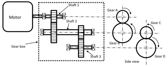
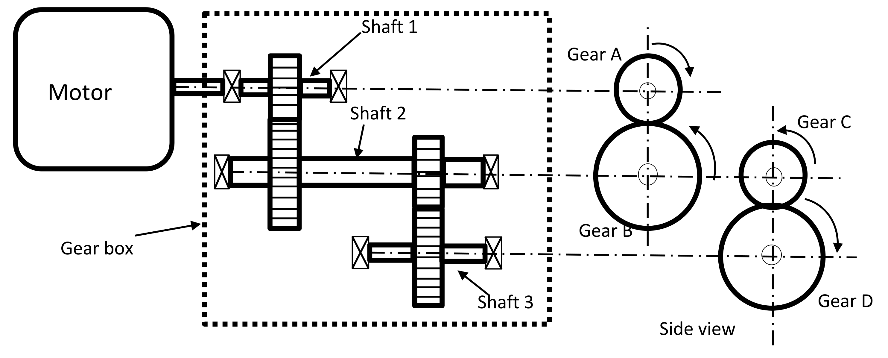
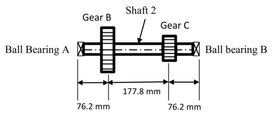
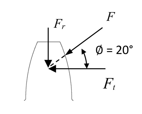
The application of the proposed method is based on the traditional design methodology. Therefore, the application is as shown in Figure 4. As an application, the intermediate shaft of the speed reducer is used to determine the principal stresses values that are acting on the ball bearing. Here, the speed is reduced from the initial 188 rad/s to a final speed of 47 rad/s. Initially, the motor transmits a constant power of 8.95 × 10⁶ N mm/s. Additionally, in the intermediate shaft and through the gears, the initial speed of 188 rad/s is reduced to 94 rad/s, while the power of 8.95 × 10⁶ N mm/s remains constant. The intermediate shaft is shown in Figure 5. This shaft is made of AISI 1020 steel with a shaft’s diameter (d_S) of 45 mm. The designed shaft will rotate with an angular speed of 94 rad/s. In addition, while the pass diameter of gear B is 127 mm, for gear C it is 76.2 mm. Moreover, the pression angle between these gears is 20°, as shown in Figure 6.

Figure 4. Speed reducer design connected to a motor.

Figure 5. Top view of shaft 2.

Figure 6. Gear’s pressure angle.

By having the dimensions of the selected bearing, the application of the Hertz theory is carried out to obtain the main stresses that are acting in the bearing outer race. This is done in order to use them for determining the Weibull distribution parameters that will allow us to determine the actual reliability of the ball bearing.

The step-by-step analysis given in Section 2.1 is as follows.

Step 0. The loads which are acting in shaft 2 are first determined. Since the torque generated on axis 2 depends on the angular speed (ω) of rotation and the power (P) that the axis transmits, then the constant torque generated on shaft 2 is:

$$T=\frac{P}{\omega }=\frac{8.95 \times {10}^6 \mathrm{N}·\mathrm{mm}/\mathrm{s}}{94\mathrm{rad}/\mathrm{s}}=\mathrm{95,212.76} \mathrm{N}·\mathrm{mm}$$

(36)

Additionally, since shaft 2 is in the equilibrium, then the generated torque in gears B and C is equal but in an opposite direction. Thus, torque in C is T_c = −95,212.76 N mm. On the other hand, as shown in Figure 6, the radial and tangential forces that are acting on the gears depend on the pression angle of Φ = 20°.

Therefore, in the function of the torque and convergence ratio, the tangential force is given by:

$$F_t=\frac{T}{r}$$

(37)

Then, the corresponding radial force is given by:

$$F_r=\left(F_t\right)\tan \varnothing$$

(38)

Additionally, since for gears B and C Φ = 20°, and r_B = 63.5 mm and r_C = 38.1 mm, then numerically:

$F_{tB}=\frac{T}{r_B}=\frac{\mathrm{95,212.76} \mathrm{N}·\mathrm{mm}}{63.5 \mathrm{mm}}=1500 \mathrm{N}$, and $F_{rB}=F_{tB}tan\varnothing =\left(1500 \mathrm{N}\right)\tan 20°=546 \mathrm{N}$$F_{tC}=\frac{T}{r_C}=\frac{\mathrm{95,212.76} \mathrm{N}·\mathrm{mm}}{38.1 \mathrm{mm}}=2500 \mathrm{N}$, and $F_{rC}=F_{rC}tan\varnothing =\left(2500 \mathrm{N}\right)\tan 20°=910 \mathrm{N}$.

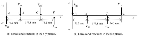
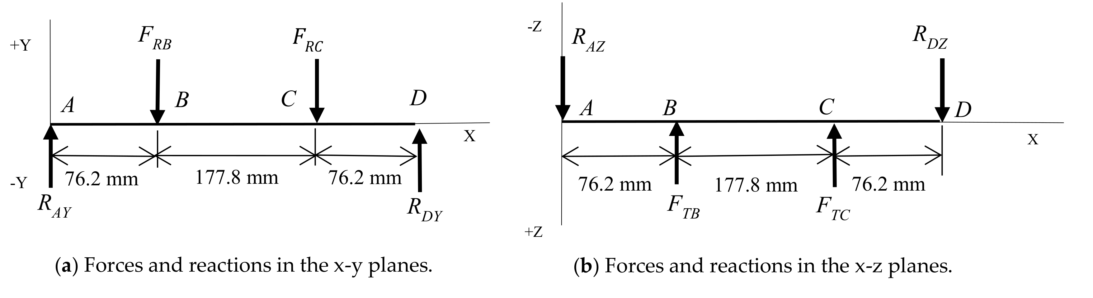
The radial and tangential forces, as well as the corresponding reactions that are acting in the x-y and in the x-z plane, are shown in Figure 7.

Figure 7. Forces and reactions in the x-y and x-z planes.

Thus, as shown in Figure 7a, the forces and reactions that are acting in the x-y plane are: $+\circlearrowleft \sum M_D=0=\left(910\mathrm{N}\right)\left(76.2\mathrm{mm}\right)+\left(546\mathrm{N}\right)\left(254\mathrm{mm}\right)-\left(330.2\mathrm{m}\right)\left(R_{Ay}\right);$ $R_{Ay}=630 \mathrm{N}$; $\sum F_y=0=630\mathrm{N}-546\mathrm{N}-910\mathrm{N}+R_{Dy};$ $R_{Dy}=826\mathrm{N}$.

Similarly, as shown in Figure 7b, the forces and reactions that are acting in the x-z plane are: $+\circlearrowleft \sum M_D=0=\left(R_{Az})(330.2\mathrm{mm}\right)-\left(1500\mathrm{N}\right)\left(254\mathrm{mm}\right)-\left(2500\mathrm{N}\right)\left(76.2\mathrm{mm}\right);$ $R_{Az}=1730\mathrm{N}$; $\sum F_z=0=-1730\mathrm{N}+1500\mathrm{N}+2500\mathrm{N}-R_{Dz}$; $R_{Dz}=2270\mathrm{N}$.

Therefore, the reaction forces in points A and D are:

$$R_A=\sqrt{R_{Ay}^2+R_{AZ}^2}=1841 \mathrm{N}$$

(39)

$$R_D=\sqrt{R_{Dy}^2+R_{DZ}^2}=2415.6 \mathrm{N}$$

(40)

Additionally, since $R_D>R_A$, then $R_D$ represents the reaction force value base on which the ball bearing is selected.

Step 1. Since we do not have an axial force for shaft 2, then from Equation (1) the design load is directly given by the radial force represented by $R_D$. Therefore, P = R_D = 2415.6 N. Additionally, since the inner race is the one that is rotating, then V = 1, and consequently, from Equation (2) the designed load is:

$$P_d=VP=\left(1\right)\left(2415.6\mathrm{N}\right)=2415.6\mathrm{N}$$

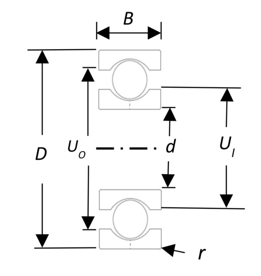
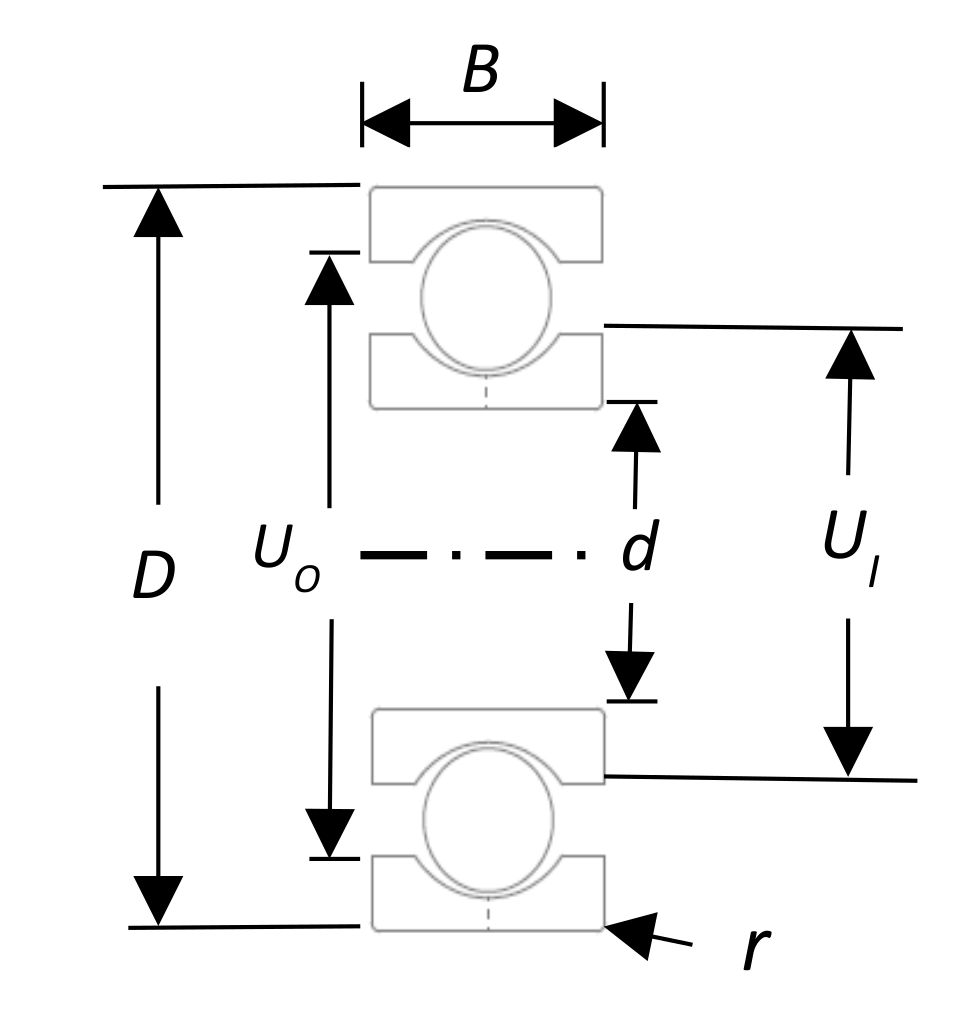
Step 2. Since from the design shaft phase, the diameter of shaft 2 is 45 mm, and from step 1 P_d = 2415.6 N, then from the SKF catalogue the selected ball bearing is the 6009 SKF type ball bearing with a bore diameter of 45 mm. The related ball bearing characteristics are given in Figure 8 and in Table 2.

Figure 8. Ball bearing dimensions.

Table 2. Ball bearing specifications.

Bearing Type	Capped Single Row Deep Groove Ball Bearings
Bore Diameter (d)	45 mm
Outer Diameter (D)	75 mm
Width (B)	16 mm
Dynamic Load Rating (C)	22,100 N
Static Load Rating (Co)	14,600 N
Max Speed	1047 rad/s
Max. Shaft Shoulder Dia. Inner (Ui)	67.8 mm
Min. Housing Shoulder Dia., Outer (Uo)	54.7 mm
Chamfer radius (r)	1 mm
Ball Quantity	13
Ball Diameter (db)	8.731 mm
Material	52,100 Chrome Steel

Step 3. According to the catalogues, the designed L₁₀ life of the ball bearing is:

$$L_{10}={10}^6{\left(\frac{\mathrm{22,100}\mathrm{N}}{2415.6\mathrm{N}}\right)}^3=765.77 \times {10}^6 \mathrm{rev}$$

With this data, the contact area generated in the ball bearing mentioned in Section 2.1 is determined as follows.

Step 4. Since the curvature generated in the x direction is $r_{ax}=r_{ay}=4.365 \mathrm{mm}$ and $r_{bx}=35.003125 \mathrm{mm}$, then $\frac{1}{R_x}=\frac{1}{4.365 \mathrm{mm}}-\frac{1}{35.003125 \mathrm{mm}}=0.20052 {\mathrm{mm}}^{-1}$, and therefore, $R_x=4.986 \mathrm{mm}$.

Additionally, since the outer ratio r_by is unknown, then from Equation (7) by using the compliance value of 0.52, the r_by value is $r_{by}=d{R}_r=\left(8.731\mathrm{mm}\right)\left(0.52\right)=4.54\mathrm{mm}$, therefore, $\frac{1}{R_y}=\frac{1}{4.365\mathrm{mm}}-\frac{1}{4.54\mathrm{mm}}=0.00883 {\mathrm{mm}}^{-1}$ implying $R_y=113.24 \mathrm{mm}.$ Moreover, since $\frac{1}{R}=0.20052 {\mathrm{mm}}^{-1}+0.00883 {\mathrm{mm}}^{-1}=0.20935 {\mathrm{mm}}^{-1}$, then the total curvature is $R=4.77 \mathrm{mm}$.

Step 5. From Equation (8), the curvature’s index α_r is:

$${\alpha }_r=\frac{113.24\mathrm{mm}}{4.986\mathrm{mm}}=22.7$$

Step 6. From Equation (9), the elliptical parameter k_e is:

$$k_e={\left(22.7\right)}^{\raisebox{1ex}{$2$}\!\left/ \!\raisebox{-1ex}{$\pi $}\right.}=7.3$$

Step 7. Since k_e < 100, the equations of Table 1 are selected.

Step 7.1. The simplified values of the first and second order elliptical equations $\mathcal{F}$ y $\mathcal{E}$ are:

$$\mathcal{F}=\frac{\pi }{2}+\left(\frac{\pi }{2}-1\right)\ln \left(22.7\right)=3.353$$

$$\mathcal{E}=1+\frac{\left(\frac{\pi }{2}-1\right)}{22.7}=1.025$$

Step 8. From Equation (10) by using the Poisson ratio of AISI 52100 v_a = v_b = 0.30 and its elasticity module E_a = E_b = 200 GPa of the material, the effective elasticity module is:

$$E^{\prime }=\frac{2}{\frac{[1-{\left(0.30\right)}^2]}{200\times {10}^9\mathrm{Pa}}+\frac{[1-{\left(0.30\right)}^2]}{200\times {10}^9\mathrm{Pa}}}=219.8\mathrm{GPa}$$

Step 9. Based on the diameter $D_y$ and $D_x$ of the ellipse formed in the contact area between the ball and the outer ring given in Equations (11) and (12), the a y b values of the axis are:

$$D_y=2{\left[\frac{6{\left(7.3\right)}^2\left(1.025\right)\left(2415.6\mathrm{N}\right)\left(4.77\mathrm{mm}\right)}{\pi (219,800\mathrm{N}/{\mathrm{mm}}^2)}\right]}^{\raisebox{1ex}{$1$}\!\left/ \!\raisebox{-1ex}{$3$}\right.}=3.52\mathrm{mm}$$

$$a=\frac{3.52 \mathrm{mm}}{2}=1.76 \mathrm{mm}$$

$$D_x=2{\left[\frac{6\left(1.025\right)\left(2415.6\mathrm{N}\right)\left(4.77\mathrm{mm}\right)}{\pi \left(7.3\right)(219,800\mathrm{N}/{\mathrm{mm}}^2)}\right]}^{\raisebox{1ex}{$1$}\!\left/ \!\raisebox{-1ex}{$3$}\right.}=0.48 \mathrm{mm}$$

$$b=\frac{0.48\mathrm{mm}}{2}=0.24\mathrm{mm}$$

Now, based on the above analysis, the contact principal stresses values mentioned in Section 2.3 are determined as follows.

Step 10. From Equation (13) the maximum stress P_max value is:

$$P_{max}=\frac{6\left(2415.6\mathrm{N}\right)}{\pi \left(3.52\mathrm{mm}\right)\left(0.48\mathrm{mm}\right)}=2713.5\mathrm{N}/{\mathrm{mm}}^2$$

Step 11. From Equations (14) to (17) the principal contact stresses σ_x, σ_y, σ_z, values, and the maximum shear τ_max value, as well as the depth at which τ_max occurs are as follows.

Step 11.1. From Equations (18) and (19) the k, k’ values are:

$$k=\frac{b}{a}=\frac{0.24\mathrm{mm}}{1.76\mathrm{mm}} =0.137$$

$$k^{\prime }=\sqrt{1-k^2}=\sqrt{1-{\left(0.137\right)}^2}=0.9905$$

Additionally, from Equation (20) the corresponding depth value is:

$$z=0.78 b=0.78\left(0.24\mathrm{mm}\right)=0.188 \mathrm{mm}$$

Step 11.2. From Equations (21) to (27) the n, M, Ω_x, Ω_y, Ω’_x, Ω’_y and Δ parameters used to determine the corresponding σ_x, σ_y y σ_z values are:

$$n=\sqrt{\frac{k^2+k^2{\left(\frac{z}{b}\right)}^2}{1+k^2{\left(\frac{z}{b}\right)}^2}}=\sqrt{\frac{{\left(0.137\right)}^2+{\left(0.137\right)}^2{\left(\frac{0.188 \mathrm{mm}}{0.24 \mathrm{mm}}\right)}^2}{1+{\left(0.137\right)}^2{\left(\frac{0.188 \mathrm{mm}}{0.24 \mathrm{mm}}\right)}^2}} = 0.172$$

$$M=\frac{2k}{{k^{\prime }}^2\mathcal{E}}=\frac{2\left(0.137\right)}{{\left(0.9905\right)}^2\left(1.025\right)}=0.2724$$

$${\mathsf{\Omega }}_x=-\frac{1-n}{2}+k\frac{z}{b}\left[\mathcal{F}-\mathcal{E}\right]$$

$${\mathsf{\Omega }}_x=-\left(\frac{1-0.172}{2}\right)+\left(0.137\right)\left(\frac{0.188 \mathrm{mm}}{0.24 \mathrm{mm}}\right)\left(3.353-1.025\right)$$

$${\mathsf{\Omega }}_x=-0.164$$

$${{\mathsf{\Omega }}^{\prime }}_x=-\frac{n}{k^2}+1+k\frac{z}{b}\left[\left(\frac{1}{k^2}\right)\mathcal{E}-\mathcal{F}\right]$$

$${{\mathsf{\Omega }}^{\prime }}_x=-[\frac{0.172}{{\left(0.137\right)}^2}]+1+0.137\left(\frac{0.18798}{0.24}\right)\left[[\frac{1}{{\left(0.137\right)}^2}]\left(1.025\right)-3.353\right]$$

$${{\mathsf{\Omega }}^{\prime }}_x=-2.72$$

$${\mathsf{\Omega }}_y=\frac{1}{2n}+\frac{1}{2}-\frac{n}{k^2}+k\frac{z}{b}\left[\left(\frac{1}{k^2}\right)\mathcal{E}-\mathcal{F}\right]$$

$${\mathsf{\Omega }}_y=\frac{1}{2\left(0.172\right)}+\frac{1}{2}-\frac{0.172}{{\left(0.137\right)}^2}+0.137\left(\frac{0.18798}{0.24}\right)\left[[\frac{1}{{\left(0.137\right)}^2}]\left(1.025\right)-3.353\right]$$

$${\mathsf{\Omega }}_y=-0.3286$$

$${{\mathsf{\Omega }}^{\prime }}_y=-1+n+k\frac{z}{b}\left(\mathcal{F}-\mathcal{E}\right)$$

$${{\mathsf{\Omega }}^{\prime }}_y=-1+0.172+0.137\left(\frac{0.18798}{0.24}\right)\left(3.353-1.025\right)$$

$${{\mathsf{\Omega }}^{\prime }}_y=-0.579$$

Step 11.3. From Equations (28) and (29) the A and B values to determine ∆ are:

$$A=\frac{1}{2}\left(\frac{1}{4.365\mathrm{mm}}+\frac{1}{-4.54\mathrm{mm}}\right)=4.415\times {10}^{-3} {\mathrm{mm}}^{-1}$$

$$B=\frac{1}{2}\left(\frac{1}{4.365\mathrm{mm}}+\frac{1}{-35.003125\mathrm{mm}}\right)=0.10026{\mathrm{mm}}^{-1}$$

Therefore, from Equation (27) the values are:

$$\Delta =\frac{1}{4.415\times {10}^{-3}{\mathrm{mm}}^{-1}+0.10026{\mathrm{mm}}^{-1}}\left[\frac{1-{\left(0.30\right)}^2}{\mathrm{200,000}\mathrm{N}/{\mathrm{mm}}^2}+\frac{1-{\left(0.30\right)}^2}{\mathrm{200,000}\mathrm{N}/{\mathrm{mm}}^2}\right]=8.6933\times {10}^{-5}{\mathrm{mm}}^3/\mathrm{N}$$

Then, from Equations (14) to (16) the principal contact stresses values are:

$${\sigma }_x=\left[\left[0.2724\left(-0.1648+\left(0.30\right)(-2.7238\right)\right]\left(\frac{0.24}{8.7\times {10}^{-5}}\right)\right]$$

$${\sigma }_x=-\mathrm{741,522,665.686} \mathrm{Pa}$$

$${\sigma }_y=\left[\left[0.2764\left(-0.3286+\left(0.30\right)(-0.5785\right)\right]\left(\frac{0.241}{8.7\times {10}^{-5}}\right)\right]$$

$${\sigma }_y=-\mathrm{384,772,372.51} \mathrm{Pa}$$

$${\sigma }_z=\left[-\left[\frac{0.2764}{2}\left(\frac{1}{0.1727}-0.1727\right)\right]\left(\frac{0.241}{8.6933\times {10}^{-5}}\right)\right]$$

$${\sigma }_z=-\mathrm{2,152,276,334.65} \mathrm{Pa}$$

Additionally, from Equation (17) the maximum shear stress value is:

$${\tau }_{máx}=\frac{\left(\mathrm{2,152,276,334.65}-\mathrm{384,772,372.51}\right)}{2}=\mathrm{883,751,981.07}\mathrm{Pa}$$

Now, based on the above stress values, the Weibull parameters used to determine the actual life and reliability of the ball bearing are determined, as mentioned in Section 2.4.

Step 12. Determine the Weibull η and β parameters. By using the maximum contact stress value σ₁ and minimum contact stress value in Equation (30), the use Weibull scale parameter is [22]:

$${\eta }_{use}=\sqrt{{\sigma }_1 {\sigma }_3}=\sqrt{\left(\mathrm{2,152,276,334.65}\right)\left(\mathrm{384,772,372.51}\right)}=\mathrm{910,020,039.1}$$

Additionally, from Equation (31) the Weibull shape parameter is:

$$\beta =-\frac{4{\mu }_y}{0.995ln\left(\frac{{\sigma }_1}{{\sigma }_3}\right)}=-\frac{4\left(-0.54562412\right)}{0.995\ln \left(\frac{\mathrm{2,152,276,334.65}}{\mathrm{384,772,372.51}}\right)}=1.274062\cong 1.27$$

Therefore, the Weibull parameters to determine the life of the ball bearing are W (1.28, 910,020,039.1 rev). With these parameters, the actual reliability of the ball bearing is as mentioned in Section 2.5.

Step 13a. From Equation (32) using the catalogues L₁₀ life of 765.77 × 10⁶ rev and the Weibull scale parameter, the reliability of the ball bearing is estimated to be:

$$R\left(t\right)=\exp \left\{-{\left(\frac{L_{10}}{{\eta }_{use}}\right)}^{\beta }\right\}=\exp \left\{-{\left(\frac{765.77\times {10}^6}{\mathrm{910,020,039.1}}\right)}^{1.28}\right\}=0.4485$$

At this point, it is very important to note that the used L₁₀ value does not represent the applied stress, (it represents the expected life at the conditions at which the ball bearing was designed). In addition, the η_use value does not represent the strength conditions at which the ball bearing was designed. Therefore, the estimated reliability of R(t) = 0.4485 does not represent the life that corresponds to the actual environment at which shaft 2 operates. Therefore, to determine the actual reliability we must proceed with the next steps.

Step 13b. By setting Equation (32) at R(t) = 0.90, the actual L_10(use) life that represents the actual conditions at which shaft 2 operates is given from Equation (33) as $L_{10\left(use\right)}={\eta }_{use}\left(\sqrt[\beta ]{-\ln \left(0.90\right)}\right)=\mathrm{156,862,111.04}rev$.

Now that the L_10(use) value represents the environmental actual stress, it is necessary to determine the Weibull scale parameter that represents the strength of the selected ball bearing. It is determined as follows.

Step 13c. The catalogues strength η_cat value that represents the strength of the ball bearing is determined from Equation (34) using the catalogue L₁₀ life. It is η_cat = $\frac{L_{10}}{\sqrt[\beta ]{-\ln \left(0.90\right)}}$ = 4,442,538,996.4 rev.

Finally, using the $L_{10\left(use\right)}$ value and the η_cat value, the actual reliability is as follows.

Step 13d. From Equation (32) the actual reliability of the selected ball bearing is:

$$R\left(t\right)=\exp \left\{-{\left(\frac{L_{10\left(use\right)}}{\eta cat}\right)}^{\beta }\right\}=\exp \left\{-{\left(\frac{\mathrm{15,686,211.04}}{\mathrm{4,442,538,996.4}}\right)}^{1.28}\right\}=0.9992$$

Finally, in step 13d, the actual reliability of the ball bearing is higher than the designed reliability of R(t) = 0.90. In addition, this occurs mainly since the estimated $L_{10\left(use\right)}$ life is lower than the catalogues $L_{10}$ life ($L_{10\left(use\right)}<L_{10})$. The actual reliability resulting in the ball bearing is greater than the reliability of the life equation L₁₀ offered by the manufacturer due to the fact that it was analyzed with different loads than those used by the manufacturer. Since the actual reliability is different, it can be said that this methodology can be used to obtain the reliability in cases where the bearing is subjected to different load magnitudes and is required to know its current reliability.

4. Conclusions

• The environment in which the catalog life of ball bearings is determined does not correspond to its use in practice.
• Based on the contact stresses generated between the ball and the race, the proposed method allows us to determine the current life of the ball bearing, which represents the conditions of use.
• In determining the current reliability of the ball bearing, the Weibull distribution of two parameters is used where the parameters are directly determined from the contact stresses.
• The efficiency of the method to determine the life of the ball bearing is based on the fact that the catalog η value represents the resistance of the ball bearing material.
• The proposed method can be applied to determine the reliability for different bearing applications.

References

- Yu, J.; Ding, B.; He, Y. Rolling bearing fault diagnosis based on mean multigranulation decision-theoretic rough set and non-naive Bayesian classifier. J. Mech. Sci. Technol. 2018, 32, 5201–5211. [Google Scholar] [CrossRef] [Scilit]
- Panda, S.; Panda, S.N.; Nanda, P.; Mishra, D. Comparative study on optimum design of rolling element bearing. Tribol. Int. 2015, 92, 595–604. [Google Scholar] [CrossRef] [Scilit]
- Upadhyay, N.; Kankar, P.K. Diagnosis of bearing defects using tunable Q-wavelet transform. J. Mech. Sci. Technol. 2018, 32, 549–558. [Google Scholar] [CrossRef] [Scilit]
- Yakout, M.; Nassef, M.G.A.; Backar, S. Effect of clearances in rolling element bearings on their dynamic performance, quality and operating life. J. Mech. Sci. Technol. 2019, 33, 2037–2042. [Google Scholar] [CrossRef] [Scilit]
- Guo, W.; Cao, H.; He, Z.; Yang, L. Fatigue Life Analysis of Rolling Bearings Based on Quasistatic Modeling. Shock Vib. 2015, 2015. [Google Scholar] [CrossRef] [Scilit]
- Budynas, R.G.; Nisbett, K. Shigley’s Mechanical Enginering Desing, 10th ed.; McGraw-Hill Education: Pennsylvania, NY, USA, 2015. [Google Scholar]
- Oswald, F.B.; Zaretsky, E.V. Comparison of Models for Ball Bearing Dynamic Capacity and Life. Tribol. Trans. 2018, 58, 1039–1053. [Google Scholar]
- Zaretsky, E.V. Rolling bearing life prediction, theory, and application. In NASA Technical Reports; NASA: Washington, USA, 2013; pp. 1–54. [Google Scholar]
- Zaretsky, E.V. A. Palmgren revisited-A basis for bearing life prediction. Lubr. Eng. 1998, 54, 18–23. [Google Scholar]
- Oswald, F.B.; Zaretsky, E.V.; Poplawski, J.V. Interference-fit life factors for ball bearings. Tribol. Trans. 2011, 54, 1–20. [Google Scholar] [CrossRef] [Scilit]
- Zaretsky, E.V. In search of a fatigue limit: A critique of ISO Standard 281:2007. Tribol. Lubr. Technol. 2010, 66, 30–40. [Google Scholar]
- Hamrock, B.J.; Dowson, D. Ball Bearing Mechanics. In NASA Technical Memorandum; NASA: Washington, DC, USA, 1981; pp. 1–106. [Google Scholar]
- Aucktor, E.; Schmltz, F.; Seherr-Toss, H.C. Universal Joints and Driveshafts; Springer: Berlin, Germany, 1992. [Google Scholar]
- Anoopnath, P.R.; Babu, V.S.; Vishwanath, A.K. Hertz Contact Stress of Deep Groove Ball Bearing. Mater. Today Proc. 2018, 5, 3283–3288. [Google Scholar] [CrossRef] [Scilit]
- Hertz, H. Ueber die Berührung fester elastischer Körper. J. Reine Angew. Math. 1882, 92, 156–171. [Google Scholar]
- Herák, D.; Chotěborský, R.; Sedláček, A.; Janča, E. Exploitation of Hertz’s contact pressures in friction drives. Res. Agric. Eng. 2012, 52, 107–113. [Google Scholar] [CrossRef] [Scilit]
- International Organization for Standardization. ISO 281:2007(E), Rolling Bearings—Dynamic Load Ratings and Rating Life, 2nd ed.; International Organization for Standardization: Geneva, Switzerland, 2007. [Google Scholar]
- Adeshara, D.; Darji, P. A Review of Design and Analysis of Angular Contact Ball Bearing for Two Wheeler Clutch. Int. J. Adv. Eng. Res. Dev. 2015, 2, 876–880. [Google Scholar] [CrossRef] [Scilit]
- Li, X.; Yu, K.; Ma, H.; Cao, L.; Luo, Z.; Li, H.; Che, L. Analysis of varying contact angles and load distributions in defective angular contact ball bearing. Eng. Fail. Anal. 2018, 91, 449–464. [Google Scholar] [CrossRef] [Scilit]
- Tong, V.C.; Hong, S.W. Statistical investigation into the effects of distributed roller diameter error on the fatigue life of tapered roller bearings. J. Mech. Sci. Technol. 2017, 31, 5977–5985. [Google Scholar] [CrossRef] [Scilit]
- Wagner, E.R.; Cooney, C.E. Universal Joint and Driveshaft Desing Manual, SAE AE-7, 1st ed.; Society of Automotive Engineers: Warrendale, PA, USA, 1979. [Google Scholar]
- Piña-Monarrez, M.R. Weibull stress distribution for static mechanical stress and its stress/strength analysis. Qual. Reliab. Eng. Int. 2018, 34, 229–244. [Google Scholar] [CrossRef] [Scilit]
Publisher’s Note: MDPI stays neutral with regard to jurisdictional claims in published maps and institutional affiliations. |
© 2020 by the authors. Licensee MDPI, Basel, Switzerland. This article is an open access article distributed under the terms and conditions of the Creative Commons Attribution (CC BY) license (http://creativecommons.org/licenses/by/4.0/).