Automatic Detection of Welding Defects Using Faster R-CNN


1
Department of Naval Architecture and Ocean Engineering, Pusan National University, Busan 46241, Korea
2
Department of Naval Vessel Service, Korean Register, Busan 46241, Korea
*
Author to whom correspondence should be addressed.
Appl. Sci. 2020, 10(23), 8629; https://doi.org/10.3390/app10238629
Submission received: 30 October 2020
/
Revised: 30 November 2020
/
Accepted: 1 December 2020
/
Published: 2 December 2020
(This article belongs to the Special Issue Nondestructive Testing (NDT): Volume II)
Abstract
:In the shipbuilding industry, the non-destructive testing for welding quality inspection is mainly used for the permanent storage of the testing results and the radio-graphic testing which can visually inspect the interior of the welded part. Experts are required to properly detect the test results and it takes a lot of time and cost to manually Interpret the radio-graphic testing image of the structure over 500 blocks. The algorithms that automatically interpret the existing radio-graphic testing images to extract features through image pre-processing and classify the defects using neural networks, and only partial automation is performed. In order to implement the feature extraction and classification in one algorithm and to implement the overall automation, this paper proposes a method of automatically detecting welding defect using Faster R-CNN which is a deep learning basis. We analyzed the data to learn algorithms and compared the performance improvements using data augmentation method to artificially increase the limited data. In order to appropriately extract the features of the radio-graphic testing image, two internal feature extractors of Faster R-CNN were selected, compared, and performance evaluation was performed.
1. Introduction
The welding process accounts for more than 60% of the entire process in the shipbuilding and offshore sector [1]. For the weld testing, there are various technologies such as radiographic testing (RT), ultrasonic testing (UT) and magnetic testing (MT) used as non-destructive testing (NDT). Of them, ship owners particularly prefer RT whose results can be stored permanently and that can visually check the inside of the weld of all materials to other types of NDT.
Currently, technicians directly perform welding testing on structures of 500 blocks or more to inspect the welding process in domestic and overseas shipyards. Since welding information of more than 2000 locations per block is manually prepared, omissions and errors commonly occur, which requires additional work, resulting in a huge amount of time and cost. To derive a consistent and rational result from testing that is manually conducted, there is a need for an automation and objectification system of testing that improves inspectors’ understanding.
Studies on automatic detection of the welding defects have been long conducted. Of them, ref. [2] used image pre-processing as a method of extracting features, and classified the type of welding defects using a neural network or Support Vector Machine (SVM) [3] for automatic identification. The form of the neural network used here is multi-layer perceptron (MLP) that is used only for classifying defects. Hence, it is not regarded as a neural network that classifies and reads images. Of various deep learning algorithms, a convolutional neural network (CNN) that has recently been researched a lot for image classification shows high performance compared to conventional algorithms. With regard to object detection, ref. [4] used CNN that achieved higher performance than previously used HOG [5] or SIFT [6]. In [7] the boundaries of defects were classified based on image feature map extracted from the neural network using CNN and SVM, but not only the boundaries of defects but also the types of defects are important because NDT rules depending on the type of defect. Among the methods of object detection using neural networks, Fast R-CNN [8] and Faster R-CNN [9] are mainly used for object detection as they can classify the types and locations of objects in one network. In the medical sector that handles radiographic images, research on object detection employing CNN has already been underway. CNN detected features different to normal ones in chest radiographic images [10], and a study was conducted to detect nerve regions using CNN in ultrasound images [11]. The performance of detecting objects in radiographic images can be confirmed in several studies, and the possibility of detecting defects in radiographic images using CNN was confirmed.
In this paper, we propose an algorithm that automatically detects the welding defects in radiographic images by employing Faster R-CNN that shows high-performance in terms of accuracy. We compared ResNet [12] and Inception-ResNet V2 [13] that showed high-performance in ImageNet by configuring them as backbone networks. We conducted an experiment by analyzing the anchor size in Faster R-CNN in a form suitable for defects. By taking into account the limited number of data, we improved the accuracy of the proposed algorithm using data augmentation. |Table 1 describes the method and features of defect detection.
2. Methodology
2.1. Convolutional Neural Network
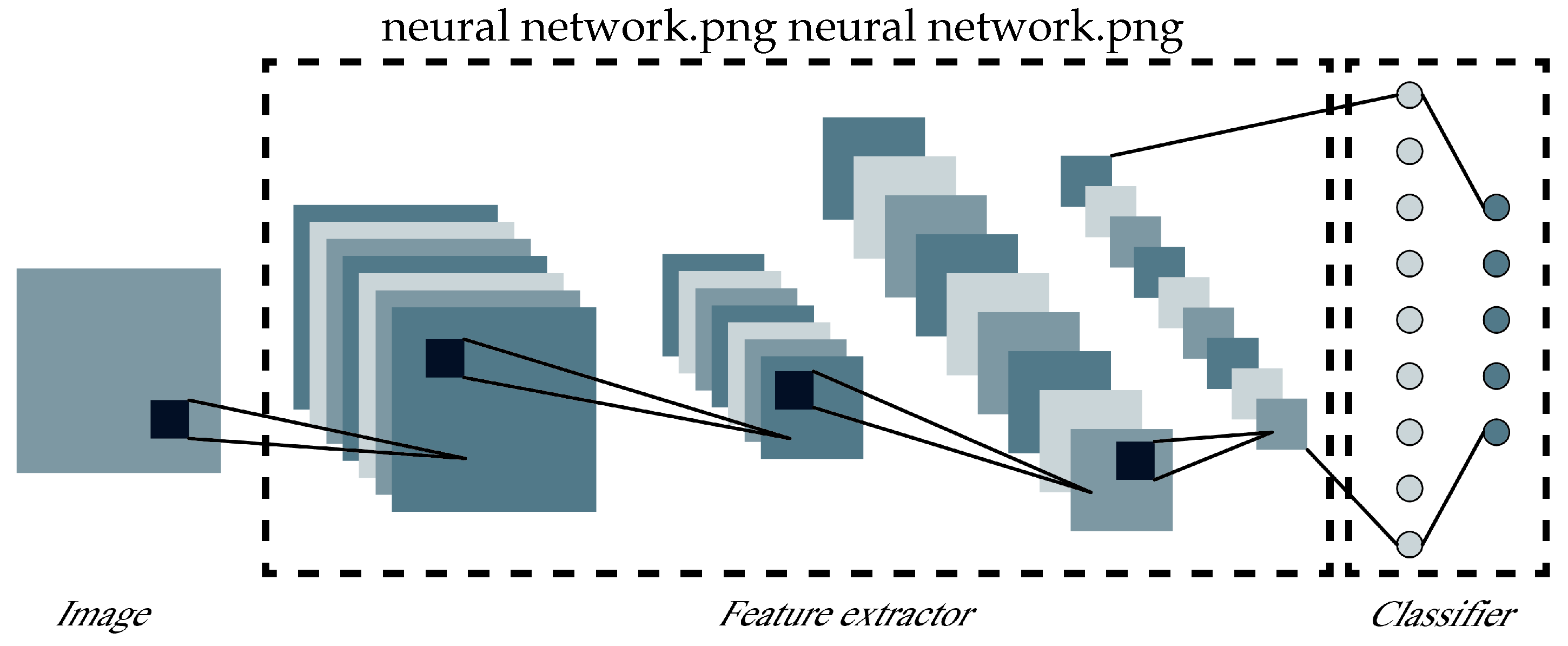
It is a technology that mimics the structure of the optic nerve, and automatically learns features necessary for the recognition of characters, images, objects, etc., starting from image processing. Unlike conventional algorithms, CNN does not require a separate image pre-processing step because it includes the feature extraction step. Further, various methods used when training a general neural network can be applied to CNN in the same way. It learns the classification process by repeating it multiples times to respond to various cases, thus resulting in high accuracy. A general CNN structure consists of convolutional layers, pooling layers, fully-connected layers, and Softmax (Figure 1). The convolutional layer corresponding to the feature extractor is composed of learnable filters. In each filter, the region connected to the input volume is stacked into a depth dimension called an activation map through the dot product of scalar multiples by element, and the stacked activation maps become output volumes. After this, the size of the input volume is readjusted by extracting representative values within a pixel unit of a certain size through the pooling layer. By stacking these configurations in multiple layers, the features of an image are extracted and filters are learned.
To apply a feature map extracted from the feature extractor composed of the convolution layer and the pooling layer to a classifier, 3D data is arranged and used as 1D data. The classifier consists of the fully-connected layer and Softmax, which are the form of a conventional neural network. By repeatedly training the fully-connected layer and Softmax along with the feature extractor, it ultimately classifies which class an image belongs to. As for classification problems in general CNN, only classes should be classified. However, class classification and location should be found when there is an object, thus information about location should also be learned.
2.2. Faster R-CNN
R-CNN is an object detection algorithm based on CNN. In classifying an object while searching all regions of an image with a filter of a certain size, it detects an object by learning region proposals that are the ranges where the object is likely to be using CNN. Faster R-CNN, as shown in Figure 2a, proposed a novel method by constructing a neural network in the conventional selective search as a method of obtaining region proposals. This neural network is referred to as a region proposal network (RPN), and learning is possible because the convolutional layer and fully-connected layer are configured. In addition, as it can use GPU operation, fast calculation is possible. RPN (Figure 2b) creates intermediate layers through sliding window by receiving 256 or 512 dimensions from the feature extractor. After this, it performs convolution with the classifier layer and regressor layer. The classifier layer obtains outputs by applying a 1 × 1 filter. This layer creates an anchor box with k different sizes and ratios generated for each sliding window, and assigns two scores, which indicates the existence of an object. The regressor layer also applies a 1 × 1 filter, creates k anchor boxes, and then assigns four coordinate values to indicate the coordinates of the bounding box. Learning is performed by inputting the outputs from the two layers into the fully-connected layer through the region of interest (RoI) pooling layer. By introducing RPN and the RoI pooling layer, Faster R-CNN addresses the computational and structural issues of R-CNN and fast R-CNN, and greatly improves accuracy and computation speed.
Faster R-CNN constructed with RPN can be backpropagated end-to-end, thus has fewer errors than before. In addition, from a structural perspective, as RPN can be implemented with the convolutional layer, it can be constructed coupled with the feature extractor. Thus, performance can be improved by applying several CNN structures that achieve high results in ImageNet.
2.3. ResNet
In forming a deep network, the gradient value becomes too large or saturated with small values, resulting in a vanishing gradient problem that loses or slows the learning effect. ResNet added an identity shortcut connection to the conventional neural network structure to obtain the learning effect of the deep network. As the shortcut connection that connects the input to the output is directly connected without parameters, only addition is added in terms of computation. Thus, it does not significantly influence the computation amount. Deep networks can be easily optimized using this, and accuracy can be improved due to the increased depth. Figure 3a shows the block of residual learning that composes ResNet [12]. Previously, was learned, but residual learning learns to obtain . This modified method in this way learns in a direction where should be 0, thus it is possible to easily detect movements with small inputs.
2.4. Inception-ResNet V2
Inception-ResNet is a model that combines structural features and is divided into V1 and V2. V1 refers to a model that combines Inception V3 and ResNet, and V2 is a model that combines Inception V4 and ResNet. Figure 3b shows the module A of Inception-ResNet [13]. It is similar to the form in the Inception module, however, as the reduction module was used, pooling disappeared and the concept of x identity in ResNet was introduced. The module form of Inception-ResNet V1 and Inception-ResNet V2 are the same, but there are differences in the number of internal filters and the modification of stem. The combined models have fast convergence speed compared to a single model. The Inception-ResNet model improves performance due to the difference between Inception V3 and V4. The high recognition rate and learning rate are verified through recent studies, and it is expected to achieve high outcomes when used as the feature extractor of the welding defect detection algorithm.
3. Welding Defect Data
We compared two feature extractors to evaluate the performance, and applied data augmentation to maximize the efficiency of a relatively small dataset. In the dataset, the defect types are composed of porosity, lacks of fusion, slag, and cracks, but the labeling for each type is biased toward porosity. Figure 4a shows the porosity, the most common defect type, with 569 defects included in the dataset. Lack of fusion and slag shown in Figure 4b,c are similar in shape and the amount of data for each class is small, thus they are grouped into a single defect that is classified as LoS (Lack or Slag). For the LoS, 236 defects are included in the dataset. After learning, there are two classes classified by the algorithm, that is, the porosity and LoS. The dataset is composed of radiographic testing images taken differently depending on the steel plate, pipe, and pipe size, thus it can be read and evaluated without dividing the weld after learning. The radiographic testing image of the weld of the pipe is composed of a relatively small pixel size by removing the background on both sides as well as the upper and lower base materials.
3.1. Pre-Processing
The pixel size of the images that make up the dataset is approximately 4900 × 1200 or higher, which is high quality. High-definition images degrade the learning rate, and it is difficult to expect good performance with an increase in the number of parameters to learn. To classify and read the taken image of the weld using radiographic testing, the information about the relevant radiographic image is marked on the base material. To remove noise arising from defects in the base metal or film, we removed the rest except for the weld and used it as the training data along with the information marked. Although noise is removed from the radiographic testing image, the longitudinal direction is maintained at a pixel size of 4900 or higher. Thus, it is necessary to reduce the size of the image by taking account of the learning rate and learning environment. In this study, we segmented the radiographic testing images to fit the weld into Section 2, Section 3, Section 4 and Section 5 (Figure 5). The segmented image becomes smaller from 4900 pixels to less than 980 pixels, and the learning rate was reduced from 1.7 s to 0.3 s per epoch. Most cracks or slag are present in the longitudinal direction of the weld. These defects were segmented by the segmented image, thus an increased effect could be obtained from the relevant defect data. The total number of data increased to 341 from the 134 through image segmentation. Of them, there are 321 training data and 20 validation data.
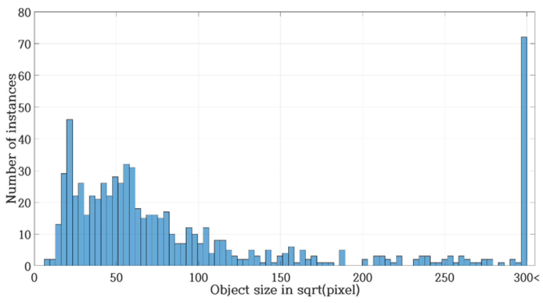
3.2. Small Object in Faster R-CNN
As a result of labeling and then measuring the size of defects appearing in the weld, as shown in Figure 6, the porosity is made up of the size of 10 to 40 pixels, and defects classified as the LoS, 340 pixels in the longitudinal direction. In MS COCO object detection competition [14], small (Area < ), medium ( < Area < ), and large ( < Area) are classified according to the pixel area, so the welds belong to both small and large object. We modified the size of the anchor box and the number of region proposal recommendations among the hyper parameters of Faster R-CNN to effectively detect the welding defects. To theoretically estimate the size of the anchor box generated in RPN, we selected the size and aspect ratio by taking into account intersection over union (IoU) according to [15].
In PASCAL VOC, regions where IoU is 0.5 or more are determined as true positive in Table 2 [16]. IoU is the ratio of the overlapped region between the labeled region and the estimated region, and is defined as:
represents the length of the labeled region (ground truth) and represents the length of the estimated region. d is the distance between the two regions, and is generated in longitudinal and vertical directions when the IoU is the lowest. Since IoU ≥ 0.5 should be valid, . Expressing Equation (1) for :
The threshold t is 0.5, and d is 8 since it is set as stride in the convolutional layer. For the relationship between and , an appropriate size of the anchor box is selected by considering according to [16]. By taking into account the pixel size of the LoS as well as the porosity, we set the size of the anchor box to be used in the experiment to 10, 40 and 80 pixels, and a total of 3 aspect ratios, which are 1:1, 1:5 and 5:1, to be suitable for the LoS.
4. Experiments and Results
We trained ResNet and Inception-ResNet V2 that were to be compared using the training data. After applying data augmentation to each algorithm, we evaluated a total of four things by training them one more time. During the training process, by analyzing the convergence of the loss values for the training data and the mean Average Precision(mAP) of the algorithm for the evaluation data, we designated the point at which the mAP for the evaluation data was highest as the end point. The detection rate-recall graph of the algorithms for the porosity and LoS is shown in Figure 7, respectively.
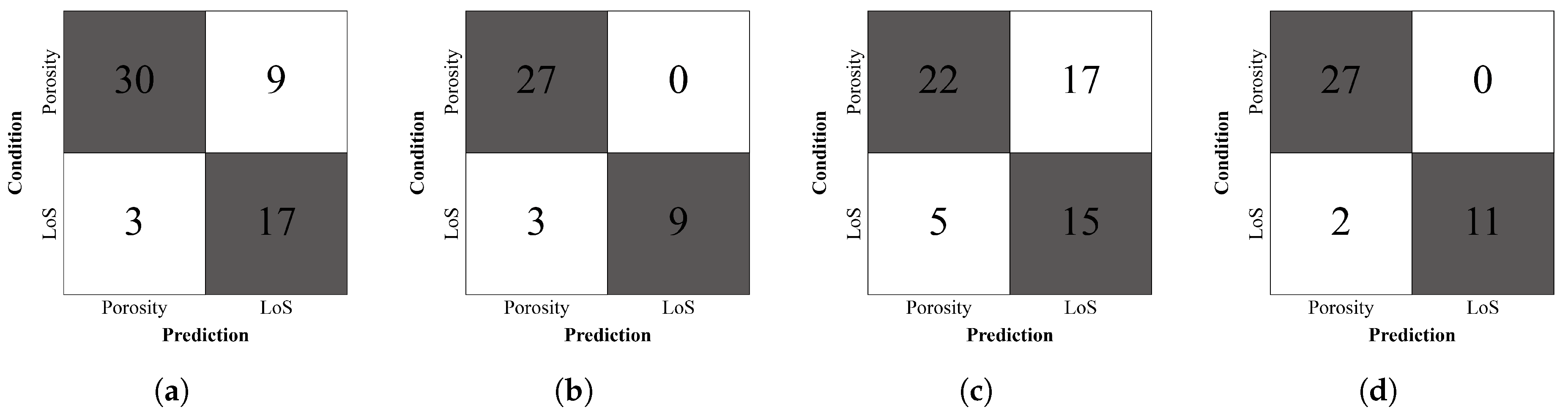
Table 3 shows the result of evaluating the performance of the algorithm. Overall, the detection rate of the LoS was significantly lower than that of the porosity, and 0.265 was measured as the highest performance in the algorithm that applied data conversion to ResNet. When comparing the feature extractor, ResNet showed relatively higher performance than Inception-ResNet V2. The difference was approximately 0.2 before data conversion was applied while the difference was approximately 0.27 after data conversion. The results of applying data conversion to the two algorithms that were to be compared showed higher performance than before applying it. When applying it to Inception-ResNet V2, the performance improved by approximately 0.008, and for ResNet, it improved by approximately 0.074. In contrast, the classification of confusion matrix based on the value of IoU > 0.5 as shown in Figure 8, more classification errors in the ResNet than Inception-ResNet V2. This shows that the classification of defect classes is lower than that of other models, but the performance of locations is better.
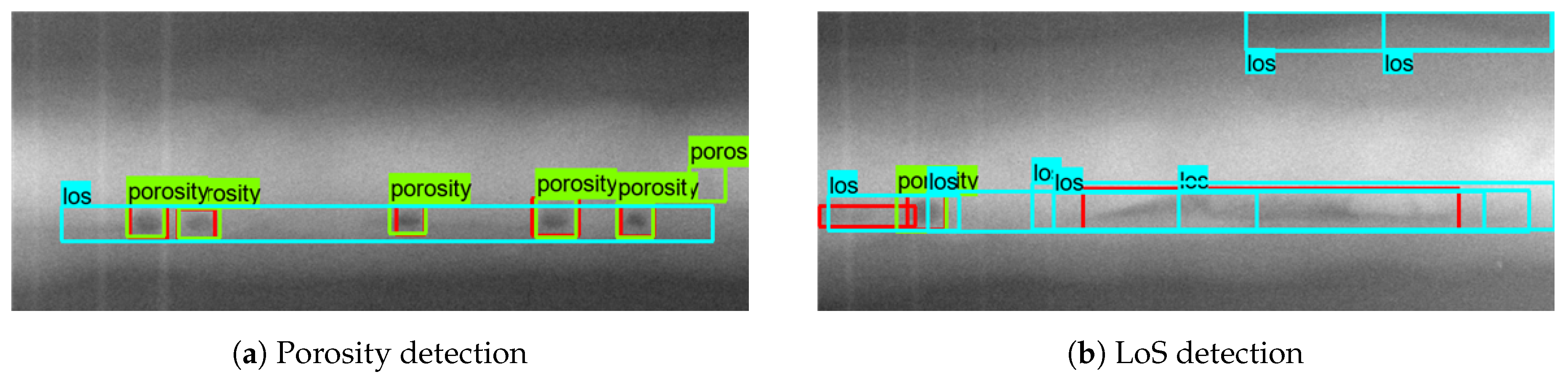
The welding defect detection results show that, for the welding defects occurring in the edge of the weld as seen in Figure 9a or in the longitudinal direction as seen in Figure 9b, the LoS welding defect detection do not operate normally. The porosity has similar training and evaluation data, and has a high overall detection rate. As the results labeled by expert opinions do not contain film defects, the circular defects shown in the evaluation data are not generated as data, thus resulting in performance degradation.
5. Conclusions
In this study, as the size of defects belonged to an object that was smaller than the size of existing objects, we set the size of the anchor box and aspect ratio to be suitable for small objects, and set the number of region proposal recommendations through an experiment. As the algorithms to be used in the experiment, we compared ResNet and Inception-ResNet V2 with the feature extractor of Faster R-CNN, and proposed ResNet with the highest performance. Because of the characteristics of shipyard radiographic testing, data is limited and the number of images that can be secured for each type of defect is extremely small. Therefore, data conversion is an essential element in the automatic welding defect detection algorithm. In this study, we used data conversion for efficient training and performance improvement. The experimental results show that data conversion could increase the performance by 0.074 in radiographic testing images. As the types of defects that actually occurred in the field were limited, we did not cover all of the welding defects when constructing a dataset, but covered specific welding defects to increase practicality. We analyzed the dataset and then divided it into the porosity and LoS, but the learning performance was different because the number of defects for each image varied. For the porosity, 569 defects were learned but for LoS, 236 defects were learned, thus leading to a result that was biased toward the porosity. We increased the data of the LoS through data conversion and image segmentation, but could not significantly decrease the biased results.
In this study, we used 321 radiographic testing images, and we will improve the accuracy of the algorithm by securing additional images in the future. In addition, by applying the actual defect reading application regulations, we will revise the pass and fail as the final result, and link the algorithm with welding testing automation. By newly setting the structure of the algorithm based on additional research, we will construct it to be suitable for the welding defects. Further, by taking into account various other defects as well as two defects covered in this study, we will expand the application range of the algorithm to automatically detect defects occurring in other industries other than the shipbuilding industry.
Author Contributions
Conceptualization, S.-j.O.; methodology, S.-j.O.; validation, C.L. and M.-j.J.; formal analysis, M.-j.J.; investigation, S.-j.O.; resources, C.L. and M.-j.J.; data curation, M.-j.J.; writing—original draft preparation, S.-j.O.; writing—review and editing, S.-c.S.; visualization, S.-j.O.; supervision, S.-c.S.; project administration, S.-c.S.; funding acquisition, S.-c.S. All authors have read and agreed to the published version of the manuscript.
Funding
This research received no external funding.
Acknowledgments
This work was supported by the Technology Innovation Program (20000252, Development of automatic inspection for welding quality based on AI with integrated management platform in shipbuilding and maritime domain) funded By the Ministry of Trade, Industry and Energy (MOTIE, Korea). This work was supported by the National Research Foundation of Korea(NRF) grant funded by the Korea government(MSIT) through GCRC-SOP (No. 2011-0030013). This work was supported by the Development of Autonomous Ship Technology(20200615, Development of remote management and safe operating technology of autonomous navigation system) funded by the Ministry of Oceans and Fisheries, Korea.
Conflicts of Interest
The authors declare no conflict of interest.
References
- Kim, Y.; Kim, J.; Kang, S. A Study on Welding Deformation Prediction for Ship Blocks Using the Equivalent Strain Method Based on Inherent Strain. Appl. Sci. 2019, 9, 4906. [Google Scholar] [CrossRef] [Green Version]
- Vilar, R.; Zapata, J.; Ruiz, R. An automatic system of classification of weld defects in radiographic images. Ndt Int. 2009, 42, 467–476. [Google Scholar] [CrossRef]
- Martínez, J.; Iglesias, C.; Matías, J.M.; Taboada, J.; Araújo, M. Solving the slate tile classification problem using a DAGSVM multiclassification algorithm based on SVM binary classifiers with a one-versus-all approach. Appl. Math. Comput. 2014, 230, 464–472. [Google Scholar] [CrossRef]
- Girshick, R.; Donahue, J.; Darrell, T.; Malik, J. Rich feature hierarchies for accurate object detection and semantic segmentation. In Proceedings of the IEEE Conference on Computer Vision and Pattern Recognition, Columbus, OH, USA, 23–28 June 2014; pp. 580–587. [Google Scholar]
- Dalal, N.; Triggs, B. Histograms of oriented gradients for human detection. In Proceedings of the 2005 IEEE Computer Society Conference on Computer Vision and Pattern Recognition (CVPR’05), San Diego, CA, USA, 20–25 June 2005; Volume 1, pp. 886–893. [Google Scholar]
- Lowe, D.G. Distinctive image features from scale-invariant keypoints. Int. J. Comput. Vis. 2004, 60, 91–110. [Google Scholar] [CrossRef]
- Sizyakin, R.; Voronin, V.; Gapon, N.; Zelensky, A.; Pižurica, A. Automatic detection of welding defects using the convolutional neural network. Autom. Vis. Insp. Mach. Vis. III 2019, 11061, 110610E. [Google Scholar]
- Girshick, R. Fast r-cnn. In Proceedings of the IEEE International Conference on Computer Vision, Santiago, Chile, 7–13 December 2015; pp. 1440–1448. [Google Scholar]
- Ren, S.; He, K.; Girshick, R.; Sun, J. Faster r-cnn: Towards real-time object detection with region proposal networks. In Proceedings of the Advances in Neural Information Processing Systems, Montreal, QC, Canada, 7–12 December 2015; pp. 91–99. [Google Scholar]
- Tang, Y.X.; Tang, Y.B.; Peng, Y.; Yan, K.; Bagheri, M.; Redd, B.A.; Brandon, C.J.; Lu, Z.; Han, M.; Xiao, J.; et al. Automated abnormality classification of chest radiographs using deep convolutional neural networks. NPJ Digit. Med. 2020, 3, 1–8. [Google Scholar] [CrossRef]
- Hafiane, A.; Vieyres, P.; Delbos, A. Deep learning with spatiotemporal consistency for nerve segmentation in ultrasound images. arXiv 2017, arXiv:1706.05870. [Google Scholar]
- He, K.; Zhang, X.; Ren, S.; Sun, J. Deep residual learning for image recognition. In Proceedings of the IEEE Conference on Computer Vision and Pattern Recognition, Las Vegas, NV, USA, 26 June–1 July 2016; pp. 770–778. [Google Scholar]
- Szegedy, C.; Ioffe, S.; Vanhoucke, V.; Alemi, A. Inception-v4, inception-resnet and the impact of residual connections on learning. arXiv 2016, arXiv:1602.07261. [Google Scholar]
- Lin, T.Y.; Maire, M.; Belongie, S.; Hays, J.; Perona, P.; Ramanan, D.; Dollár, P.; Zitnick, C.L. Microsoft coco: Common objects in context. In Proceedings of the European Conference on Computer Vision, Zurich, Switzerland, 6–12 September 2014; pp. 740–755. [Google Scholar]
- Kisantal, M.; Wojna, Z.; Murawski, J.; Naruniec, J.; Cho, K. Augmentation for small object detection. arXiv 2019, arXiv:1902.07296. [Google Scholar]
- Everingham, M.; Van Gool, L.; Williams, C.K.; Winn, J.; Zisserman, A. The pascal visual object classes (voc) challenge. Int. J. Comput. Vis. 2010, 88, 303–338. [Google Scholar] [CrossRef] [Green Version]
Figure 1.
General CNN structure. Consisted to feature extractor and classifier.

Figure 2.
(a) Faster R-CNN structure. (b) RPN takes an image as input and outputs a set of rectangular object proposals, each with an objectness score.
Figure 2.
(a) Faster R-CNN structure. (b) RPN takes an image as input and outputs a set of rectangular object proposals, each with an objectness score.

Figure 3.
(a) Module learned to converge H(x) − x to zero. (b) 1 × 1 convolutions are used to compute reductions before the expensive 3 × 3 and 5 × 5 convolutions.
Figure 3.
(a) Module learned to converge H(x) − x to zero. (b) 1 × 1 convolutions are used to compute reductions before the expensive 3 × 3 and 5 × 5 convolutions.

Figure 4.
Welding defect.

Figure 5.
Divided radio-graphic testing image.

Figure 6.
Number of instances and defect size (pixel).

Figure 7.
Precision-recall curve. Calculate the average precision of porosity and loss according to PASCAL VOC [16] criteria. The solid line represents porosity, and the dotted line represents LoS for each model.
Figure 7.
Precision-recall curve. Calculate the average precision of porosity and loss according to PASCAL VOC [16] criteria. The solid line represents porosity, and the dotted line represents LoS for each model.

Figure 8.
Prediction result. (a) ResNet (b) Inception-ResNet V2 (c) ResNet with Data augmentation (d) Inception-ResNet V2 with Data augmentation.
Figure 8.
Prediction result. (a) ResNet (b) Inception-ResNet V2 (c) ResNet with Data augmentation (d) Inception-ResNet V2 with Data augmentation.

Figure 9.
Result of prediction.


Table 1.
Features by defect detection algorithm.
| Defect Detection | Features |
|---|---|
| Image Preprocessing & NN | Rapidly extract features through noise reduction and enhancement of contrast, classifying defect classes using neural networks. |
| CNN and SVM | Features are extracted using the learned CNN and defect regions are classified using SVM. |
| Faster R-CNN | Using CNN and neural networks, features extraction, region proposal, and defect classification are learned(evaluated) in one network. |
Table 2.
Confusion matrix.
| Prediction Positive | Prediction Negative | |
|---|---|---|
| Condition Positive | True Positive (TP) | False Negative (FN) |
| Condition Negative | False Positive (FP) | True Negative (TN) |
Table 3.
Comparison of ResNet and Inception applied to Faster R-CNN. Performance improves with data augmentation for each model.
Table 3.
Comparison of ResNet and Inception applied to Faster R-CNN. Performance improves with data augmentation for each model.
| Network | Porosity | Los | mAP |
|---|---|---|---|
| ResNet | 0.774 | 0.141 | 0.458 |
| Inception-ResNet V2 | 0.443 | 0.061 | 0.252 |
| ResNet with Aug. | 0.800 | 0.265 | 0.532 |
| Inception-ResNet V2 with Aug. | 0.389 | 0.130 | 0.260 |
Publisher’s Note: MDPI stays neutral with regard to jurisdictional claims in published maps and institutional affiliations. |
© 2020 by the authors. Licensee MDPI, Basel, Switzerland. This article is an open access article distributed under the terms and conditions of the Creative Commons Attribution (CC BY) license (http://creativecommons.org/licenses/by/4.0/).
Share and Cite
MDPI and ACS Style
Oh, S.-j.; Jung, M.-j.; Lim, C.; Shin, S.-c. Automatic Detection of Welding Defects Using Faster R-CNN. Appl. Sci. 2020, 10, 8629. https://doi.org/10.3390/app10238629
AMA Style
Oh S-j, Jung M-j, Lim C, Shin S-c. Automatic Detection of Welding Defects Using Faster R-CNN. Applied Sciences. 2020; 10(23):8629. https://doi.org/10.3390/app10238629
Chicago/Turabian StyleOh, Sang-jin, Min-jae Jung, Chaeog Lim, and Sung-chul Shin. 2020. "Automatic Detection of Welding Defects Using Faster R-CNN" Applied Sciences 10, no. 23: 8629. https://doi.org/10.3390/app10238629
Note that from the first issue of 2016, this journal uses article numbers instead of page numbers. See further details here.