Vision-Based Potential Pedestrian Risk Analysis on Unsignalized Crosswalk Using Data Mining Techniques


Department of Civil and Environmental Engineering, Korea Advanced Institute of Science and Technology (KAIST), 291 Daehak-ro, Yuseong-gu, Daejeon 34141, Korea
*
Author to whom correspondence should be addressed.
Appl. Sci. 2020, 10(3), 1057; https://doi.org/10.3390/app10031057
Submission received: 5 December 2019
/
Revised: 30 January 2020
/
Accepted: 31 January 2020
/
Published: 5 February 2020
(This article belongs to the Special Issue Artificial Intelligence Applications to Smart City and Smart Enterprise)
Abstract
:Though the technological advancement of smart city infrastructure has significantly improved urban pedestrians’ health and safety, there remains a large number of road traffic accident victims, making it a pressing current transportation concern. In particular, unsignalized crosswalks present a major threat to pedestrians, but we lack dense behavioral data to understand the risks they face. In this study, we propose a new model for potential pedestrian risky event (PPRE) analysis, using video footage gathered by road security cameras already installed at such crossings. Our system automatically detects vehicles and pedestrians, calculates trajectories, and extracts frame-level behavioral features. We use k-means clustering and decision tree algorithms to classify these events into six clusters, then visualize and interpret these clusters to show how they may or may not contribute to pedestrian risk at these crosswalks. We confirmed the feasibility of the model by applying it to video footage from unsignalized crosswalks in Osan city, South Korea.
1. Introduction
Around the world, many cities have adopted information and communication technologies (ICT) to create intelligent platforms within a broader smart city context, and use data to support the safety, health, and welfare of the average urban resident [1,2]. However, despite the proliferation of technological advancements, road traffic accidents remain a leading cause of premature deaths, and rank among the most pressing transportation concerns around the world [3,4]. In particular, pedestrians are at greatest likelihood of injury from incidents where speeding cars fail to yield to them at crosswalks [5,6]. Therefore, it is essential to alleviate fatalities and injuries of vulnerable road users (VRUs) at unsignalized crosswalks.
In general, there are two ways to support road users’ safety; (1) passive safety systems such as speed cameras and fences which prevent drivers and pedestrians from engaging in risky or illegal behaviors; and (2) active safety systems which analyze historical accident data and forecast future driving states, based on vehicle dynamics and specific traffic infrastructures. A variety of studies have reported on examples of active safety systems, which include (1) the analysis of urban road infrastructure deficiencies and their relation to pedestrian accidents [6]; and (2) using long-term accident statistics to model the high fatality or injury rates of pedestrians at unsignalized crosswalks [7,8]. These are the most common types of safety systems that analyze vehicles and pedestrian behaviors, and their relationship to traffic accidents rates.
However, most active safety systems only use traffic accident statistics to determine the improvement of an urban environment post-facto. A different strategy is to pinpoint potential traffic risk events (e.g., near-miss collision) in order to prevent accidents proactively. Current research has focused on vision sensor systems such as closed-circuit televisions (CCTVs) which have already been deployed on many roads for security reasons. With these vision sensors, potential traffic risks could be more easily analyzed, (1) by assessing pedestrian safety at unsignalized roads based on vehicle–pedestrian interactions [9,10]; (2) recording pedestrian behavioral patterns such as walking phases and speeds [11]; and (3) guiding decision-makers and administrators with nuanced data on pedestrian–automobile interactions [11,12]. Many studies have reliably extracted trajectories by manually inspecting large amounts of traffic surveillance video [13,14,15]. However, this is costly and time-consuming to do at the urban scale, so we seek to develop automated processes that generate useful data for pedestrian safety analysis.
In this study, we propose a new model for the analysis of potential pedestrian risky events (PPREs) through the use of data mining techniques employed on real traffic video footage from CCTVs deployed on the road. We had three objectives in this study: (1) Detect traffic-related objects and translate their oblique features into overhead features through the use of simple image processing techniques; (2) automatically extract the behavioral characteristics which affect the likelihood of potential pedestrian risky events; and (3) analyze interactions between objects and then classify the degrees of risk through the use of data mining techniques. The rest of this paper is organized as follows:
- Materials and methods: Overview of our video dataset, methods of processing images into trajectories, and data mining on resulting trajectories.
- Experiments and results: Visualizations and interpretation of resulting clusters, and discussion of results and limitations.
- Conclusion: Summary of our study and future research directions.
The novel contributions of this study are: (1) Repurposing video footage from CCTV cameras to contribute to the study of unsafe road conditions for pedestrians; (2) automatically extracting behavioral features from a large dataset of vehicle–pedestrian interactions; and (3) applying statistics and machine learning to characterize and cluster different types of vehicle–pedestrian interactions, to identify those with the highest potential risk to pedestrians. To the best of our knowledge, this is the first study of potential pedestrian risky event analysis which creates one sequential process for detecting and segmenting objects, extracting their features, and applying data mining to classify PPREs. We confirm the feasibility of this model by applying it to video footage collected from unsignalized crosswalks in Osan city, South Korea.
2. Materials and Methods
2.1. Data Sources
In this study, we used video data from CCTV cameras deployed over two unsignalized crosswalks for the recording of street crime incidents in Osan city, Republic of Korea; (1) Segyo complex #9 back gate #2 (spot A); and (2) Noriter daycare #2 (spot B). Figure 1 shows the deployed camera views at oblique angles from above the road. The widths of both crosswalks are 15 m, and speed limits on surrounding roads are 30 km/h. Spot A is near a high school but is not within a designated school zone, whereas spot B is located within a school zone. Thus, in spot B, road safety features are deployed to ensure the safe movement of children such as red urethane pavement to attract drivers’ attention, and a fence separating the road and the sidewalk (see Figure 1b). Moreover, drivers who have accidents or break laws within these school zone areas receive heavy penalties, such as the doubling of fines.
All videos frames were handled locally on a server we deployed in the Osan Smart City Integrated Operations Center. Since these areas are located near schools and residential complexes, the “floating population” passing through these areas is highest during commuting hours. Thus, we used video footage recorded between 8 am and 9 am on weekdays. We extracted only video clips containing scenes where at least one pedestrian and one car were simultaneously in camera view. As a result, we processed 429 and 359 video clips of potential vehicle–pedestrian interaction events in spots A and B, respectively. Frame sizes of the obtained video clips are 1280 × 720 pixels at both spots, and had been recorded at 15 and 11 fps (frames-per-second), respectively. Due to privacy issues, we viewed the processed trajectory data only after removing the original videos. Figure 2 represents spots A and B with the roads, sidewalks, and crosswalks from an overhead perspective, as well as illustrating a sample of object trajectories which resulted from our processing. Blue and green lines indicate pedestrians and vehicles, respectively.
2.2. Proposed PPRE Analysis System
In this section, we propose a system which can analyze potential pedestrian risky events using various traffic-related objects’ behavioral features. Figure 3 illustrates the overall structure. The system consists of three modules: (1) Preprocessing, (2) behavioral feature extraction, and (3) PPRE analysis. In the first module, traffic-related objects are detected from the video footage using the mask R-CNN (regional convolutional neural network) model, a widely-used deep learning algorithm. We first capture the “ground tip” point of each object, which are the points on the ground directly underneath the front center of the object in oblique view. These ground tip points are then transformed into the overhead perspective, with the obtained information being delivered to the next module.
In the second module, we extract various features frame-by-frame, such as vehicle velocity, vehicle acceleration, pedestrian velocity, the distance between vehicle and pedestrian, and the distance between vehicle and crosswalk. In order to obtain objects’ behavioral features, it is important to obtain the trajectories of each object. Thus, we apply a simple tracking algorithm through the use of threshold and minimum distance methods, and then extract their behavioral features. In the last module, we analyze the relationships between the extracted object features through data mining techniques such as k-means clustering and decision tree methodologies. Furthermore, we describe the means of each cluster, and discuss the rules of the decision tree and explain how these statistical methods strengthen the analysis of pedestrian–automobile interactions.
2.3. Preprocessing
This section briefly describes how we capture the “contact points” of traffic-related objects such as vehicles and pedestrians. A contact point is a reference point we assign to each object to determine its velocity and distance from other objects. Typical video footage extracted from CCTV are captured in oblique view, since the cameras are installed at an angle from the view area, so the contact points of each object depends on the camera’s angle as well as its trajectory. Thus, we need to convert the contact points from oblique to overhead perspective to correctly understand the objects’ behaviors.
This is a recurring problem in traffic analysis that others have tried to solve. In one case, Sochor et al. proposed a model constructing 3-D bounding boxes around vehicles through the use of convolutional neural networks (CNNs) from only a single camera viewpoint. This makes it possible to project the coordinates of the car from an oblique viewpoint to dimensionally-accurate space [16]. Likewise, Hussein et al. tracked pedestrians from two hours of video data from a major signalized intersection in New York City [17]. The study used an automated video handling system set to calibrate the image into an overhead view, and then tracked the pedestrians using computer vision techniques. These two studies applied complex algorithms or multiple sensors to automatically obtain objects’ behavioral features, but, in practice, these approaches require high computational power, and are difficult to expand to a larger urban scale. Therefore, it is still useful to develop a simpler algorithm for the processing of video data.
First, we used a pre-trained mask R-CNN model to detect and segment the objects in each frame. The mask R-CNN model is an extension of the faster R-CNN model, and it provides the output in the form of a bitmap mask with bounding-boxes [18]. Currently, deep-learning algorithms in the field of computer vision have encouraged the development of object detection and instance segmentation [19]. In particular, faster R-CNN models have been commonly used to detect and segment objects in image frames, with the only output being a bounding-box [20]. However, since the proposed system estimates the contact point of objects through the use of a segmentation mask over the region of interest (RoI) in combination with the bounding-box, we used the mask R-CNN model in our experiment [21].
In our experiment, we applied object detection API (application programming interface) within the Tensorflow platform. The pre-trained mask R-CNN model is RestNet-101-FPN, which is provided by Microsoft common objects in the context (MS COCO) image dataset [22,23]. Our target objects consisted only of vehicles and pedestrians, which was accomplished with about 99.9% accuracy. Thus, no additional model training was needed for our purposes.
Second, we aimed to capture the ground tip points of vehicles and pedestrians, which are located directly under the center of the front bumper and on the ground between the feet, respectively. For vehicles, we captured the ground tip by using the object mask and central axis line of the vehicle lane, and a more detailed procedure for this is described in our previous study, [24]. We used a similar procedure for pedestrians, and as seen in Figure 4, we regarded the midpoint from their tiptoe points within mask, as the ground tip point.
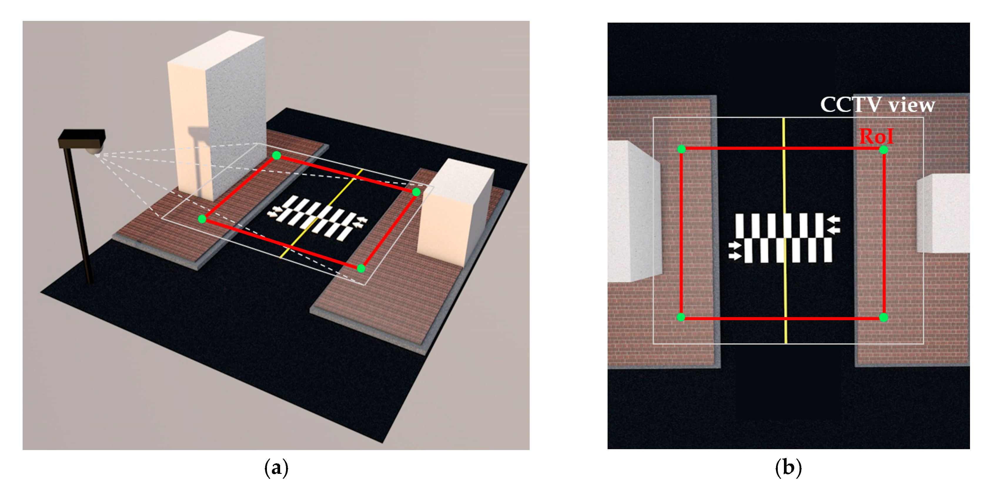
Next, with the recognized ground tip points, we transformed them into an overhead perspective using the “transformation matrix” within the OpenCV library. The transformation matrix can be derived from four pairs of corresponding “anchor points” in real image (oblique view) and virtual space (overhead view). Figure 5 represents the anchor points as green points from the two perspectives. In our experiment, we used the four corners of the rectangular crosswalk area as anchor points. We measured the real length and width of the crosswalk area on-site, then reconstructed it in virtual space from an overhead perspective with proportional dimensions, oriented orthogonally to the x–y plane. We then identified the vertex coordinates of the rectangular crosswalk area in the camera image and the corresponding vertices in our virtual space, and used these to initialize the OpenCV function to apply to all detected contact points. A similar procedure for perspective transformation is also described in detail in [24].
2.4. Object Behavioral Feature Extraction
In this section, we describe how to extract the objects’ behavioral features from the recognized overhead contact point. Vehicles and pedestrians exist as contact points in each individual frame. To estimate velocity and acceleration, we must identify each object in successive frames and link them into trajectories. The field of computer vision has developed many successful strategies for object tracking [25,26,27]. In this study, we applied a simple and low-computational tracking and indexing algorithm, since most unsignalized crosswalks are on narrow roads with light pedestrian traffic [25,27]. The algorithm identifies each individual object in consecutive frames by using the threshold and minimum distances of objects. For example, assume that there are three detected object (pedestrian) positions in the first frame named A, B, and C, and in the second frame named D, E, and F, respectively (see Figure 6).
There are multiple object positions defined as x–y coordinates (contact points) in each frame, and each object has a unique identifier (ID) ordered by detection accuracy. In Figure 6, A and B in the first frame move to E and F in the second frame, respectively. C moves to somewhere out-of-frame, while D emerges in the second frame.
To ascertain the trajectories of each object, we set frame-to-frame distance thresholds for vehicles and pedestrians, and then compare all distances between positions from the first to the second frame, as seen in Table 1. In this example, if we set the pedestrian threshold at 3.5, C is too far from either position in the second, but within range of the edge of the frame. When A is compared with D, E, and F, it is closest to E; likewise, B is closest to F. We can infer that A moved to E, and B moved to F, while a pedestrian at C left the frame, and D entered the frame. We apply this algorithm to each pair of consecutive frames in the dataset to rebuild the full trajectory of each object.
With the trajectories of these objects, we can extract the object’s behavioral features which affect the potential risk. At each frame, we extracted five behavioral features for each object: Vehicle velocity (VV), vehicle acceleration (VA), pedestrian velocity (PV), distance between vehicle and pedestrian (DVP), and distance between vehicle and crosswalk (DVC). The extracting methods are described below in detail.
Vehicle and pedestrian velocity (VV and PV): In general, object velocity is a basic measurement that can signal the likelihood of potentially dangerous situations. The speed limit in our testbed, spots A and B, is 30 km/h, so if there are many vehicles detected driving over this limit at any point, this contributes to the risk of that location. Pedestrian velocity alone is not an obvious factor for risk, but when analyzed together with other features, we may find important correlations and interactions between the object velocities and the likelihood for pedestrian risk.
Velocity of objects is calculated by dividing an object’s distance moving between frames by the time interval between the frames. In our experiment, videos were recorded at 15 and 11 fps in spots A and B, respectively, and sampled at every fifth frame. Therefore, the time interval F between two consecutive frames was 1/3 s in spot A, and 5/11 s, in spot B. Meanwhile, pixel distance in our transformed overhead points was converted into real-world distance in meters. We infer pixel-per-meter constant (P) using the actual length of the crosswalks as our reference point. In our experiment, the actual length of both crosswalks in spots A and B were 15 m, and the pixel lengths of these crosswalks were 960 pixels. Thus, object velocity was calculated as:
The unit is finally converted into km/h.
Vehicle acceleration (VA): Vehicle acceleration is also an important factor to determine the potential risk for pedestrian injury. In general, while vehicles pass over a crosswalk with a pedestrian nearby, they reduce speed (resulting in negative acceleration values). If many vehicles maintain speed (zero value) or accelerate (positive values) while nearby the crosswalk or pedestrian, it can be considered as a risky situation for pedestrians.
Vehicle acceleration is the difference between vehicle velocities in the current frame () and in the next frame ():
The unit is finally converted into km/h2.
Distance between vehicle and pedestrian (DVP): This feature refers to the physical distance between each vehicle and pedestrian. In general, if this distance is short, the driver should slow down with additional caution. However, if the vehicle has already passed the pedestrian, accelerating presents less risk than when the pedestrian ahead of the car. Therefore, we measure DVP to distinguish between these types of situations. If a pedestrian is ahead of the vehicle, the distance has a positive sign, if not, it has a negative sign:
Distance between vehicle and crosswalk (DVC): This feature is also extracted by calculating the distance between vehicle and crosswalk. We measure this distance from the crosswalk line closest to the vehicle; when vehicle is on the crosswalk, the distance is 0:
As a result of feature extraction, we can obtain a structured dataset suitable for various data mining techniques, as seen in Table 2.
2.5. Data Mining Techniques for PPRE Analysis
In this section, we describe two data mining techniques used to elicit useful information for an in-depth understanding of potential pedestrian risky events: K-means clustering and decision tree methods.
K-means clustering: Clustering techniques consist of unsupervised and semi-supervised learning methods and are mainly used to handle the associations of some characteristic features [28]. In this study, we considered each frame with its extracted features as a record, and used k-means clustering to classify them into categories which could indicate degrees of risk. The basic idea of k-means clustering is to classify the dataset D into K different clusters, with the classified clusters consisting of the elements (records or frames) denoted as . The set of elements between classified clusters is disjointed, and the number of elements in each cluster is denoted by . The k-means algorithm consists of two steps [29]. First, the initial centroids for each cluster are chosen randomly, then each point in the dataset is assigned to its nearest centroid by Euclidean distance [30]. After the first assignment, each cluster’s centroid is recalculated for its assigned points. Then, we alternate between reassigning points to the cluster of its closest centroid, and recalculating those centroids. This process continues until the clusters no longer differ between two consecutive iterations [31].
In order to evaluate the results of k-means clustering, we used the elbow method with the sum of squared errors (SSE). SSE is the sum of squared differences between each observation and mean of its group. It can be used as a measure of variation within a cluster, and the SSE is calculated as follows:
where is the number of observations , which is a value of the i-th observation, and is the mean of all the observations.
We ran k-means clustering on the dataset for a certain range of values of K, and calculate the SSE for each result. If the line chart of SSE plotted against K resembles an arm, then the “elbow” on the arm represents a point of diminishing returns when increasing K. Therefore, with the elbow method, we selected an optimal number of K clusters without overfitting our dataset. Then, we validated the accuracy of our clustering by using the decision tree method.
Decision tree: Decision trees are widely used to model classification processes [32,33]. It is one of many supervised learning algorithms, and can effectively divide a dataset into smaller subsets [34]. It takes a set of classified data as input, and arranges the outputs into a tree structure composed of nodes and branches.
There are three types of nodes: (1) root node, (2) internal node, and (3) leaf node. Root nodes represent a choice that will result in the subdivision of all records into two or more mutually exclusive subsets. Internal nodes represent one of the possible choices available at that point in the tree structure. Lastly, the leaf node, located at the end of the tree structure, represents the final result of a series of decisions or events [35,36]. Since a decision tree model forms a hierarchical structure, each path from the root node to leaf node via internal nodes represents a classification decision rule. These pathways can be also described as “if-then” rules [36]. For example, “if condition 1 and condition 2 and … condition k occur, then outcome j occurs.”
In order to construct a decision tree model, it is important to split the data into subtrees by applying criteria such as information gain and gain ratio. In our experiment, we applied the popular C4.5 decision tree algorithm, an extended algorithm of ID3 that uses information gain as its attribute selection measure. Information gain is based on the concept of entropy of information, referring to the reduction of the weight of desired information, which then determines the importance of variables [35]. C4.5 decision tree algorithm selects the attribute of the highest information gain (minimum entropy) as the test attribute of the current node. Information gain is calculated as follows:
where is a given data partition, and is the attribute (the extracted five features in our experiment). is split into partitions (subsets) as . Entropy is calculated as follows:
where is derived from , and has non-zero probability that an arbitrary tuple in belongs to class (cluster, in our experiment) . The attribute with the highest information gain is selected. In the decision tree, entropy is a numerical measure of impurity, and is the expected value for information. The decision tree is constructed to minimize impurity.
Note that in order to minimize entropy, the decision tree is constructed to maximize information gain. However, information gain is biased toward attributes with many outcomes, referred to as multivalued attributes. To address this challenge, we used C4.5 with “gain ratio”. Unlike with information gain, the split information value represents the potential information generated by splitting the training dataset into partitions, corresponding to outcomes on attribute . Gain ratio are used for split criteria and calculated as follows [37,38]:
The attribute with the highest gain ratio will be chosen for splitting attributes.
In our experiment, there are two reasons for using the decision tree algorithm. First, we can validate the result of the k-means clustering algorithm. Unlike k-means clustering, the performance of the decision tree can be validated through its accuracy, precision, recall, and F1 score. Precision is the ratio of positive classification to the classified results, and recall is the ratio of data successfully classified in the input data [37,39].
where TP is true positive, FP is false positive, and FN is false negative.
Second, we can analyze the decision tree results in-depth, by treating them as a set of “if-then” rules applying to every vehicle–pedestrian interaction at that location. At the end of Section 3, we will discuss the results of the decision tree and confirm the feasibility and applicability of the proposed PPRE analysis system by analyzing these rules.
3. Experiments and Results
3.1. Experimental Design
In this section, we describe the experimental design for k-means clustering and decision trees as core methodologies for the proposed PPRE analysis system. First, we briefly explain the results of data preprocessing and statistical methodologies. The total number of records (frames) is 4035 frames (spot A: 2635 frames and spot B: 1400 frames). Through preprocessing, we removed outlier frames based on extreme feature values, yielding 2291 and 987 frames, respectively. We then conducted [0, 1] normalization on the features as follows:
Prior to the main analyses, we conducted statistical analyses such as histogram and correlation analysis. Figure 7a–f illustrated histograms of all features and each feature, respectively. VV and PV features are skewed low since almost all cars and pedestrians stopped or moved slowly in these areas. Averages of VV and PV are at about 24.37 and 2.5 km/h, respectively. When considering speed limits are 30 km/h in these spots, and the average person’s speed is approximately 4 km/h, these are reasonable values. DVP (distance from vehicle to pedestrian) shows two local maxima: One for pedestrians ahead of the car, and one for behind.
Next, we can study the relationships between each feature by performing correlation analysis. Figure 8a,b represents correlation matrices in spots A and B. In spot A, we can observe negative correlation between VV and DVP. This indicates that vehicles tended to move quickly near pedestrians, indicating a dangerous situation for the pedestrian. In spot B, there is negative correlation between PV and DVP, which could be interpreted in two ways: Pedestrians moved quickly to avoid a near-miss by an approaching car, or pedestrians slowed down or stopped altogether to wait for the car to pass nearby. Since we extracted only video clips containing scenes where at least one pedestrian and one car were in the camera view at the same time, DVP and DVC have positive correlation.
For our experiment, we conducted both quantitative and qualitative analyses. In the quantitative analysis, we performed k-means clustering to obtain the optimal number of clusters (K). Each clustering experiment was evaluated by the SSE depending on K between 2 to 10, and through the elbow method, we chose the optimal K. Then, we used the decision tree method to validate the classified dataset with a chosen K. The proportion of training and test data were at about 70% (2287 frames) and 30% (991 frames), respectively. In the qualitative analysis, we analyzed each feature and its relationship with multiple other features by clustering them. Then, we analyzed the rules derived from the decision tree and their implications for the behavior and safety at the two sites.
3.2. Quantitative Analysis
In order to obtain the optimal number of clusters, K, we looked at the sum of squared errors between the observations and centroids in each cluster by adjusting K from 2 to 10 (see Figure 9). SSE decreases with each additional cluster, but when considering computational overhead, the curve flattens at K = 6. Thus, we set the optimal K at 6, which means that the five behavioral features could be sufficiently classified into six categories.
As a result of this clustering method, we obtained the labels (i.e., classes or categories). Since this is an unsupervised learning model, and since the elbow method is partly subjective, we need to ensure that the derived labels are well classified.
Thus, with the chosen K, we performed the decision tree classifier as a supervised model, and used the following parameter options for learning process: a gain ratio for split criterion, max tree depth of 5, and binary tree structure. As a result, Table 3 shows the confusion matrix, with the accuracy remaining at 92.43%, and the average precision, recall, and F1-score all staying at 0.92.
Thus, with the k-means clustering and decision tree methods, we determined an optimal number of clusters (6), and evaluated the performance of the derived clusters.
3.3. Qualitative Analysis
We scrutinized the distributions and relationships between each two features, and clarified the meaning of each cluster by matching each cluster’s classification rules and the degree of PPRE. This section consists of three parts: (1) Boxplot analysis for single feature by cluster, (2) scatter analysis for two features, and (3) rule analysis by decision tree.
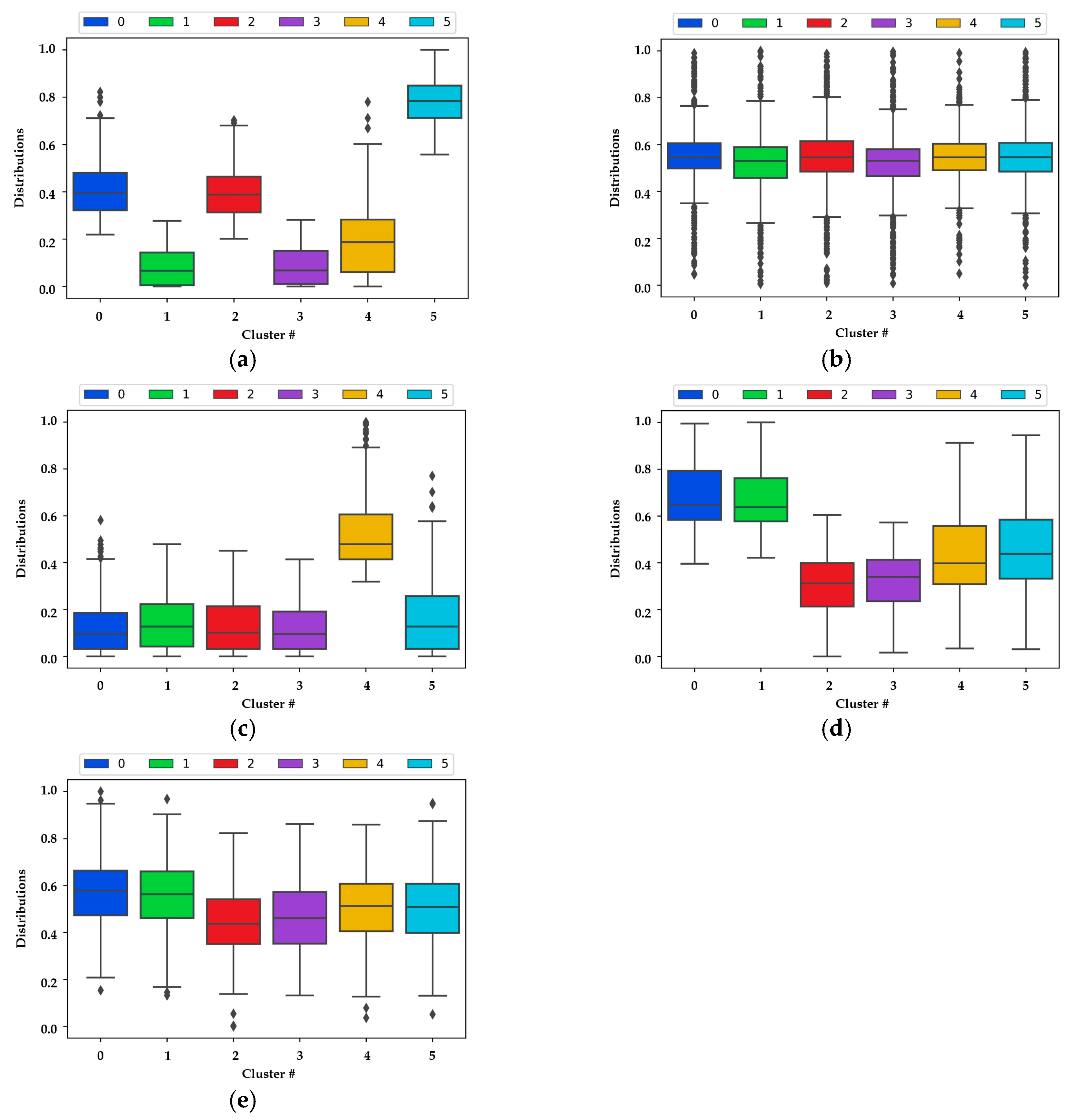
First, we viewed the boxplot grouped by cluster, as illustrated in Figure 10a–e, as distributions of VV, VA, PV, DVP, and DVC features, respectively. In Figure 10a, cluster #5 is skewed higher than others, and this would distinguish it from the others overall. In Figure 10b,e, most frames are evenly allocated to each cluster, and a clear line does not seem to exist for their classification. In Figure 10c, we can see that in cluster #4, most frames are associated with high walking speed. In Figure 10d, cluster #0 and #1 are skewed higher than others, and have similar means and deviations. Comprehensively, cluster #5 has high VV and low PV, and cluster #4 has low VV and high PV. Cluster #0 and #1 have high DVP, but cluster #0 has moderate VV, and cluster #1 has low VV. As above results reveal, partial clusters have distinguishable features. However, boxplot analysis only illustrates a single feature, limiting its use in clearly defining the degrees of PPRE.
Second, we performed the correlation analysis between two features by using scatter matrices as illustrated in Figure 11. This figure describes the comprehensive results for labeled frames by hue and correlations between each feature.
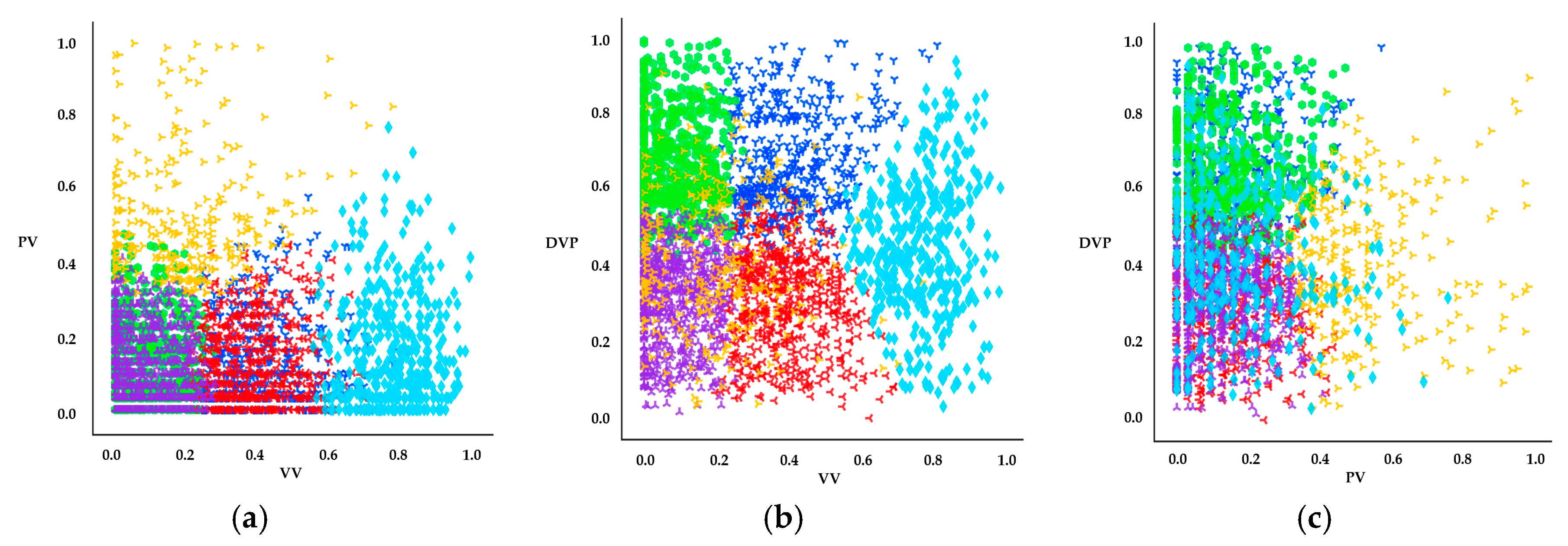
We studied three cases which are well-marked in detail (see Figure 12a–c). Figure 12a represents the distributions between VV and PV features by cluster. Cluster #5 features high-speed cars and slow pedestrians. This could be interpreted as moments when pedestrians walk slowly or stop to wait for fast-moving cars to pass by. Cluster #4 could be similarly interpreted as moments when cars stop or drive slowly to wait for pedestrians to quickly cross the street.
Figure 12b illustrates the scatterplot between VV and DVP features. Remarkably, most clusters appear well-defined except for cluster #4. For example, cluster #3 has low VV and low DVP, for cars slowing or stopped while near pedestrians. Cluster #2 has higher VV than those of cluster #3 and low DVP, representing cars that move quickly while near pedestrians. Cluster #5 seems to capture vehicles traveling at high speeds regardless of their distance from pedestrians.
Finally, Figure 12c shows the relationships between PV and DVP. In this figure, cluster #1 has low PV and high DVP, capturing pedestrians walking slowly even when cars are far from them. In cluster #4, regardless of distance from cars, pedestrians run quickly to avoid approaching cars. Through these analyses, it is possible to know features’ distributions as allocated to each cluster, and to simply infer the type of PPRE that each cluster represents.
Finally, we visualized the decision tree and analyzed it in order to figure out how each cluster could be matched to degrees of PPRE. Note that the decision tree makes it possible to analyze the classified frames in detail in the form of “if-then” rules. Figure 13 shows the result of the full decision tree without pruning, representing all of the complicated rules in detail. However, for the purpose of this paper, we chose to simplify the tree and the derived rules by limiting their maximum depth to 5 levels. Figure 14 shows the simpler decision tree and Table 4 lists its derived rules.
In this figure, VV serves as the root node, reflecting its importance in classifying the given data. In addition, although we started with five features (VV, VA, PV, DVP, and DVC), only three features (VV, PV, and DVP) formed branches in this simplified decision tree. We focused on analyzing the rules for paths from root to leaf node, rather than what each node means within the context of the tree and subtrees. For example, if we follow the leftmost path from root node to the leaf node (VV is less than 21.6 km/h, DVP is less than 10.6 m, and PV is less than 3.1 km/h), then this rule matches cluster #3. Based on these “if-then” rules, we can interpret the patterns for each cluster. Table 4 shows all of the rules derived from this decision tree.
In cluster #1, cars are driving slowly, and pedestrians are at least 10 m away, while in cluster #3, cars are driving slowly but closer to the pedestrians, who are stopped or walking very slowly. Both of these represent safer situations than the other clusters.
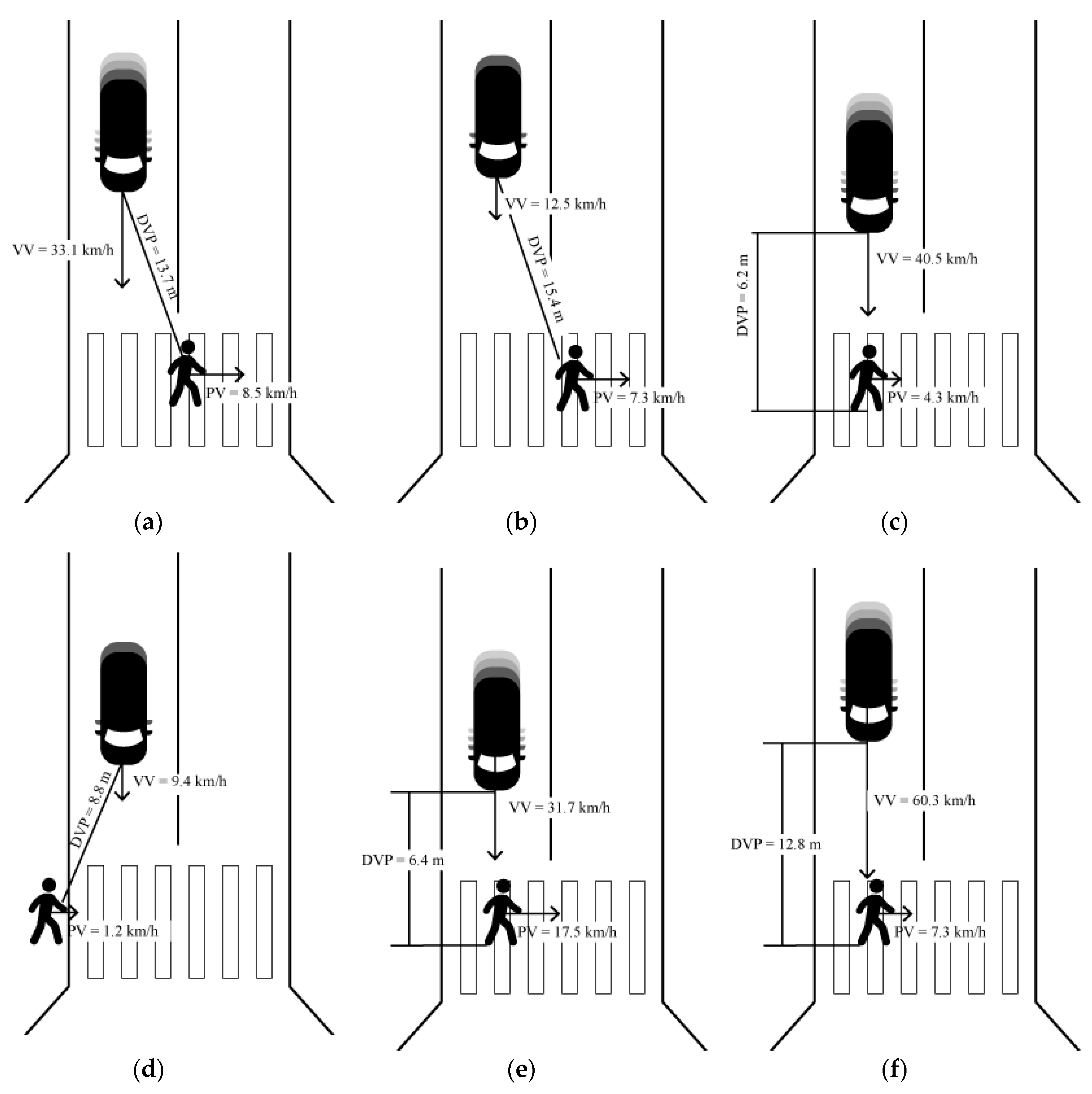
Cluster #0 encompasses two scenarios. First, vehicles are moving at moderate to high speeds, but pedestrians are sufficiently far away and walking somewhat quickly. Alternatively, cars are moving faster than the speed limit, but their distance from pedestrians is large. We interpret cluster #0 to represent potential (but not severe) risky situations. Similarly, cluster #2 shows vehicles driving at moderate speeds within 9 m of pedestrians, who are walking slowly. Cluster #4 includes three branches that parallel situations in clusters #1, #2, and #3, but with faster-moving pedestrians. Either pedestrians are moving quickly to avoid contact, or are entering the crosswalk at higher speeds, implying greater risk to the pedestrian.
We regarded cluster #5 as having the most dangerous situations, since vehicle velocities far exceeds the speed limit, at distances from pedestrians within ~15 m.
Comprehensively, we can match each rule (cluster) to a degree of PPRE. As a result, clusters #1 and #3 appear safe, while clusters #0, #2, and #4 are ambiguous but could represent risky situations for pedestrians. The risks in cluster #5 were much clearer.
3.4. Results in Summary
In this study, we aimed to detect traffic-related objects from video footage, extract their behavioral features, and classify the frames by using data mining techniques such as k-means clustering and decision trees. We applied our system using a large video dataset from Osan city, automatically extracted object trajectories and frame-level features, determined the optimal number of frame clusters using the elbow method with the sum of squared errors, and evaluated the result by using a decision tree. As a result, the accuracy of our model is at 92.43% when the optimal K is 6 clusters.
We then performed a boxplot analysis for single feature by cluster, scatter analysis for two features, and rule analysis derived from decision tree. While some clusters could be distinguished by boxplot, scatter plots provided clearer distinctions between the clusters. Rule analysis allowed us to interpret each cluster, and although three of the six clusters could be clearly identified as safe or dangerous situations, the remaining three clusters were more ambiguous in their potential risk to pedestrians. We also found that of our five initial features, only vehicle velocity, vehicle–pedestrian distance, and pedestrian velocity were needed to classify situations at a high level.
Figure 15 illustrates an example situation from each cluster, and the three behavioral features used to classify them.
3.5. Discussions
When preprocessing and extracting behavioral features, we handled video footage on an end-point server with direct access to the image feed from individual CCTV cameras (see Figure 3). Because we only worked with two cameras and processed one hour of footage from each day, our system could afford to run more slowly than real-time. However, it is possible to optimize the system to run at or faster than real-time, which will be necessary to expand the scale to larger urban areas with more cameras available, as well as longer daily study periods. The future goals of this study are to accumulate a large number of vehicle–pedestrian interaction events, in diverse environments and external conditions, and provide a dense dataset for other types of behavioral analysis.
Much research has been conducted on pedestrian safety evaluation at locations where they are vulnerable (e.g., mid-block crosswalks, intersections, school zones, etc.) by analyzing vehicle and pedestrian behaviors and their interactions based on vision sensors. Table 5 compares characteristics of previous systems with our approach. To assess potential risk, these systems extracted various standardized features from video footage, such as time-to-collision (TTC) or post-encroachment time (PET), but in practice, most relied on manual effort by a human observer. The closest approach to ours was [40], which similarly automated the entire process of object detection, tracking, and feature extraction, but focused on TTC at signalized intersections. By contrast, our process focused on unsignalized crosswalks, looked more generally at velocities and distances to assess risk, and introduced clustering as a new way to categorize types of risk event. Thus, we combine the advantages of automated feature extraction with machine learning to efficiently characterize potential risk events in these vulnerable locations.
In addition, by classifying potentially risky situations, we sought to create an objective metric that planners could use to compare different crosswalks, based on the relative frequency of these events at each location. Crosswalks dominated by “dangerous” clusters demand closer attention than those with mostly “safe” events. However, as our results show, there are still clusters of situations that, while distinct, are not easily classified as “safe” or “dangerous”.
Because vehicle–pedestrian interactions happen many times more often than actual accidents, this approach provides a richer, denser, more consistent perspective on the safety of these environments. We hypothesize that a much larger-scale PPRE dataset could actually be correlated with accident rates to clarify the relative risk of different types of event, or even predict accident rates based on observable driver/pedestrian behavior at the crosswalks. This could become part of a decision support system allowing transportation engineers or city planners to study existing areas, propose alternative road/intersection designs, and test the impact of these physical changes over relatively short timeframes. We plan to develop this decision support system in subsequent studies.
4. Conclusions
In this study, we demonstrated a system for classifying potential pedestrian risky events at unsignalized crosswalks, using data mining techniques on footage from existing traffic surveillance cameras. The core methodologies were to automatically recognize objects’ precise contact points (despite the oblique perspective of the camera footage), to extract their behavioral features through simple object tracking, and to classify the types of risk and analyze features in each class through data mining, visualization, and interpretation. We validated the feasibility of our proposed PPRE analysis model by implementing it with Tensorflow, OpenCV libraries, and k-means clustering and decision tree algorithms in Python, and applying it to actual video data from unsignalized crosswalks in Osan city, South Korea.
Our results show the potential value and limits of information derived from such video data, in identifying situations and places where potential pedestrian risky events frequently occur. Such information can be harvested without great expense nor new infrastructure, specifically by repurposing security footage near roads to extract anonymized movement trajectories of vehicles near pedestrians. Collecting this data at a large scale could help protect pedestrians by detecting potentially dangerous driving patterns in certain areas before accidents occur there. This research is the first step to develop safer mobility environments in smart cities. Further reinforcement of the proposed model is required and is a part of our ongoing work.
Author Contributions
B.N. and D.L. conceived and designed the experiments; B.N. and W.N. conducted experiments and implemented analysis system; and B.N., J.L., and D.L. wrote and revised the paper. All authors have read and agreed to the published version of the manuscript.
Funding
This work was financially supported by the National Research Foundation of Korea (NRF) grant funded by the Korea government (MSIT) (No. NRF-2018R1D1A1B07049129), and by Korea Ministry of Land, Infrastructure, and Transport (MOLIT) as “Innovative Talent Education Program for Smart City”.
Acknowledgments
We thank Osan smart city integrated operations center for providing CCTV videos, and Eunji Choi for help in drawing 3D space viewed figures. We also thank Hans Han for helping proofread this manuscript.
Conflicts of Interest
The authors declare no conflicts of interests.
References
- Ho, G.T.; Tsang, Y.P.; Wu, C.H.; Wong, W.H.; Choy, K.L. A computer vision-based roadside occupation surveillance system for intelligent transport in smart cities. Sensors 2019, 19, 1796. [Google Scholar] [CrossRef] [PubMed] [Green Version]
- Lytras, M.; Visvizi, A. Who uses smart city services and what to make of it: Toward interdisciplinary smart cities research. Sustainability 2018, 10, 1998. [Google Scholar] [CrossRef] [Green Version]
- Akhter, F.; Khadivizand, S.; Siddiquei, H.R.; Alahi, M.E.; Mukhopadhyay, S. IoT enabled intelligent sensor node for smart city: Pedestrian counting and ambient monitoring. Sensors 2019, 19, 3374. [Google Scholar] [CrossRef] [PubMed] [Green Version]
- Boufous, S.; Murray, C.J.L.; Vos, T.; Lozano, R.; Naghavi, M.; Global Burden of Disease Study 2010 Collaborators. 75 The rising global burden of road injuries. Injury Prev. 2016. [Google Scholar] [CrossRef] [Green Version]
- Gandhi, T.; Trivedi, M.M. Pedestrian protection systems: Issues, survey, and challenges. IEEE Trans. Intell. Transp. Syst. 2007, 8, 413–430. [Google Scholar] [CrossRef] [Green Version]
- Gitelman, V.; Balasha, D.; Carmel, R.; Hendel, L.; Pesahov, F. Characterization of pedestrian accidents and an examination of infrastructure measures to improve pedestrian safety in Israel. Accid. Anal. Prev. 2012, 44, 63–73. [Google Scholar] [CrossRef]
- Olszewski, P.; Szagała, P.; Wolański, M.; Zielińska, A. Pedestrian fatality risk in accidents at unsignalized zebra crosswalks in Poland. Accid. Anal. Prev. 2015, 84, 83–91. [Google Scholar] [CrossRef]
- Haleem, K.; Alluri, P.; Gan, A. Analyzing pedestrian crash injury severity at signalized and non-signalized locations. Accid. Anal. Prev. 2015, 81, 14–23. [Google Scholar] [CrossRef]
- Fu, T.; Hu, W.; Miranda-Moreno, L.; Saunier, N. Investigating secondary pedestrian-vehicle interactions at non-signalized intersections using vision-based trajectory data. Transp. Res. Part C Emerg. Technol. 2019, 105, 222–240. [Google Scholar] [CrossRef]
- Fu, T.; Miranda-Moreno, L.; Saunier, N. A novel framework to evaluate pedestrian safety at non-signalized locations. Accid. Anal. Prev. 2018, 111, 23–33. [Google Scholar] [CrossRef]
- Jiang, X.; Wang, W.; Bengler, K.; Guo, W. Analyses of pedestrian behavior on mid-block unsignalized crosswalk comparing Chinese and German cases. Adv. Mech. Eng. 2015, 7. [Google Scholar] [CrossRef]
- Murphy, B.; Levinson, D.M.; Owen, A. Evaluating the Safety in Numbers effect for pedestrians at urban intersections. Accid. Anal. Prev. 2017, 106, 181–190. [Google Scholar] [CrossRef]
- Kadali, B.R.; Vedagiri, P. Proactive pedestrian safety evaluation at unprotected mid-block crosswalk locations under mixed traffic conditions. Saf. Sci. 2016, 89, 94–105. [Google Scholar] [CrossRef]
- Onelcin, P.; Alver, Y. The crossing speed and safety margin of pedestrians at signalized intersections. Transp. Res. Procedia 2017, 22, 3–12. [Google Scholar] [CrossRef]
- Onelcin, P.; Alver, Y. Illegal crossing behavior of pedestrians at signalized intersections: Factors affecting the gap acceptance. Transp. Res. Part F Traffic Psychol. Behave. 2015, 31, 124–132. [Google Scholar] [CrossRef]
- Sochor, J.; Špaňhel, J.; Herout, A. Boxcars: Improving fine-grained recognition of vehicles using 3-d bounding boxes in traffic surveillance. IEEE Trans. Intell. Transp. Syst. 2018, 20, 97–108. [Google Scholar] [CrossRef] [Green Version]
- Hussein, M.; Sayed, T.; Reyad, P.; Kim, L. Automated pedestrian safety analysis at a signalized intersection in New York City: Automated data extraction for safety diagnosis and behavioral study. Transp. Res. Rec. 2015, 2519, 17–27. [Google Scholar] [CrossRef]
- Ren, S.; He, K.; Girshick, R.; Sun, J. Faster r-cnn: Towards real-time object detection with region proposal networks. Adv. Neural Inf. Process. Syst. 2015, 91–99. [Google Scholar] [CrossRef] [Green Version]
- Pham, M.T.; Lefèvre, S. Buried object detection from B-scan ground penetrating radar data using Faster-RCNN. In Proceedings of the IGARSS 2018—2018 IEEE International Geoscience and Remote Sensing Symposium, Valencia, Spain, 22–27 July 2018; pp. 6804–6807. [Google Scholar]
- Jiang, H.; Learned-Miller, E. Face detection with the faster R-CNN. In Proceedings of the 2017 12th IEEE International Conference on Automatic Face & Gesture Recognition (FG 2017), Washington, DC, USA, 30 May–3 June 2017; pp. 650–657. [Google Scholar]
- He, K.; Gkioxari, G.; Dollár, P.; Girshick, R. Mask r-cnn. In Proceedings of the IEEE International Conference on Computer Vision (ICCV), Venice, Italy, 22–29 October 2017; pp. 2961–2969. [Google Scholar]
- Github. Available online: https://github.com/tensorflow/models/tree/master/research/object_detection (accessed on 3 September 2019).
- COCO Dataset. Available online: http://cocodataset.org/#home (accessed on 3 September 2019).
- Noh, B.; No, W.; Lee, D. Vision-based Overhead Front Point Recognition of Vehicles for Traffic Safety Analysis. In Proceedings of the 2018 ACM International Joint Conference and 2018 International Symposium on Pervasive and Ubiquitous Computing and Wearable Computers, Singapore, 8–12 October 2018; pp. 1096–1102. [Google Scholar]
- Besse, P.C.; Guillouet, B.; Loubes, J.M.; Royer, F. Review and perspective for distance-based clustering of vehicle trajectories. IEEE Trans. Intell. Transp. Syst. 2016, 17, 3306–3317. [Google Scholar] [CrossRef] [Green Version]
- Yuan, G.; Sun, P.; Zhao, J.; Li, D.; Wang, C. A review of moving object trajectory clustering algorithms. Artif. Intell. Rev. 2017, 47, 123–144. [Google Scholar] [CrossRef]
- Zuo, S.; Jin, L.; Chung, Y.; Park, D. An index algorithm for tracking pigs in pigsty. In Proceedings of the International Conference on Information Technology and Management Science, Hong Kong, China, 1–2 May 2014; pp. 1–2. [Google Scholar]
- Takyi, K.; Bagga, A.; Goopta, P. Clustering Techniques for Traffic Classification: A Comprehensive Review. In Proceedings of the 2018 7th International Conference on Reliability, Infocom Technologies and Optimization (Trends and Future Directions) (ICRITO), Noida, India, 14–17 October 2018; pp. 224–230. [Google Scholar]
- Mahmud, S.; Rahman, M.; Akhtar, N. Improvement of K-means clustering algorithm with better initial centroids based on weighted average. In Proceedings of the 2012 7th International Conference on Electrical and Computer Engineering, Dhaka, Bangladesh, 20–22 December 2012. [Google Scholar]
- Han, J.; Pei, J.; Kamber, M. Data Mining: Concepts and Techniques; Elsevier: Amsterdam, The Netherlands, 2011. [Google Scholar]
- Starczewski, A. A new validity index for crisp clusters. Pattern Anal. Appl. 2017, 20, 687–700. [Google Scholar] [CrossRef] [Green Version]
- Pandya, R.; Pandya, J. C5. 0 algorithm to improved decision tree with feature selection and reduced error pruning. Int. J. Comput. Appl. 2015, 117, 18–21. [Google Scholar] [CrossRef]
- Hssina, B.; Merbouha, A.; Ezzikouri, H.; Erritali, M. A comparative study of decision tree ID3 and C4. 5. Int. J. Adv. Comput. Sci. Appl. 2014, 4, 13–19. [Google Scholar]
- Dai, Q.Y.; Zhang, C.P.; Wu, H. Research of decision tree classification algorithm in data mining. Int. J. Database Theory Appl. 2016, 9, 1–8. [Google Scholar] [CrossRef]
- Song, Y.Y.; Ying, L.U. Decision tree methods: Applications for classification and prediction. Shanghai Arch. Psychiatry 2015, 27, 130. [Google Scholar]
- Han, J.; Kamber, M.; Pei, J. Data Mining Concepts and Techniques, 3rd ed.; Morgan Kaufmann: Morgan Kaufmann, MA, USA, 2011; pp. 83–124. [Google Scholar]
- Gupta, B.; Rawat, A.; Jain, A.; Arora, A.; Dhami, N. Analysis of various decision tree algorithms for classification in data mining. Int. J. Comput. Appl. 2017, 163, 15–19. [Google Scholar] [CrossRef]
- Chen, C.H. Handbook of Pattern Recognition and Computer Vision; World Scientific: London, UK, 2015. [Google Scholar]
- Powers, D.M. Evaluation: From precision, recall and F-measure to ROC, informedness, markedness and correlation. J. Mach. Learn. Technol. 2011. Available online: https://www.researchgate.net/publication/276412348_Evaluation_From_precision_recall_and_F-measure_to_ROC_informedness_markedness_correlation (accessed on 3 September 2019).
- Islam, M.; Rahman, M.; Chowdhury, M.; Comert, G.; Deepak Sood, E.; Apon, A. Vision-based Pedestrian Alert Safety System (PASS) for Signalized Intersections. arXiv 2019, arXiv:1907.05284. [Google Scholar]
- Wu, J.; Radwan, E.; Abou-Senna, H. Assessment of pedestrian-vehicle conflicts with different potential risk factors at midblock crossings based on driving simulator experiment. Adv. Transp. Stud. 2018, 44, 33–46. [Google Scholar]
- Fu, T.; Miranda-Moreno, L.; Saunier, N. Pedestrian crosswalk safety at nonsignalized crossings during nighttime: Use of thermal video data and surrogate safety measures. Transp. Res. Rec. 2016, 2586, 90–99. [Google Scholar] [CrossRef]
- Xie, K.; Li, C.; Ozbay, K.; Dobler, G.; Yang, H.; Chiang, A.T.; Ghandehari, M. Development of a comprehensive framework for video-based safety assessment. In Proceedings of the 2016 IEEE 19th International Conference on Intelligent Transportation Systems (ITSC), Rio de Janeiro, Brazil, 1–4 November 2016; pp. 2638–2643. [Google Scholar]
- Passant, R.; Sayed, T.; Zaki, N.H.; Ibrahim, S.E. School zone safety diagnosis using automated conflicts analysis technique. Can. J. Civ. Eng. 2017, 44, 802–812. [Google Scholar]
Figure 1.
Closed-circuit television (CCTV) views in (a) spot A; and (b) spot B.

Figure 2.
Diagrams of objects’ trajectories in (a) spot A; and (b) spot B in overhead view.

Figure 3.
Overall architecture of the proposed analysis system.

Figure 4.
Ground point of pedestrian for recognizing its overhead view point.

Figure 5.
Example of perspective transform from (a) oblique view; into (b) overhead view.

Figure 6.
Example of object positions in two consecutive frames.

Figure 7.
Histograms of (a) all features; (b) VV; (c) VA; (d) PV; (e) DVP; and (f) DVC.

Figure 8.
Correlation matrices in (a) spot A; and (b) spot B.

Figure 9.
Sum of squared errors with elbow method for finding optimal K.

Figure 10.
Boxplots of (a) VV; (b) VA; (c) PV; (d) DVP; and (e) DVC by clusters.

Figure 11.
Result of correlation analysis using scatter matrices by clusters.

Figure 12.
Cluster distributions of (a) VV–PV; (b) VV–DVP; and (c) PV–DVP.

Figure 13.
Result of decision tree (no pruning).

Figure 14.
Result of decision tree with pruning.

Figure 15.
Examples of objects’ states based on rules in (a) cluster #0; (b) cluster #1; (c) cluster #2; (d) cluster #3; (e) cluster #4; and (f) cluster #5.
Figure 15.
Examples of objects’ states based on rules in (a) cluster #0; (b) cluster #1; (c) cluster #2; (d) cluster #3; (e) cluster #4; and (f) cluster #5.


Table 1.
Result of tracking and indexing algorithm using threshold and minimum distance.
| Object ID in First Frame | Object ID in Second Frame | Distance (m) | Result |
|---|---|---|---|
| A | D | 4.518 | Over threshold |
| A | E | 1.651 | Min. dist. |
| A | F | 2.310 | |
| B | D | 3.286 | |
| B | E | 2.587 | |
| B | F | 1.149 | Min. dist. |
| C | D | 7.241 | Over threshold |
| C | E | 5.612 | Over threshold |
| C | F | 3.771 | Over threshold |
Table 2.
Example of the structured dataset for analysis.
| Spot # | Event # | Frame # | VV (km/h) | VA (km/h2) | PV (km/h) | DVP (m) | DVC (m) |
|---|---|---|---|---|---|---|---|
| 1 | 1 | 1 | 19.3 | 5.0 | 3.2 | 12.1 | 8.3 |
| 1 | 1 | 2 | 16.6 | −2.1 | 2.9 | −11.4 | 6.2 |
| … | |||||||
| 1 | 529 | 8 | 32.1 | 8.4 | 4.1 | 8.0 | 0 |
| 2 | 1 | 1 | 11.8 | 1.2 | 3.3 | 17.2 | 18.3 |
| 2 | 1 | 2 | 9.5 | 0.3 | 2.7 | 7.8 | 4.3 |
| … | |||||||
| 2 | 333 | 12 | 22.3 | 1.6 | 7.2 | 3.3 | 2.3 |
…: It means that the records are still listed
Table 3.
Confusion matrix.
| Expected Class | Actual Class | |||||
|---|---|---|---|---|---|---|
| 0 | 1 | 2 | 3 | 4 | 5 | |
| 0 | 137 | 1 | 4 | 0 | 1 | 2 |
| 1 | 1 | 212 | 0 | 8 | 1 | 0 |
| 2 | 7 | 0 | 156 | 5 | 2 | 3 |
| 3 | 0 | 7 | 6 | 240 | 1 | 0 |
| 4 | 0 | 3 | 4 | 6 | 75 | 0 |
| 5 | 4 | 0 | 7 | 0 | 2 | 96 |
Table 4.
Rules derived from decision tree.
| Cluster # | Rules |
|---|---|
| 0 | VV > 21.6 km/h and DVP > 9.2 m and PV <= 10.2 km/h or 54.5 km/h < VV <= 65.4 km/h and DVP > 15.6 m |
| 1 | VV <= 21.6 km/h and DVP > 10.6 m and PV <= 7.8 km/h |
| 2 | 21.6 km/h < VV <= 54.5 km/h and DVP <= 9.2 m and PV <= 6.6 km/h |
| 3 | VV <= 21.6 km/h and DVP <= 10.6 m and PV <= 3.1 km/h |
| 4 | VV <= 21.6 km/h and DVP <= 10.6 m and PV > 3.1 km/h or VV <= 21.6 km/h and 10.6 m < DVP <= 12.3 m and PV > 7.8 km/h or 21.6 km/h < VV <= 54.5 km/h and DVP <= 9.2 m and PV > 6.6 km/h |
| 5 | VV >= 54.5 km/h and DVP <= 15.6 m and PV <= 11.7 km/h |
Note: Vehicle velocity = VV, vehicle acceleration = VA, pedestrian velocity = PV, vehicle–pedestrian distance = DVP, vehicle–crosswalk distance = DVC.
Table 5.
Comparison table for characteristics of previous systems with our approach.
| Data Source | Target Spot | Object Detection | Object Identification and Tracking | Feature Extraction | Used Features | |
|---|---|---|---|---|---|---|
| Ref [13] | CCTV camera | Unsignalized mid-block crosswalk | x | n/a | x | Pedestrian safety margin |
| Ref [14] | CCTV camera | Signalized intersections | x | n/a | x | Crossing speed, pedestrian delay, etc. |
| Ref [15] | CCTV camera | Signalized intersections | x | n/a | x | Gender, vehicle type, crossing speed, etc. |
| Ref [17] | CCTV camera | Signalized intersections | x | n/a | x | TTC, pedestrian gait, etc. |
| Ref [40] | CCTV camera | Signalized intersection | + | + | + | TTC, etc. |
| Ref [41] | Driving simulator data | Mid-block crosswalk | x | n/a | n/a | Maximum deceleration, TTC, PET, etc. |
| Ref [42] | Thermal video camera | Unsignalized crosswalk | x | n/a | x | Object speed, PET, yielding compliances, conflict rates, etc. |
| Ref [43] | CCTV camera | Intersections | n/a | + | + | Object trajectory, TTC, etc. |
| Ref [44] | CCTV camera | School zone roads | n/a | + | + | Object trajectory, VV |
| Proposed System | CCTV camera | Unsignalized crosswalk | + | + | + | VV, VA, PV, DVP and DVC |
Note: x: Manual extraction, +: Automated extraction, n/a: Not applicable, TTC: Time to collision, PET: Post-encroachment time.
© 2020 by the authors. Licensee MDPI, Basel, Switzerland. This article is an open access article distributed under the terms and conditions of the Creative Commons Attribution (CC BY) license (http://creativecommons.org/licenses/by/4.0/).
Share and Cite
MDPI and ACS Style
Noh, B.; No, W.; Lee, J.; Lee, D. Vision-Based Potential Pedestrian Risk Analysis on Unsignalized Crosswalk Using Data Mining Techniques. Appl. Sci. 2020, 10, 1057. https://doi.org/10.3390/app10031057
AMA Style
Noh B, No W, Lee J, Lee D. Vision-Based Potential Pedestrian Risk Analysis on Unsignalized Crosswalk Using Data Mining Techniques. Applied Sciences. 2020; 10(3):1057. https://doi.org/10.3390/app10031057
Chicago/Turabian StyleNoh, Byeongjoon, Wonjun No, Jaehong Lee, and David Lee. 2020. "Vision-Based Potential Pedestrian Risk Analysis on Unsignalized Crosswalk Using Data Mining Techniques" Applied Sciences 10, no. 3: 1057. https://doi.org/10.3390/app10031057
Note that from the first issue of 2016, this journal uses article numbers instead of page numbers. See further details here.