A New Face Recognition Method for Intelligent Security


1
School of Information Science and Engineering, Hebei University of Science and Technology, Shijiazhuang 050018, China
2
School of Computer Science and Technology, Harbin Institute of Technology, Weihai 264209, China
3
School of Internet of Things and Software Technology, Wuxi Vocational College of Science and Technology, Wuxi 214028, China
*
Author to whom correspondence should be addressed.
Appl. Sci. 2020, 10(3), 852; https://doi.org/10.3390/app10030852
Submission received: 13 December 2019
/
Revised: 21 January 2020
/
Accepted: 21 January 2020
/
Published: 25 January 2020
(This article belongs to the Special Issue Cognitive Computing with Big Data System over Secure Internet of Things )
Abstract
:With the advent of the era of artificial intelligence and big data, intelligent security robots not only improve the efficiency of the traditional intelligent security industry but also propose higher requirements for intelligent security. Aiming to solve the problem of long recognition time and high equipment cost of intelligent security robots, we propose a new face recognition method for intelligent security in this paper. We use the Goldstein branching method for phase unwrapping, which can improve the three-dimensional (3D) face reconstruction effect. Subsequently, by using the three-dimensional face recognition method based on face radial curve elastic matching, different weights are assigned to different curve recognition similarity for weighted fusion as the total similarity for recognition. Experiments show that the method has a higher face recognition rate and is robust to attitude, illumination, and noise.
1. Introduction
In recent years, the domestic security industry market has developed rapidly. As intelligence becomes a major trend in the industry, intelligent security has gradually become the direction of the transformation and upgrading of security companies, and its proportion in the security industry will become increasingly larger. In 2019, the market size of China’s security industry was approximately 720 billion yuan. It is estimated that in 2020, intelligent security will create a market worth about 100 billion yuan, and intelligent security will be an important market in the security field. There is a wide range of applications of the Internet of Things in smart cities, civil security, and some focusing industries. Among these, biometric technology is one of the most important critical technologies. Face recognition technology research based on big data systems is of great significance. With the technology of big data and artificial intelligence developing rapidly, the big data environment not only provides a good basis for the in-depth development of face recognition systems but also realizes the sharing of feature databases in wider fields, which is helpful for achieving more abundant face feature databases. Therefore, face recognition and artificial intelligence are connected and interact safely and seamlessly with big data systems, which have become an important technical support in social security systems. Intelligent security robots with a face recognition function are being developed. This kind of intelligent security robot will be used in many public places to accurately scan human facial features, make judgments, and record personal data and behaviors in the cloud and feed back to the background. It is superior to the traditional surveillance camera and has great practical significance for the development of the security industry.
The current biometric technology [1] includes face recognition, fingerprint recognition, palm print recognition, iris recognition, etc. Face recognition is the focus of researchers in the fields of pattern recognition and computer vision. It has the characteristics of noncontact and non-aware biometrics, compared with other biometric technologies such as fingerprint recognition and iris recognition. Currently, most face recognition devices are mainly based on two-dimensional images [2], but these devices are susceptible to ambient light, background, and shooting angle. In order to overcome this shortcoming, the technologies of geometric information and relative position information, which belong to the technologies of three-dimensional (3D) face images, are widely used because of their relatively more stable nature. Mainstream 3D imaging technologies include stereo vision, structured light [3], time of flight (TOF), and binocular ranging. Therefore, face recognition based on 3D face data achieves a more accurate recognition result. In the context of big data, it can quickly and accurately automatically recognize human faces and apply face recognition technology to the perception system of security robots. We show a new method for face recognition for intelligence security in this paper.
To recognize 3D faces, we must first preprocess the reconstructed 3D face images. In the study of image processing, a method of describing a digital image as a vector in terms of a frequency histogram of graphs and mapping the image into a vector space through a graph transformation is presented [4]. There is also a method in which an image is encoded by a region adjacency graph (RAG), based on multicolored neighborhood (MCN) clustering algorithm [5]. Three-dimensional face recognition is divided into two parts: measurement and algorithm. As an important three-dimensional measurement method, grating projection measurement has the advantages of noncontact, low cost, and high precision and is widely used in industrial detection, reverse engineering, biomedicine, virtual reality, and other fields [6,7]. The projected grating phase method was first proposed by Tskeda [8] in 1982. Information on object height is obtained by demodulating the fringes that are previously modulated by the height on the surface of the object in this method. Common fringe projection measurement techniques include phase measuring profilometry (PMP) [9,10], Fourier transform profilometry (FTP) [11], and Moire profilometry (MP). Compared to Fourier transform profilometry and convolutional demodulation, phase measurement profilometry requires more fringe patterns and slightly longer acquisition time. However, PMP has advantages such as a simpler solving process, fewer computations, and a resistance to the background influence. The method directly finds the phase value in fringe patterns through mathematical calculations, and thus, we use PMP for the wrap phase in fringe patterns. The frequency of phase shifts determines speed and accuracy. Fewer phase shifts lead to a faster speed, but the accuracy is lower. Accordingly, more phase shifts help improve the accuracy it may reach, but the speed is slower. Considering the two factors of speed and accuracy, we use a four-step phase-shift method as the demodulation method of the fringe phase. We use an improved Goldstein branching method for a better quality of phase unwrapping patterns and achieve practical significance for the accuracy of 3D reconstruction in human faces.
There are also many researches on algorithms for 3D face recognition. The algorithm introduced by Vezzetti et al. [12] automatically recognizes six basic facial expressions (anger, disgust, fear, joy, sadness, and surprise) by dividing the face image into 79 regions and comparing the feature values obtained in each region with a threshold. In a study by Marcolin et al. [13], an algorithm is explored for face recognition by using geometric descriptors (such as mean, Gaussian, path, shape index, curvature, and coefficients of basic form) to extract 3D facial features and analyze them. In a study by Nonis and colleagues [14], a method which combines 2D and 3D facial features is used for facial expression analysis and recognition. In our daily life, the faces of criminal suspects are often blocked through camouflage, which causes certain difficulties in face recognition. Aiming at this problem, a detection method and repair strategy are proposed by providing a database and corresponding experiment [15]. Generally speaking, these 3D face recognition algorithms are divided into the following three main categories: spatial-based direct matching, overall feature matching, and local feature matching. Spatial-based direct matching directly performs similarity matching on surfaces without the extraction of features. Commonly used matching methods include iterative closest point (ICP) [16] and the Hausdorff distance method [17]. It has a good effect on the matching of rigid surfaces, but it is susceptible to expression changes since the human face is a nonrigid surface. Overall feature matching focuses on the overall features of 3D faces. Those methods include the apparent matching based on depth patterns and methods based on the extended Gaussian image (EGI). Local feature matching mainly extracts local features of human faces for matching. Beumier and Acheroy [18] extracted the center contour line through the most prominent point on the curves of human faces and two contour lines parallel to it and obtained similarities among three contour lines by comparing the curvature values on the selected contour lines. Further fusion among them then resulted in the similarity of the human face. However, this method only extracts three curves on human faces, which thus leads to a severe loss of curvature information and a relatively narrower representation. Samir et al. [19] extracted equal-depth contours on the depth pattern of human faces and calculated the geodesic distance between the equal-depth contours of the test face and the library set face on the Riemann space as their matching similarity. Berretti et al. [20] divided human faces into several equal geodetic areas according to the geodesic distance between points on the curved surface and nose-tip, and then used the positional relationship between the points on the corresponding geodetic areas for face recognition. Gökberket al. [21] extracted seven vertical contour curves on human faces and calculated the similarity between each corresponding curve. Then, the similarities were merged into a total similarity for face recognition. Therefore, we extract the side contour, horizontal contour, and other radial curves from the nose-tip point on the reconstructed 3D face and apply improved layered elastic matching and corresponding point-spacing matching. According to different influences of facial expressions in human faces, the method assigns different weights to different curve recognition similarities for a weighted fusion and thus obtains its total similarity for identification. This method achieves higher face reconstruction efficiency and recognition performance in the context of big data.
The rest of this paper is organized as follows. We introduce the 3D face recognition system in Section 2. Then we show the 3D face reconstruction method based on a grating projection method in Section 3. In Section 4 we propose the 3D face recognition method. In Section 5, experiments are carried out for verification, and the result of the method is presented.
2. System Introduction
In order to improve the efficiency of face reconstruction and face recognition of intelligent security robots, we propose a new method for face recognition of intelligent security in this paper. The general process of face recognition is obtaining face images, preprocessing, feature extraction, and target recognition. A 3D face image is obtained by reconstructing a 3D face image. During the 3D face reconstruction, a four-step phase-shifted fringe pattern is generated by a computer and transmitted to a projector. Then, it is projected onto the background surface and the surface of the object to be measured. The camera separately obtains the background fringe pattern and the deformed fringe pattern and transmits them to the computer. In the image preprocessing part, the computer acquires 3D face images by solving the wrapped phase value with the four-step phase-shift method, obtaining the unwrapped phase value with the optimized Goldstein branching method and calculating the height with the phase-to-height transformation formula. In the feature extraction part, the lateral contour lines, horizontal contour lines, and other radial curves emitted from the tip of the nose of the 3D human face are extracted, and then improved layered matching and point-distance matching are performed on different curves. In the target recognition part, we obtain the total similarity by assigning the two matching degrees with different weights and calculating the weighted fusion. Finally, recognition of the three-dimensional face is complete. The flow chart of face recognition is shown in Figure 1, the hardware system block diagram is shown in Figure 2, and the overall flow chart of software is shown in Figure 3.
3. Related Work
3.1. Optimized Goldstein Branching Method
The four-step phase-shift method is used as the demodulation method of the fringe phase in this paper, which modulates the grating fringe pattern projected onto the surface of the object, and then the phase unwrapping [22] is calculated. Common spatial phase algorithms for phase unwrapping include: row and column expansion, Goldstein branching [23], discrete cosine transform least squares (DCT), and Fourier transform least squares. Traditional Goldstein branching methods can eliminate the inconsistency of the phase unwrapping results due to the different integral paths and thus avoid the propagation of errors. However, the established branching tangent line is relatively long, and the phase may be incapable of unfolding due to the formation of a loop in areas with denser residual points. Therefore, to reduce the sum of the lengths of all branch tangent lines, we propose an improved Goldstein branching method, which combines the positive and negative residual points in the interferogram and uses the sum of the lengths of the tangent lines as the evaluation value to replace and re-establish the positive and negative residual points in the interferogram, which can effectively overcome the “island phenomenon” that is prone to occur in areas with denser residual points when the phase is unwrapped.
The Goldstein branching method connects and balances the residual points on the interferogram to find the branching tangent lines that need to be avoided when the phase is unwrapped. When the strategy of connecting residual points to branches differs, the branching tangent lines differ, and phase unwrapping will also have different results. To create a better effect on phase unwrapping, the length of branching tangent lines should be as short as possible, and the connection distance between the positive and negative residual points should be short as well. The probability of residual point occurrence is 1/100 to 1/1000 of the two interference images with a correlation value between 0.3 and 0.5. Assuming that the number of positive and negative residual points is N, then there are N! combinations. If the image is large, there will be many calculations for the optimal combination.
The steps of the optimized Goldstein branching method are as follows:
- (1)
- Identify the positive and negative residual points in the two-dimensional interferogram and mark the position of the residual points in the residual point map.
- (2)
- Take the positive residual point as the center and search within the radius of 5. If a negative residual point is found within the range, the pair of positive and negative residual points is defined as a “near-point pair”. If there is not any corresponding negative residual point within the range, this positive residual point is defined as a “far point”.
- (3)
- Center on the “far point” and gradually expand the search radius until all “far points” have found their negative residual points to become “far point pairs”.
- (4)
- Take the positive residual point of the “far point pair” as the center and carry out the search again. The search radius here is the length of the branching tangent line of the “far point pair”. Replace and re-establish all “near-point pairs” and “far point pairs” within the radius. The principle of replacement is based on whether the value of the function (fitness) is reduced, and the evaluation value (fitness) is shown in Equation (1).
- (5)
- If the evaluation value does not decrease after the replacement, replace the combination of the positive and negative residual points in the search radius and repeat step (4).
- (6)
- Perform steps (4) and (5) for all “far point pairs”.
As the fitness continues to decrease, the length of the branching tangent line also decreases. The above steps are repeated for all those virtually combined branch tangent lines until the evaluation value no longer decreases and tends to converge.
Through the aforementioned operation, the sum of the combined distances of the residual points tends to be the shortest, and the optimized branching tangent lines are obtained. If the replacements in step (3) are counted as an average of K times, all those calculations will require a total of K × N operations. Since K << N, the number of calculations will be greatly reduced compared to N!.
In MATLAB, we use the peaks function as the measured object, and the results obtained after phase unwrapping are shown in Table 1. To simulate some of the interference in the measurement environment, we added a uniform noise with a mean of 0 and a variance of 1.1258.
It can be seen that the Goldstein branching method partially failed to unwrap and forms unexpanded regions. The time takes longer by the least squares method. The improved branch cutting method makes the expansion effect better through a shorter branch tangent by connecting the positive and negative residual points. Thus, the optimized Goldstein branching method makes the results of 3D reconstruction more accurate and contributes to subsequent processing and use.
3.2. 3D Human Face Reconstruction
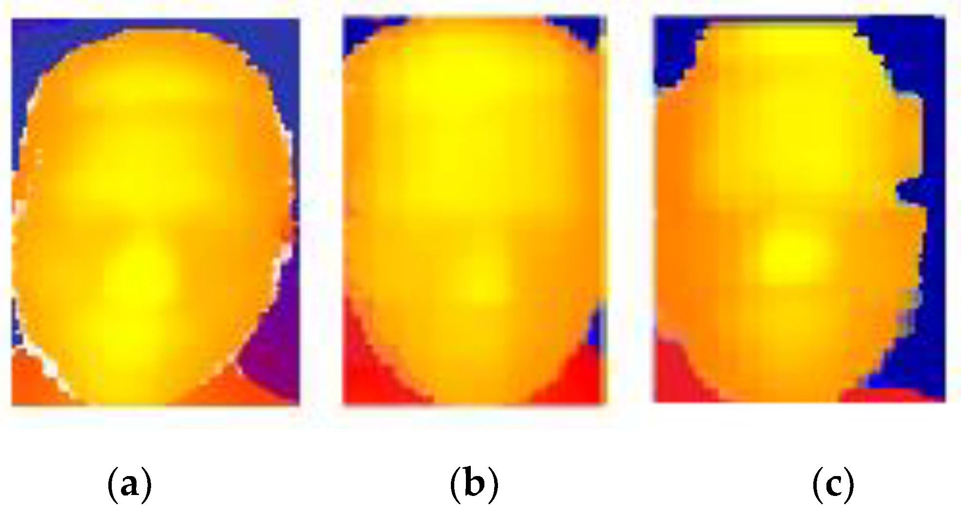
More accurate calculations are required for face recognition, and the quality of the image directly affects the accuracy of the recognition. Additionally, the number of projected fringes directly affects the accuracy of the wrapped phase values, which then affect the quality of the image. When the number of fringes is too large, the distance between them is very narrow. If the resolution of the projection device or the acquisition device cannot meet its requirements, the projected image or the fringe pattern obtained is severely deformed. Severely deformed fringe patterns result in serious errors in 3D face recognition. Therefore, to achieve more accurate 3D face feature positioning and recognition, we attempt to find the influence of the number of fringes on the reconstruction of 3D shapes using fringe patterns with different fringe numbers of 32, 64, and 128, respectively. The images collected are shown in Figure 4 and the reconstructed face image is shown in Figure 5.
It can be seen that when the number of fringes is 32, the projected image is not deformed, and a 3D face image with better quality is obtained; however, some details are missing in the image. When the number of fringes is 128, there are too many fringes in the projected image, which causes its deformation, and thus, the obtained 3D face image is severely deformed. When the number of fringes is 64, the projected image is not deformed, and the quality of the 3D face image is the best among the three images, with more details recovered in the human face. These details can make 3D face feature positioning and recognition more precise. Therefore, we chose the fringe pattern with 64 fringes.
The efficiency of 3D face reconstruction is significantly improved after the improvement of the branching method and the selection of the best number of fringes.
4. 3D Human Face Recognition Method
4.1. Extracting 3D Feature Curves
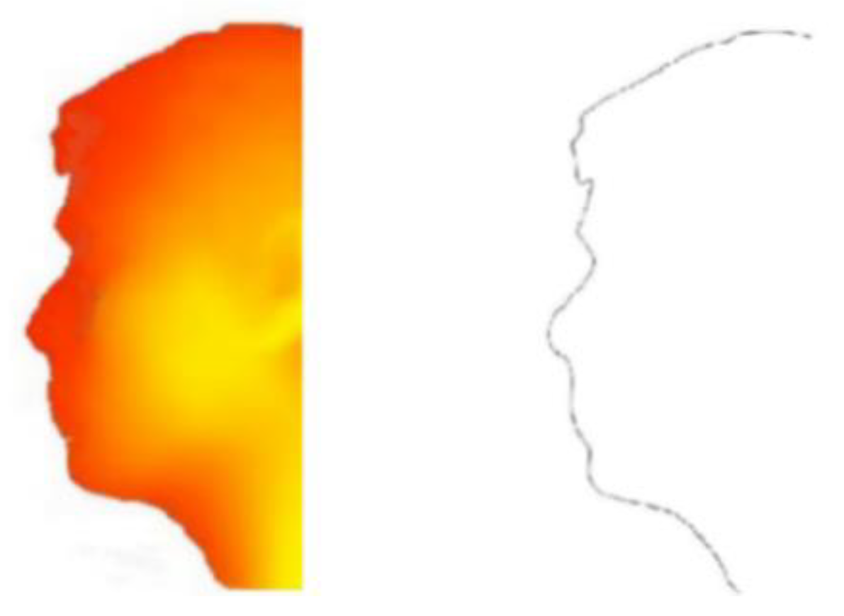
A 3D face image cannot contain all face information due to the difference in camera shooting angle and face posture change, which results in the lack of certain features in the face and affects the accuracy of recognition. The side contour of the face is the contour of the front end (highest height) when the face is facing sideways. It contains rich facial features and can represent the main features of the face compared to other characteristic curves [24]. There are certain differences between the side contours of different people, so using the face contour for face recognition achieves higher reliability and stability, as shown in Figure 6. The position of the side contour is determined according to the position of the two inner eye corners because the root of the nose is located in the center of the two eyes. The side contour is extracted according to the position of the tip of the nose and the root of the nose.
In addition to the side contour of the face, the horizontal contour across the nose-tip also has a good distinction and stability, as shown in Figure 7. The horizontal contour is extracted according to the tip of the nose and the position of the two inner corners of the eye. Then, we obtain the horizontal contour across the nose-tip. Using the 3D face positioning method based on the fringe and shape index, the positions of the nose-tip and the two inner eye corners in the image are found.
To retain most of the geometric information of the face and simplify the data volume of the three-dimensional face, we obtain a total of six reference curves with the nose-tip as the center of the sphere and across the mouth and eyes in its radial direction. We sample a point every 1.5 mm in those curves. For each point on the reference curve, the point on the radial curve that is closest to the distance dis in the direction of the reference curve and lesser than the threshold ζ = 0.3 is selected as the sampling point of the radial curve. In this way, a total of six characteristic curves with uniform sampling points are obtained, as shown in Figure 8.
4.2. Improved Layered Elastic Matching Method
The layered elastic matching algorithm based on the layered description of the two-dimensional deformation curve model captures the geometric shape information of the model, and thus is used for the shape analysis and similarity matching of the deformation model. Compared with the traditional deformation model analysis method, the layered deformation model has the advantage of calculating global geometric information in the elastic matching algorithm.
In the process of layered elastic matching, we introduce the concept of the shape tree. First, a shape tree is created for each curve of the library set face. Then, layered elastic matching is performed on the curve of the face in the test set. Finally, weighted fusion of all similarities yields layered matching similarity.
4.2.1. Establish a Shape Tree
We use open and ordered curves; A represents a curve consisting of a series of sampling points (a1, a2, …, an), and point ai on A is chosen as the midpoint, generally taking i = [(1 + n)/2]. L(ai|a1, an) is used to indicate the position of ai relative to ai and an. This is the Bookstein coordinate [25] of ai relative to a1 and an, that is, the coordinates obtained by mapping the first and last sampling points to a fixed position in a coordinate system. Due to the known position of the first and last sampling points, one Bookstein coordinate of an intermediate sampling point can well represent the relative positional relationship of the three points. First, mapping a1 to (−0.5, 0) and an to (0.5, 0), then the positions L(ai|a1, an) = (a(1), a(2)) and (a(1), a(2)) of ai relative to a1 and an are obtained by Equation (2):
where and (a(1), a(2)) are two-dimensional coordinates of ak (k = 1, 2, …, n).
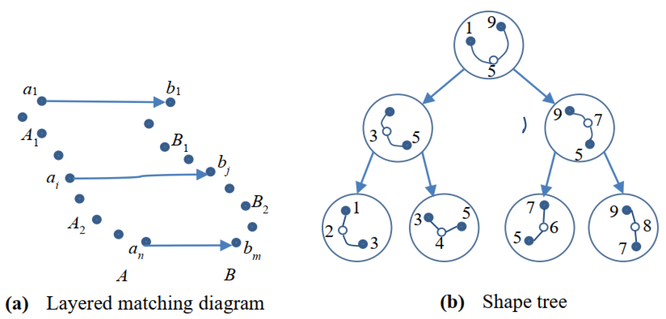
The selected midpoint ai divides the curve A into two parts: A1 = (a1, …, ai) and A2 = (ai, …, an). The layered description of curve A is recursive (i.e., the layered description of curve A consists of the relative position of L(ai|a1, an) and a layered description of A1 and A2). The layered description can be characterized by a binary tree, and the binary tree representation of the curve is referred to as a shape tree, as shown in Figure 9. The root node of the shape tree describes the position L(ai|a1, an) of the midpoint ai in the curve A relative to a1 and an, the left child node describes the position of the intermediate node in A1 relative to a1 and an, and the right child node describes the position of the intermediate node in A1 relative to a1 and an. For the subcurve , where p, q is the position of the first and last endpoints of the subcurve , the midpoint is selected as ak (k = ), and the corresponding subnode is described as . The layered description is sequentially performed until = p, and the shape tree is established.
The subtree rooted at a node represents the shape tree of the subcurve. Each node on the shape tree records the relative position of the midpoint of the curve and the first and last sampling points. The bottom node of the shape tree represents the relative positions of three consecutive points on the curve, and these nodes contain local geometric information, such as the relative position of the midpoint and adjacent sampling points.
Curve A, with the first and last sampling points, can recursively reconstruct the curve according to the shape tree. Placing the initial points at any position is equivalent to performing a translation, rotation, and scale transformation on curve A. Thus, the layered matching algorithm is invariant to translation, rotation, and scale transformation.
4.2.2. Improved Layered Elastic Matching
Matching is performed between two open curves A and B. First, we establish the shape tree of curve A and then find its corresponding relationship on curve B to make the minimum deformation error between curve B and curve A. The process of matching is described below.
For the two to-be-matched curves and , let correspond to and to . The midpoint of the shape tree of A divides the curve into two parts and . are sequentially made as the midpoint of B, and divides the curve B into two parts, and corresponding to and , respectively. If the point is such that the similarity of and , the similarity of and and the weighted similarity of the relative positions between the two midpoints and in the two curves leads the sum to its minimum, the minimum similarity s is taken as the final similarity between A and B. According to the similarity between A and B, the similarity calculation between the subcurves and can be calculated according to the following optimal recursion equation:
where represents the relative position error of the midpoint between A and B, and is the weighting factor.
We use different weights for different nodes on the shape tree to represent the degree of the deformation. In this study, the weighting factor is determined according to the length of the curve. For the deformation with the longer distance between the relative position of the midpoint and the first and last sampling points, a higher weighting factor is assigned, and the reverse is even smaller.
Since we use the Bookstein coordinate system to represent the relative positional relationship of the three points, the point on the system is considered to be equivalent to the point on the morphospace [26]. Therefore, the relative position error of the midpoint is calculated by the Procrustes distance [27]. For the two points of the Bookstein coordinates and we first map to according to Equation (4):
where
And their Procrustes distance:
The following discussion is about the default condition of when there are only two sampling points in A or B. A curve with only two sample points is equivalent to a line segment, and the cost for matching is zero when they are matched. When the length of one-line segment and another separable curve is determined, the matching cost increases as the length of the separable curve increases, and the cost decreases when the length decreases.
Affected by its attitude, the surface of the human face undergoes some deformation, and different weights of curve similarity in different areas should be given for weighted fusion. The weight of the forehead area is increased, and the weight of the mouth and eye area is decreased. The weight calculation is shown in Equation (7):
where i is the serial number of the radial curve and the area where the radial curve located is the empirical value. Combining the results from six radial curves’ matching, the layered human face matching similarity is:
where is the layered matching similarity obtained from the comparison between the radial curve i on the test face and the corresponding radial curve on the face that is to be matched. By assigning different weights to different curves, the method overcomes the influences from attitude changes.
4.2.3. Point-Distance Information Fusion
The characteristic curve extracted from the human face is approximately a two-dimensional curve, so a layered matching algorithm is used for matching. However, some three-dimensional spatial information will be lost in this matching, which will have a certain influence on the recognition rate. To avoid this, it is necessary to extract the useful points of the curve and establish a point-to-point correspondence of the face curve. Using the Euclidean distance from each sampling point to the nose-tip for matching can effectively compensate for the loss of space information in the layer matching algorithm.
Since any point on the corresponding reference curve of each radial curve has a flag containing the sampling point, it is necessary to obtain the flag indicating whether the sampling point is available at the corresponding position before we perform the feature comparison:
That is, when point a on the test face and point b on the face to be matched are both available (the values are both 1), the pair of sample points participate in the comparison. Thus, assuming that the total number of samples of the radial curve i on each face is , we can obtain by Equation (9), which are the total available pairs of sampling points. If the distance between sampling point and the nose-tip point on the radial curve i of the face to be matched is , and the distance between the sampling point and the nose-tip point on the radial curve i of the test face is , then the feature similarity of each radial curve is defined as follows:
4.3. Similarity Calculation
For a set with face models of N, a layered matching similarity vector and the point-distance similarity vector are obtained. Two similarities are fused, and the two vectors are normalized; namely:
where . Normalized similarity vectors and thus are obtained, and the final similarity is their weighted sum. Since the layered matching similarity has better recognition performance than the point-distance matching similarity, the weight of the layered matching similarity is set to 0.6; the weight of the point-distance matching similarity is 0.4. The corresponding model with minimum similarity is the recognition results.
5. Experimental Results and Analysis
The experimental environment in this paper is shown in Figure 10 and is composed of a projector, camera, and computer. Both the camera and the projector are connected to the computer. The projector is a product of SHARP, with a resolution of 1280 × 720 and a brightness of 2000 lumens; it is lightweight and small-sized and thus suitable for our measurement environment. The camera is powered by Canon, with a resolution of 1920 × 1080. It is easy to place in a variety of measurement environments. The Central Processing Unit (CPU) model of the computer is Core i7-8550U, and the software used in this experiment is MATLAB R2018a.
In this experiment, 60 sets of images is collected in the natural light and darkness, and the different poses of 30 faces is tested. The background of the image is a white wall. A neutral face of each person is selected as the library set, and the remaining faces are used as a test set, forming an all vs. neutral experiment.
The 3D face reconstruction effect is better when the number of projected stripes is 64. Then, a set of four-step phase-shift diagrams are generated by the computer, as shown in Figure 11. The four-step phase-shift method is used to solve the wrapped phase value of each point in the image from the deformed stripe image, and the face wrapped phase diagram is obtained, as shown in Figure 12. The optimized branch cutting method is used to obtain the unrolled phase diagram of the object, and the 3D face image is reconstructed according to the phase height relationship, as shown in Figure 13. Figure 14 shows the reconstructed 3D face images in various postures.
When the layered matching is used for rank recognition alone, the recognition rate is 91.5%. Additionally, when the point-distance matching is used for rank recognition alone, the recognition rate is 76.5%. The layered elastic matching contains the local and global features of the curve, but since the method only uses the two-dimensional coordinate information of the sampling points and discards their one-dimensional information, the recognition rate is not ideal. The point-distance matching further uses the spatial distance of the sampling points relative to the nose-tip point. The recognition rate here may be lower, but it retains the spatial three-dimensional information well, which helps in the shortcomings of layered elastic matching. In this paper, we use a combination of point-distance matching and the layered elastic matching and obtain a higher recognition rate. The cumulative match characteristic (CMC) curves of the three experiments are shown in Figure 15.
To compare the performance of the face recognition method based on grating projection, we compare this method with other methods. Table 2 lists the recognition rates and speeds for iterative closest point (ICP), subspace pursuit (SP) and local binary pattern (LBP). It can be seen that the recognition rate of this method is higher, and the speed is faster, and it has better recognition performance.
Table 3 shows the identification of the method in this paper under different lighting conditions. Among the 120 three-dimensional face images with different facial attitudes under natural light, 116 images are accurately identified with a recognition rate of 96.67%. The rate has been dropped by 0.82% compared to the recognition in the dark environment. The recognition rate in both natural light and dark environment is above 90%, which indicates that the 3D face recognition method based on grating projection in this study has little influence from natural light.
6. Conclusions
Applying face recognition technology to the perception system of security robots can improve the efficiency of face recognition in intelligent security robots. With the help of the Internet of Things and the big data environment, we propose a new method for face recognition for intelligence security in this paper. First, a four-step phase-shifted fringe pattern is generated by a computer and transmitted to a projector. Then, it is projected onto the background surface and the surface of the object to be measured. Second, the camera obtains the background fringe pattern and the deformed fringe pattern separately and transmits them to the computer to solve the wrap phase value with the four-step phase-shift method. Then, the computer obtains the unwrapped phase value through an optimized Goldstein branching method and finds the height with the phase-to-height transformation formula, and thus reconstructs a 3D face image. Next, the system extracts the side contour line and the horizontal contour line and other radial curves from the nose-tip point on the face and performs improved layered matching and point-distance matching on different curves. Finally, it assigns two degrees of matching to different weights for a weighted fusion to find the total similarity for the 3D face recognition. This method requires a relatively simple set of equipment which includes only a computer, a projector, and a camera. As the experiments above showed, compared to other algorithms such as ICP, SP, and LBP, this method has a relatively higher recognition rate (97.10%) on human faces with a faster speed of 2.81 s. Calculations show the method is robust to attitude, illumination, and noise and achieves a better recognition performance. It can be applied to smart cities [30] and civil security where intelligent security robots with efficient face recognition functions in the big data environment can be considered as innovations of the traditional security industry and public safety services. In the future, we hope to improve the face recognition rate and the resolution of the facial expressions, enrich the users’ scenarios, and increase market acceptance.
Author Contributions
Conceptualization, Z.W. and X.Z.; methodology, Z.W. and X.Z. and P.Y.; software, X.Z.; validation, X.Z. and P.Y.; formal analysis, Z.W.; investigation, W.D.; resources, Z.W. and W.D.; data curation, Z.W.; writing—original draft preparation, Z.W. and X.Z.; writing—review and editing, X.Z., D.Z., and N.C.; supervision, Z.W. and N.C.; project administration, Z.W. and N.C.; funding acquisition, Z.W. All authors have read and agreed to the published version of the manuscript.
Funding
This research was funded by the Science and Technology Support Plan Project of Hebei Province, grant number 17210803D and 19273703D; The Science and Technology Spark Project of Hebei Seismological Bureau, grant number DZ20180402056; The Education Department of Hebei Province, grant number QN2018095.
Conflicts of Interest
The authors declare no conflicts of interest.
References
- Tome, P.; Fierrez, J.; Vera-Rodriguez, R.; Nixon, M.S. Soft biometrics and their application in person recognition at a distance. IEEE Trans. Inf. Forensics Secur. 2014, 9, 464–475. [Google Scholar] [CrossRef]
- Bah, S.M.; Ming, F. An improved face recognition algorithm and its application in attendance management system. Array 2019, 5, 100014. [Google Scholar] [CrossRef]
- Nguyen, T.T.; Slaughter, D.C.; Max, N.; Maloof, J.N.; Sinha, N. Structured light-based 3D reconstruction system for plants. Sensors 2015, 15, 18587–18612. [Google Scholar] [CrossRef] [PubMed] [Green Version]
- Manzo, M.; Pellino, S. Bag of ARSRG Words (BoAW). Mach. Learn. Knowl. Extr. 2019, 1, 50. [Google Scholar] [CrossRef] [Green Version]
- Manzo, M. Graph-based image matching for indoor localization. Mach. Learn. Knowl. Extr. 2019, 1, 46. [Google Scholar] [CrossRef] [Green Version]
- Jin, Y.; Wang, Z.; Chen, Y.; Wang, Z. The online measurement of optical distortion for glass defect based on the grating projection method. Optik 2016, 127, 2240–2245. [Google Scholar] [CrossRef]
- Hu, F.; Somekh, M.G.; Albutt, D.J.; Webb, K.; Moradi, E.; See, C.W. Sub-100 nm resolution microscopy based on proximity projection grating scheme. Sci. Rep. 2015, 5, 8589. [Google Scholar] [CrossRef] [Green Version]
- Takeda, M.; Ina, H.; Kobayashi, S. Fourier-transform method of fringe-pattern analysis for computer-based topography and interferometry. J. Opt. Soc. Am. 1982, 72, 156–160. [Google Scholar] [CrossRef]
- Liu, Z.; Zibley, P.C.; Zhang, S. Motion-induced error compensation for phase shifting profilometry. Opt. Express 2018, 26, 12632–12637. [Google Scholar] [CrossRef]
- Luo, J.; Wang, Y.; Yang, X.; Chen, X.; Wu, Z. Modified five-step phase-shift algorithm for 3D profile measurement. Optik 2018, 162, 237–243. [Google Scholar] [CrossRef]
- Takeda, M.; Mutoh, K. Fourier transform profilometry for the automatic measurement of 3-D object shapes. Appl. Opt. 1983, 22, 3977–3982. [Google Scholar] [CrossRef] [PubMed]
- Vezzetti, E.; Tornincasa, S.; Moos, S.; Marcolin, F.; Violante, M.G.; Speranza, D.; Buisan, D. 3D human face analysis: Automatic expression recognition. In Proceedings of the Biomedical Engineering, Innsbruck, Austria, 15–16 February 2016. [Google Scholar]
- Marcolin, F.; Violante, M.G.; Moos, S.; Vezzetti, E.; Tornincasa, S.; Dagenes, N.; Speranza, D. Three-dimensional face analysis via new geometrical descriptors. Adv. Mech. Des. Eng. Manuf. 2016, 747–756. [Google Scholar]
- Nonis, F.; Dagnes, N.; Marcolin, F.; Vezzetti, E. 3D approaches and challenges in facial expression recognition algorithms—A literature review. Appl. Sci. 2019, 9, 3904. [Google Scholar] [CrossRef] [Green Version]
- Dagnes, N.; Vezzetti, E.; Marcolin, F.; Tornincasa, S. Occlusion detection and restoration techniques for 3D face recognition: A literature review. Mach. Vis. Appl. 2018, 29, 789–813. [Google Scholar] [CrossRef]
- Besl, P.J.; McKay, N.D. A method for registration of 3-D shapes. In Proceedings of the Sensor Fusion IV: Control Paradigms and Data Structures, Boston, MA, USA, 30 April 1992. [Google Scholar]
- Pan, G.; Wu, Z.; Pan, Y. Automatic 3D face verification from range data. In Proceedings of the 2003 International Conference on Multimedia and Expo. ICME’03. Proceedings, Baltimore, MD, USA, 6–9 July 2003. [Google Scholar]
- Beumier, C.; Acheroy, M. Automatic 3D face authentication. Image Vis. Comput. 2000, 18, 315–321. [Google Scholar] [CrossRef]
- Samir, C.; Srivastava, A.; Daoudi, M. Three-dimensional face recognition using shapes of facial curves. IEEE Trans. Pattern Anal. Mach. Intel. 2006, 28, 1858–1863. [Google Scholar] [CrossRef] [PubMed]
- Berretti, S.; Bimbo, A.D.; Pala, P. 3D face recognition using isogeodesic stripes. IEEE Trans. Pattern Anal. Mach. Intel. 2010, 32, 2162–2177. [Google Scholar] [CrossRef] [Green Version]
- Gökberk, B.; İrfanoğlu, M.O.; Akarun, L. 3D shape-based face representation and feature extraction for face recognition. Image Vis. Comput. 2006, 24, 857–869. [Google Scholar] [CrossRef]
- Fan, H.; Ren, L.; Long, T.; Mao, E. A high-precision phase-derived range and velocity measurement method based on synthetic wideband pulse Doppler radar. Sci. China Inf. Sci. 2017, 60, 082301. [Google Scholar] [CrossRef]
- Goldstein, R.M.; Zebker, H.A.; Werner, C.L. Satellite radar interferometry: Two-dimensional phase unwrapping. Radio Sci. 1988, 23, 713–720. [Google Scholar] [CrossRef] [Green Version]
- Nagamine, T.; Uemura, T.; Masuda, I. 3D facial image analysis for human identification. In Proceedings of the 11th IAPR International Conference on Pattern Recognition, The Hague, The Netherlands, 30 August–3 September 1992. [Google Scholar]
- Křepela, M.; Zahradník, D.; Sequens, J. Possible methods of Norway spruce (Picea abies [L.] Karst.) stem shape description. J. Sci. 2005, 51, 244–255. [Google Scholar]
- Bris, A.L.; Chehata, N. Urban morpho-types classification from SPOT-6/7 imagery and Sentinel-2 time series. In Proceedings of the 2019 Joint Urban Remote Sensing Event (JURSE), Vannes, France, 2–24 May 2019. [Google Scholar]
- Bronstein, A.M.; Bronstein, M.M.; Kimmel, R. Expression-invariant representations of faces. IEEE Trans. Image Process. 2007, 16, 188–197. [Google Scholar] [CrossRef]
- Low, C.Y.; Teoh, A.B.J.; Ng, C.J. Multi-fold Gabor, PCA, and ICA filter convolution descriptor for face recognition. IEEE Trans. Circuits Syst. Video Technol. 2019, 29, 115–129. [Google Scholar] [CrossRef] [Green Version]
- Zhou, L.F.; Du, Y.W.; Li, W.S.; Mi, J.X.; Luan, X. Pose-robust face recognition with Huffman-LBP enhanced by divide-and-rule strategy. Pattern Recognit. 2018, 78, 43–55. [Google Scholar] [CrossRef]
- Wang, Z.; Huo, W.; Yu, P.; Qi, L.; Geng, S.; Cao, N. Performance evaluation of region-based convolutional neural networks toward improved vehicle taillight detection. Appl. Sci. 2019, 9, 3753. [Google Scholar] [CrossRef] [Green Version]
Figure 1.
General process of face recognition.

Figure 2.
Hardware system block diagram.

Figure 3.
Overall flowchart of software.

Figure 4.
Images with different stripes: (a) stripe number 32, (b) stripe number 64, (c) stripe number 128.
Figure 4.
Images with different stripes: (a) stripe number 32, (b) stripe number 64, (c) stripe number 128.

Figure 5.
Three-dimensional (3D) face images with different stripes: (a) stripe number 32, (b) stripe number 64, (c) stripe number 128.
Figure 5.
Three-dimensional (3D) face images with different stripes: (a) stripe number 32, (b) stripe number 64, (c) stripe number 128.

Figure 6.
Side contour of a human face.

Figure 7.
Horizontal contour of a human face.

Figure 8.
Characteristic curve.

Figure 9.
Schematic diagram of the layered matching method.

Figure 10.
Schematic diagram of the system.

Figure 11.
Four-step phase-shift fringe pattern with 64 fringes: (a) phase shift is 0, (b) phase shift is , (c) phase shift is , (d) phase shift is .
Figure 11.
Four-step phase-shift fringe pattern with 64 fringes: (a) phase shift is 0, (b) phase shift is , (c) phase shift is , (d) phase shift is .

Figure 12.
Wrapped phase diagram of a human face.

Figure 13.
Reconstructed 3D human face.

Figure 14.
3D face reconstructed in various poses.

Figure 15.
CMC curves between the two matching methods.

Figure 16.
Recognition performances of different algorithms in different attitudes.


Table 1.
Phase unrolling time comparison.
| Algorithm | Time | Unexpanded Region |
|---|---|---|
| Goldstein | 320 s | There is |
| Least squares | 2650 s | There is not |
| This method | 335 s | There is not |
Table 2.
Performance comparison among different face recognition methods.
| Method | Recognition Rate | Speed/s |
|---|---|---|
| ICP | 95.95% | 4.66 |
| SP | 90.42% | 3.34 |
| LBP | 89.73% | 4.89 |
| This Method | 97.10% | 2.81 |
Table 3.
Performance comparison among different light conditions.
| Light Condition | Recognition Rate | Speed/s |
|---|---|---|
| Natural Light | 96.67% | 2.36 |
| Darkness | 95.85% | 2.97 |
© 2020 by the authors. Licensee MDPI, Basel, Switzerland. This article is an open access article distributed under the terms and conditions of the Creative Commons Attribution (CC BY) license (http://creativecommons.org/licenses/by/4.0/).
Share and Cite
MDPI and ACS Style
Wang, Z.; Zhang, X.; Yu, P.; Duan, W.; Zhu, D.; Cao, N. A New Face Recognition Method for Intelligent Security. Appl. Sci. 2020, 10, 852. https://doi.org/10.3390/app10030852
AMA Style
Wang Z, Zhang X, Yu P, Duan W, Zhu D, Cao N. A New Face Recognition Method for Intelligent Security. Applied Sciences. 2020; 10(3):852. https://doi.org/10.3390/app10030852
Chicago/Turabian StyleWang, Zhenzhou, Xu Zhang, Pingping Yu, Wenjie Duan, Dongjie Zhu, and Ning Cao. 2020. "A New Face Recognition Method for Intelligent Security" Applied Sciences 10, no. 3: 852. https://doi.org/10.3390/app10030852
Note that from the first issue of 2016, this journal uses article numbers instead of page numbers. See further details here.