Nonlinear System Identification of an All Movable Fin with Rotational Freeplay by Subspace-Based Method

School of Aeronautic Science and Engineering, Beihang University, Beijing 100191, China
*
Author to whom correspondence should be addressed.
Appl. Sci. 2020, 10(4), 1205; https://doi.org/10.3390/app10041205
Submission received: 7 January 2020
/
Revised: 4 February 2020
/
Accepted: 5 February 2020
/
Published: 11 February 2020
(This article belongs to the Section Mechanical Engineering)
Abstract
:To interpret the nonlinear system identification of multi-degree-of-freedom vibrating structures with freeplay, an estimation procedure based on subspace method in time domain is developed in this paper. Two types of freeplay, namely, central freeplay and offset freeplay, are estimated. Besides, the frequency response function matrices of the underlying linear system and overlying linear system are identified. By considering an all movable fin from a portion of a supersonic flutter test platform containing freeplay on the rigid rotating motion, two series of numerical experiments are applied for demonstration. Results show that the proposed approach indicates a high and reliable recognition of freeplay regions and the nominal linear system. The limitations of the method in this study are also discussed.
1. Introduction
Nonlinearity is generic in nature, and linear behavior is an exception [1]. Nonlinear vibrating behaviors have been reported in numerous pieces of engineering literature. Some self-excited nonlinear vibrations may lead to a catastrophic disaster, such as the nonlinear flutter in aerospace engineering and the chatter vibrations in manufacture. A few series of literature have discussed the chatter prediction and avoidance as earlier by Fofana [2,3,4], then followed by Urbikain [5,6,7,8]. Moreover, the summary could be found in the recent review [9]. In aerospace engineering, as studied by Tian et al. [10], the trapezoidal-plate-like structure may suffer from different types of nonlinear phenomena, such as jump, internal resonance, periodic, quasi-periodic, and chaotic motions. For a real-life structure with non-negligible nonlinearities, it is essential to provide the precise mathematical model to perform accurate and reliable predictions of the structure’s dynamic behavior. Therefore, experimental testing and system identification still play a key role because they help the structural dynamicist to reconcile numerical predictions with experimental investigations [1].
The last several decades have witnessed an increasing interest in the system identification of nonlinear mechanical structures for either academic researches or industry applications. A lot of methodologies were well-established through a variety of studies, such as restoring force surface method [11], NARMAX (nonlinear autoregressive moving average with exogeneous inputs) modeling [12,13], the Hilbert transform [14,15], and Volterra series [16]. For more details of developments and advances on the topic of nonlinear system identification in structural dynamics, readers can refer to the reviews proposed by Kerschen et al. [1] and later by Noël [17]. However, these methods were difficult to apply to complicated structures with more than one nonlinearities. On the other hand, it is difficult to apply the identified mathematical model directly in the control field.
With the development of system identification and control theory, nonlinear black-box modeling, like the Hammerstein–Wiener model, was proposed and widely used in control of the nonlinear system. A variety of identification methods were developed to estimate the nonlinear and linear model [18,19,20,21,22]. However, the establishment of the black-box model is based on data alone, lacking physical insight. This is a very ambitious objective knowing that nonlinearity may be caused by many different mechanisms and may result in a plethora of dynamic phenomena [1].
Recently, two types of feedback formulation on nonlinear system identification were developed, namely, reverse path (RP) method and nonlinear identification through feedback of the output (NIFO) method. Bendat [23] first introduced the RP method to a single-degree-of-freedom (SDOF) system and by Rice [24] to a multi-degree-of-freedom (MDOF) system. However, the requirement of exciting all the measured DOF was the obstacle to extensive applications for the RP method. Then, Richards and Singh [25] proposed the conditioned reverse path (CRP) method to overcome this limitation, but with more complicated RP formulation and more substantial computational burden.
Another type of feedback formulation is the NIFO method put forward by Adams and Allemang [26], who introduced a least-squares parameter estimation method to decouple the linear and nonlinear parameters during the nonlinear identification of a multi-input, multi-output (MIMO) system. Then, the subspace-based identification methods were introduced to the identification of nonlinear mechanical systems by taking advantage of this kind of nonlinear feedback interpretation. Marchesiello and Garibaldi [27] proposed the time-domain nonlinear subspace identification (TNSI) method firstly and Noël and Kerschen [28] developed the counterpart frequency-domain nonlinear subspace identification (FNSI) method. Then, a comparison between the capabilities of TNSI and FNSI was addressed by Noël [29] considering a series of numerical experiments towards a nonlinear SmallSat spacecraft along with stochastic analysis.
Smooth structural nonlinearities were chosen as demonstrations of system identification methods. However, the capability of identifying non-smooth nonlinearities was seldom discussed. As one typical non-smooth structural stiffness nonlinearity, freeplay has often been witnessed in joints, bearings, hinges, and contact surfaces due to the manufacturing tolerance, wearing and tearing, or impacting. In practice, it is sometimes difficult to measure the actual gap directly. Furthermore, the nominal linear system of structure with freeplay plays an essential rule in the later structural and dynamic analysis since most of the analysis is performed under linear assumptions in practical engineering. To obtain an insight into the nonlinear behaviors of a structure with freeplay, both the nominal linear system and freeplay parameters have to be accurately estimated for better understanding. Wu et al. exploited the Hilbert transform [30] and CRP [31] method to freeplay identification. Noël [29] also addressed the identification of clearance. TNSI had been utilized on a 5-DOF structure with a one-side freeplay by Marchesiello [32]. However, little attention has been paid to the identification of freeplay with offset, which occurs more generally in real-life structures. Moreover, the existence of freeplay divides the original nonlinear system into three linear systems into different regions, and there remains a paucity of investigations on identifying them.
In the present paper, we perform a series of numerical experiments on an all movable fin considering two types of rotational freeplay. Both the modal parameters of the nominal linear system and nonlinear coefficients will be estimated by the subspace-based method. Subspace identification techniques are built upon the reformulation of the state-space relations Equation (4) in a matrix form [29]. There are several advantages of the subspace-based method. First, the approach can naturally deal with MIMO systems and has been successfully applied to a wide variety of real-life systems in control or biomedical as powerful identification tools [29]. Because the method identifies the input-state-output models instead of input-output models. Moreover, the robustness and high numerical performance of the method are guaranteed by making use of the geometric framework and numerical linear algebra decompositions. Therefore, the subspace system identification is a non-iterative method.
The paper is organized as follows. Section 2 briefly introduces the methodology of the TNSI method. The all movable fin is described in Section 3, along with its finite element model and reduced-order model. Furthermore, the definition of the underlying linear system and overlying linear system, and the description of two typical kinds of freeplay are also detailed. Section 4 details the identification of the all movable fin with either central freeplay or offset freeplay in its pitch degree of freedom. The performance of the TNSI method for estimating freeplay is also discussed. The frequency response function (FRF) matrix of both the underlying and overlying linear system of the nonlinear all movable fin were identified during these two sets of numerical experiments. Finally, Section 5 summarizes the conclusions.
2. Nonlinear Subspace Identification of Mechanical Systems
The system identification of a nonlinear mechanical system contains three steps: nonlinearity detection, characterization, and parameter estimation as summarized by Kerschen et al. [1]. However, detection and characterization of nonlinearity are not extended in the paper. The TNSI method discussed in this study is associated with the parameter estimation procedure and to estimate the FRF matrix of the nominal linear system together with the corresponding nonlinear coefficients.
2.1. State-Space Nonlinear Feedback Description
The governing equation of vibration of the nonlinear mechanical system under generalized coordinates is
where , , and are the linear mass, damping, and stiffness matrices, respectively. The superscript m means the nonlinear mechanical system is modeled by an m-DOF finite-element (FE) model. and are the generalized external force and displacement vectors, respectively. The nonlinear components are modeled by a lumped form that contains n nonlinearities in the system. is the mathematical description of the i-th nonlinearity and needs to be known previously. The location of the j-th nonlinearity is specified by a vector , the element of which is 0, 1, or . The unknown nonlinear coefficient is .
As subspace methods can obtain an identified state-space model, the second-order vibrating equation in Equation (1) is transformed into a first-order state-space description for better understanding. Defining the state vector and moving the nonlinear term to the right-hand side by considering the feedback interpretation [26] as shown in Figure 1, the dynamic equations are recast into
where the subscript indicates the continuous-time system; superscript stands for extended; , , , and are the state, extended input, output, and extended direct feed-through matrices, respectively; and N = 2 m. The extended input vector is .
The transform between state-space and physical-space model is
Equation (2) describe a continuous-time state-space system. However, in practice, the excited and observed signals of a vibrating system are measured by discrete-time sampling. A discrete-time translation of Equation (2) is introduced, and the discrete-time state-space system is
where k is the sampled time and subscript represents discrete-time.
2.2. Subspace System Identification
As the nonlinear vibrating equation can be recast into a discrete-time state-space system as presented in Equation (4), the identified state-space model within a similarity transformation can be obtained using the subspace-based method. The procedure of subspace system identification is briefly given. The identification problem statement of subspace identification algorithms is as follows, for a given s measurements of the input and the output generated by the unknown system of order N, to determine the order N of the unknown system and the system matrices , , , and up to within a similarity transformation [33]. In the time domain, the output Hankel matrix is defined as
where i is an user-defined index, l is typically equal to , and s is the number of data sample. The subscript p and f stand for past and future, respectively. Similarly, the extended input block Hankel matrix is
Then the time-domain output-state-input matrix equation Equations (4) is rewritten as follows by taking account of extended observability matrix and the lower-block triangular Toeplitz matrix .
where is the state sequence, and and are defined as
To estimate the observability matrix, the terms in Equation (7), depending on , are eliminated using an oblique projection with the symbol as
where .
Different left and right user-defined weighting matrices are applied to the oblique projection induce various of subspace algorithms, such as N4SID [34], MOESP [35], and CVA [36]. Then, the singular value decomposition (SVD) of weighted oblique projection, from which the order of estimated model and the estimated observability matrix are determined. Finally, the estimated matrices and are derived. Readers can refer to [33] for more detailed computation procedures.
2.3. Estimation of Underlying Linear System and Nonlinear Coefficients
As mentioned previously, the estimated matrices and are within a similarity transformation. Therefore, the structural parameters can not be extracted directly from these matrices. Fortunately, it is not necessary to compute the similarity transformation matrix that the system parameters can be obtained based on an invariant matrix called extended FRF matrix defined as
where the subscript stands for extended. Here, only in Equation (10), is the imaginary unit and is the angular frequency. The invariance property of the extended FRF matrix up to the similarity transformation has been proofed [27]. However, the identified matrices are discrete-time state-space model and need to transform to the corresponding continuous-time system. In general, the zero-order hold assumption is considered and the transformations are
One should point out that, it is difficult to maintain zero-order-hold assumption if the sample frequency is too low. Then, the bilinear transformation should be performed while mapping the discrete-time matrices to continuous-time domain [28].
Assuming the FRF matrix of underlying linear system is defined likely as Equation (10), the relationship between and is
where
The underlying linear system and the nonlinear coefficients can be identified from Equation (12).
3. Modeling of an All Movable Fin with Rotational Freeplay
3.1. Freeplay Nonlinearity
Freeplay nonlinearity is a special case of piecewise linear stiffness nonlinearity that the inner stiffness is zero. There are often two typical freeplay in a real structure, namely, central freeplay and offset freeplay. The central freeplay, with the two limits of the freeplay region being symmetrical as shown in Figure 2a, is defined as
where q is the generalized displacement and is the generalized restoring force. is the outer stiffness of central freeplay and the subscript stands for outer. d is the limit of gap, and the freeplay region is .
Because of the existence of freeplay, the nonlinear vibrating system has discontinuous nonlinear stiffness and becomes three piecewise linear systems with different regions. For nonlinear systems with freeplay, the nominal system is the overlying linear system (OLS), that is the system without freeplay ( as shown in Figure 2a) and full stiffness [37]. Moreover, the underlying linear system (ULS) possessing zero stiffness ( in Figure 2a) on the source of freeplay is also important for the nonlinear mechanical system. As for nonlinear aeroelastic analysis, the characteristics of the underlying linear system offer an additional reference to the nonlinear behavior and are paid more attention.
The restoring force of the offset freeplay is depicted in Figure 2b, whereby there is a shift on the generalized displacement, as defined in Equation (15). As freeplay generally occurs due to wear and to loosen of components, it is not necessarily centered [37]. and are the left and right limits of the gap, respectively, and the freeplay region is . The underlying linear system and overlying linear system for a system with offset freeplay can also be defined similarly to the one with central freeplay.
3.2. Description of the All Movable Fin
The numerical experiments of nonlinear system identification were carried out on a supersonic flutter test platform as shown in Figure 3. The test platform was assembled on a rigid base with an all movable fin connecting by an elastic beam. Based on the convenience of performing the ground vibration tests (GVTs) and the compatibility requirements of mounting on the side walls of the wind tunnel, the rigid base was designed with sufficient weight and stiffness. To simulate the installation environment of the fin, a rotating device was also considered inside the rigid base with rotating fixed. The base was made of steel while the all movable fin, specified as a skeleton-cover structure, was manufactured using aluminum-alloy. With several additional weights inside, the whole mass of the all movable fin is 3.20 kg. The size of the elastic beam was designed to meet the stiffness requirements, which was also made of steel.
The all movable fin was tested and identified by linear system identification techniques to obtain the natural frequency and mode shapes. Figure 4 presents the experimental set-up of GVTs performed using LMS Test.Lab. Burst random excitation was applied on the two selected nodes by a shaker, separately. Furthermore, the displacements of four selected nodes were sampled by four laser sensors. The sampling frequency was set to 2000 Hz to avoid the bias of low-frequency sampling. Table 1 gives the natural frequencies and damping ratios of the first 2 modes of all movable fin up to 150 Hz of interests. The mode shapes of the first two modes are shown in Figure 5.
The finite-element (FE) model was established by MSC Nastran [38] and has been modified based on the test results of GVTs using FEMTools [39], an optimization software developed by Dynamic Design Solutions. Figure 6 is the FE model of the all movable fin and elastic beam. The white-colored component is the all movable fin, whereas the cyan-colored component is the elastic beam. To reduce computational burdens and achieve faster nonlinear calculations, the linear elements of the FE model were condensed using the modal synthesis technique. The whole FE model was reduced in terms of several elastic modes of all movable fin and two assumed modes involve the rigid bending and rotating motion of all movable fin. Freeplay nonlinearity was finally introduced to the rigid rotating DOF. The freeplay regions considered in this paper are listed in Table 2.
A 4–5th-order Runge–Kutta time integration was performed with the same sampling frequency of 2000 Hz as GVTs during the numerical investigation. The mechanical and electrical disturbances in measurements were considered by adding a 0–150 Hz white noise to the synthetic signals, and the noise–signal ratio was set to 2%.
4. Nonlinear Identification Based on Random Excitation
The nonlinear identification of the all movable fin based on the subspace algorithm was addressed in this section. In the first numerical experiment, a periodic random forcing was applied to the structure with central freeplay. The location of excitation was chosen as same as in GVTs. The responses of the four nodes corresponding to the GVTs were observed by direct time integration, which was performed on the reduced-order model under generalized coordinates description. The nonlinearity in the structure was thoroughly excited by a series of different excitation levels. A second investigation was aimed to freeplay with offset. Both ULS and OLS were identified during the two cases of nonlinear system identification, and the stabilization diagrams were applied to estimate the modal parameters.
4.1. Identification of Central Freeplay
As the TNSI method exploited directly Input–Output data in time-domain that will not suffer from leakage and aliasing for no need to transform to frequency-domain, a random noise forcing was applied perpendicularly on the all movable fin at the same exciting location in Figure 4. The excitation signal consisted of 60,000 points over 30 s and band-limited in 0–150 Hz of interests, and repeated 5 times at each excitation level. It also has been discussed in [29] that the transient response was generally found to yield improved results compared with the steady-state regime, especially in the estimation of the linear modal properties. The analysis was conducted using the output data in terms of generalized coordinates established by the modal synthesis method for straightforward identification of freeplay. Therefore, the excitation force has to transform into generalized forces as input data.
However, the accuracy of nonlinear system identification is conditional upon the selection of the mathematical forms introduced in Equation (1). In particular, the boundary of different subsystem regions in Figure 2 plays a key rule in freeplay nonlinearity and still remain a challenging task. First, user-defined multiple piecewise-linear functions with varying clearances are used to representing the nonlinearity to be identified. Then, the freeplay can be posterior, determined after the reconstruction of nonlinear restoring force established by the participation of the user-defined functions. In a detailed explanation, we can assume the relative displacement across the nonlinear connection is . Then, the displacement range of , i.e., , can be divided into l equally spaced intervals. Given the jth interval , the nonlinear form is defined as
where is the sign function.
Figure 7 shows the nonlinear coefficients estimated by Equation (12). All estimations of indicate that the limit of central freeplay lies at approximately . Then, the reconstruction of the nonlinear restoring force is performed based on the identified nonlinear coefficients and mathematical form , which is shown in Figure 8. However, it seems that dividing more intervals would not improve or even reduce the accuracy of identification, even though the estimated limits of the freeplay region are within an acceptable range. Therefore, a proper division of the displacement range is essential and the number of the interval l around 10 would lead a better estimation.
An alternative way to improve the accuracy is to narrow the displacement range of varying clearances and repeat a 2nd estimation. A further division of the range into 10 new sub-intervals based on the 1st estimation of nonlinear coefficient in Figure 7. The identified nonlinear coefficients in the range from to is presented in Figure 9a that a more precise estimate can be inferred, and the identified nonlinear restoring force is shown in Figure 9b, which meets the theoretical nonlinear restoring force with high consistency.
Then, the estimated FRF () of OLS was depicted in Figure 10. TNSI method gives a clear FRF of the OLS; however, FRF estimated by traditional linear method possesses a significant distortion with no observable peak on the contrary, which may lead to an incorrect estimation of modal parameters. Then, the stabilization diagrams computed by TNSI method indicate the natural frequency and the damping ratio of the overlying linear system in Figure 11 with the max modal order up to 20.
Different from the amplitude independence for the linear system, the dependence on amplitude or frequency of nonlinear behavior is one of the inherent properties of the nonlinear system. Therefore, numerical investigations on varying excitation levels were also considered while applying TNSI method. Figure 12a counted the distributions of nonlinear DOF in different phases as mentioned in Figure 2a. The estimated restoring force is depicted in Figure 12b. The estimations of the freeplay region are excellent; however, the estimation on outer stiffness is still required to be improved by repeating the same identifying procedure in a narrower range.
4.2. Identification of Offset Freeplay
Another series of numerical experiments of offset freeplay were carried out with similar simulating parameters as in the previous numerical experiment. The excitation was generated a Gaussian white-noise signal of 60,000 points in 30 s and band-limited in 0–150 Hz repeating 5 times. The analysis was also conducted in terms of generalized coordinates. The identification problem is complicated by the existence of offset in freeplay; however, it is still in reach with utilization of the TNSI method considering some adjustments and skills.
The selection of the mathematical forms is different from central freeplay because of the offset. The identification of the left limit and the right limit of the freeplay region are operated separately in two different sets of displacement ranges. Similar to the procedure of identifying central freeplay, the 1st two sets of ranges is based on the boundary of relative displacement response, i.e., and . The displacement ranges can likely be divided into and equally spaced intervals, respectively, where the subscripts − and + stand for negative and positive. Given the jth negative interval , the nonlinear form is defined as
Similarly, for the jth positive interval , the nonlinear form is
and the nonlinear terms is the summary of and .
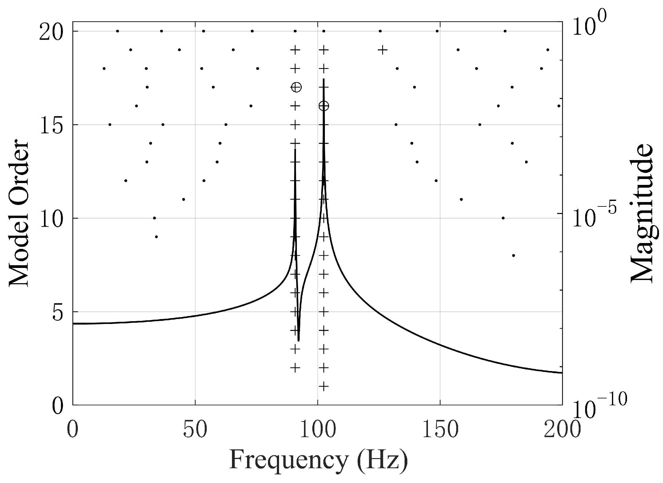
Figure 13 gives the magnitude of nonlinear force contributions identified by TNSI method when and . Both of the results indicate that the left limit of the freeplay region is around , whereas the right one is near to . The reconstruction of the nonlinear restoring force is plotted in Figure 14, indicating an accurate estimation of the inflection points in the offset freeplay. A same procedure is also repeated considering division of the narrowed ranges and to improve the results as the force contribution in Figure 15a and the nonlinear restoring force in Figure 15b. The modal parameters of OLS can still be extracted from the stabilization diagram in Figure 16.
The identified natural frequencies of OLS based on the two numerical experiments previously are summarized in Table 3.
5. Conclusions
(1) An identification methodology on a nonlinear system with central and offset freeplay was proposed and demonstrated in this paper. With the utilization of test data under random excitation force, both the underlying linear structure and overlying linear structure were estimated, with the company of estimated coefficients of the freeplay by exploiting the TNSI method. Furthermore, the identified state-space model can naturally be used in the control field.
(2) A series of numerical experiments were implemented. With comparison to the theoretical system, the estimated regions of either central or offset freeplay were accurate using the TNSI method. The capability of the present approach to identifying the offset freeplay indicates a more widely potential application to real-life structures. Combined with the modal synthesis technique, the TNSI method can also identify complicated MDOF structures.
(3) However, one limitation is that the outer stiffness of freeplay may shift depending on the division of response range. In the future, an experimental implementation of the TNSI method is in reach. However, a more robust integrated procedure based on TNSI needs to be developed on practical applications.
Author Contributions
Conceptualization, S.Y. and W.Z.; Data curation, W.Z.; Formal analysis, B.L.; Funding acquisition, Y.C. and W.Z.; Investigation, S.Y.; Methodology, S.Y.; Project administration, W.Z.; Resources, B.L.; Software, S.Y.; Supervision, Y.C.; Validation, Y.C. and W.Z.; Visualization, S.Y. and B.L.; Writing—original draft, S.Y.; Writing—review & editing, S.Y. and W.Z. All authors have read and agreed to the published version of the manuscript.
Funding
This research was funded by National Natural Science Foundation of China (grant number 11372023).
Conflicts of Interest
The authors declare no conflicts of interest.
Abbreviations
The following abbreviations are used in this manuscript:
| CRP | Conditioned reverse path |
| CVA | Canonical variate analysis |
| DOF | Degree of freedom |
| FRF | Frequency response function |
| MDOF | Multi-degree-of-freedom |
| MIMO | Multi-input, multi-output |
| MOESP | Multivariable output error state space |
| NARMAX | Nonlinear autoregressive moving average with exogeneous inputs |
| NIFO | Nonlinear identification through feedback of the output |
| N4SID | Numerical algorithms for subspace state space system identification |
| OLS | Overlying linear system |
| RP | Reverse path |
| SDOF | Single-degree-of-freedom |
| TNSI | Time-domain nonlinear subspace identification |
| ULS | Underlying linear system |
References
- Kerschen, G.; Worden, K.; Vakakis, A.F.; Golinval, J.C. Past, present and future of nonlinear system identification in structural dynamics. Mech. Syst. Signal Process. 2006, 20, 505–592. [Google Scholar] [CrossRef] [Green Version]
- Deshpande, N.; Fofana, M.S. Nonlinear regenerative chatter in turning. Robot. Comput.-Integr. Manuf. 2001, 17, 107–112. [Google Scholar] [CrossRef]
- Fofana, M.S. Sufficient conditions for the stability of single and multiple regenerative chatter. Chaos Solitons Fractals 2002, 14, 335–347. [Google Scholar] [CrossRef]
- Fofana, M.S. Delay dynamical systems and applications to nonlinear machine-tool chatter. Chaos Solitons Fractals 2003, 17, 731–747. [Google Scholar] [CrossRef]
- Urbikain, G.; López de Lacalle, L.N.; Campa, F.J.; Fernández, A.; Elías, A. Stability prediction in straight turning of a flexible workpiece by collocation method. Int. J. Mach. Tools Manuf. 2012, 54–55, 73–81. [Google Scholar] [CrossRef]
- Urbikain, G.; López de Lacalle, L.N.; Fernández, A. Regenerative vibration avoidance due to tool tangential dynamics in interrupted turning operations. J. Sound Vib. 2014, 333, 3996–4006. [Google Scholar] [CrossRef]
- Urbikain, G.; Campa, F.J.; Zulaika, J.J.; López de Lacalle, L.N.; Alonso, M.A.; Collado, V. Preventing chatter vibrations in heavy-duty turning operations in large horizontal lathes. J. Sound Vib. 2015, 340, 317–330. [Google Scholar] [CrossRef]
- Urbikain, G.; Olvera, D.; de Lacalle, L.L.; Elías-Zuñiga, A. Spindle speed variation technique in turning operations: Modeling and real implementation. J. Sound Vib. 2016, 383, 384–396. [Google Scholar] [CrossRef]
- Urbikain, G.; Olvera, D.; López de Lacalle, L.N.; Beranoagirre, A.; Elías-Zuñiga, A. Prediction Methods and Experimental Techniques for Chatter Avoidance in Turning Systems: A Review. Appl. Sci. 2019, 9, 4718. [Google Scholar] [CrossRef] [Green Version]
- Tian, W.; Yang, Z.C.; Zhao, T. Analysis of nonlinear vibrations and dynamic responses in a trapezoidal cantilever plate using the Rayleigh-Ritz approach combined with the affine transformation. Math. Probl. Eng. 2019, 1, 1–23. [Google Scholar] [CrossRef]
- Masri, S.F.; Caughey, T.K. A nonparametric identification technique for nonlinear dynamic problems. J. Appl. Mech. 1979, 46, 433–447. [Google Scholar] [CrossRef]
- Leontaritis, I.J.; Billings, S.A. Input-output parametric models for nonlinear systems, part I: Deterministic nonlinear systems. Int. J. Control 1985, 41, 303–328. [Google Scholar] [CrossRef]
- Leontaritis, I.J.; Billings, S.A. Input-output parametric models for nonlinear systems, part II: Stochastic nonlinear systems. Int. J. Control 1985, 41, 329–344. [Google Scholar] [CrossRef]
- Feldman, M. Nonlinear system vibration analysis using the Hilbert transform—I. Free vibration analysis method ‘FREEVIB’. Mech. Syst. Signal Process. 1994, 8, 119–127. [Google Scholar] [CrossRef]
- Feldman, M. Nonlinear system vibration analysis using the Hilbert transform—II. Forced vibration analysis method ‘FORCEVIB’. Mech. Syst. Signal Process. 1994, 8, 309–318. [Google Scholar] [CrossRef]
- Khan, A.A.; Vyas, N.S. Non-linear parameter using Volterra and Wiener theories. J. Sound Vib. 1999, 221, 805–821. [Google Scholar] [CrossRef]
- Noël, J.P.; Kerschen, G. Nonlinear system identification in structural dynamics: 10 more years of progress. Mech. Syst. Signal Process. 2017, 83, 2–35. [Google Scholar] [CrossRef]
- Narendra, K.S.; Gallman, P.G. An iterative method for the identification of nonlinear systems using a Hammerstein model. Autom. Control 1966, 11, 546–550. [Google Scholar] [CrossRef]
- Chang, F.H.I.; Luus, R. A noniterative method for identification using Hammerstein model. Autom. Control 1971, 16, 464–468. [Google Scholar] [CrossRef]
- Billings, S.A.; Fakhouri, S.Y. Non-linear system identification using the Hammerstein model. J. Syst. Sci. 1979, 10, 567–578. [Google Scholar] [CrossRef]
- Zhu, Y. Estimation of an N–L–N Hammerstein–Wiener model. Automatica 2002, 38, 1607–1614. [Google Scholar] [CrossRef]
- Crama, P.; Schoukens, J. Initial estimates of Wiener and Hammerstein Systems using multisine excitation. Instrum. Meas. 2001, 50, 1791–1795. [Google Scholar] [CrossRef]
- Bendat, J.S. Spectral techniques for nonlinear systems analysis and identification. Shock Vib. 1993, 1, 21–31. [Google Scholar] [CrossRef]
- Rice, H.J.; Fitzpatrick, J.A. A procedure for the identification of linear and nonlinear multi-degree-of freedom systems. J. Sound Vib. 1991, 149, 397–411. [Google Scholar] [CrossRef]
- Richards, C.M.; Singh, R. Identification of multi-degree-of-freedom nonlinear systems under random excitation by the “reverse path” spectral method. J. Sound Vib. 1998, 213, 673–708. [Google Scholar] [CrossRef]
- Adams, D.E.; Allemang, R.J. A frequency domain method for estimating the parameters of a nonlinear structural dynamic model through feedback. Mech. Syst. Signal Process. 2000, 14, 637–656. [Google Scholar] [CrossRef]
- Marchesiello, S.; Garibaldi, L. A time domain approach for identifying nonlinear vibration structures by subspace methods. Mech. Syst. Signal Process. 2008, 22, 81–101. [Google Scholar] [CrossRef]
- Noël, J.P.; Kerschen, G. Frequency-domain subspace identification for nonlinear mechanical systems. Mech. Syst. Signal Process. 2013, 40, 701–717. [Google Scholar] [CrossRef]
- Noël, J.P.; Marchesiello, S.; Kerschen, G. Subspace-based identification of a nonlinear spacecraft in the time and frequency domains. Mech. Syst. Signal Process. 2014, 43, 217–236. [Google Scholar] [CrossRef]
- Wu, Z.G.; Yang, N.; Yang, C. Identification of nonlinear multi-degree-of freedom structures based on Hilbert transformation. Sci. China-Phys. Mech. Astron. 2014, 57, 1725–1736. [Google Scholar] [CrossRef]
- Wu, Z.G.; Yang, N.; Yang, C. Identification of nonlinear structures by the conditioned reverse path method. J. Aircr. 2015, 52, 373–386. [Google Scholar] [CrossRef]
- Marchesiello, S.; Garibaldi, L. Identification of clearance-type nonlinearities. Mech. Syst. Signal Process. 2008, 22, 1133–1145. [Google Scholar] [CrossRef]
- Overschee, P.V.; Moor, B.D. Subspace Identification for Linear Systems: Theory-Implementation-Applications; Kluwer Academic Publishers: Dordrecht, The Netherlands, 1996; pp. 96–97. [Google Scholar]
- Overschee, P.V.; Moor, B.D. N4SID: Numerical algorithms for state space subspace system identification. In Proceedings of the World Congress of the International Federation of Automatic Control, IFAC, Sydney, Australia, 1 July 1993; pp. 361–364. [Google Scholar]
- Verhaegen, M. Identification of the deterministic part of MIMO state space models given in innovations form from input-output data. Automatica 1994, 30, 61–74. [Google Scholar] [CrossRef]
- Larimore, W.E. Canonical variate analysis in identification, filtering and adaptive control. In Proceedings of the 29th Conference on Decision and Control, Honolulu, HI, USA, 5–7 December 1990; pp. 596–604. [Google Scholar]
- Dimitriadis, G. Introduction to Nonlinear Aeroelasticity; John Wiley & Sons, Inc.: Chichester, UK; West Sussex, UK, 2017; pp. 264–266. [Google Scholar]
- MSC Nastran User’s Manual. Getting Started with MSC Nastran User’s Guide; MSC Software Co.: Santa Ana, CA, USA, 2012. [Google Scholar]
- Dynamic Design Solutions NV. Getting Started with FEMtools Version 3.7.1; Dynamic Design Solutions NV: Leuven, Belgium, 2014. [Google Scholar]
Figure 1.
The feedback interpretation of nonlinear vibrating system.

Figure 2.
The restoring force of freeplay.
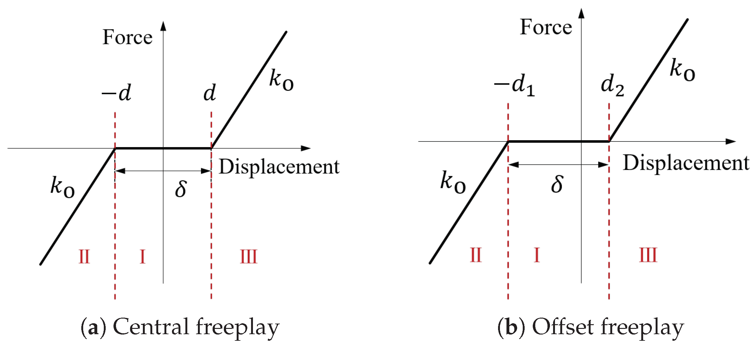
Figure 3.
The supersonic flutter test platform.
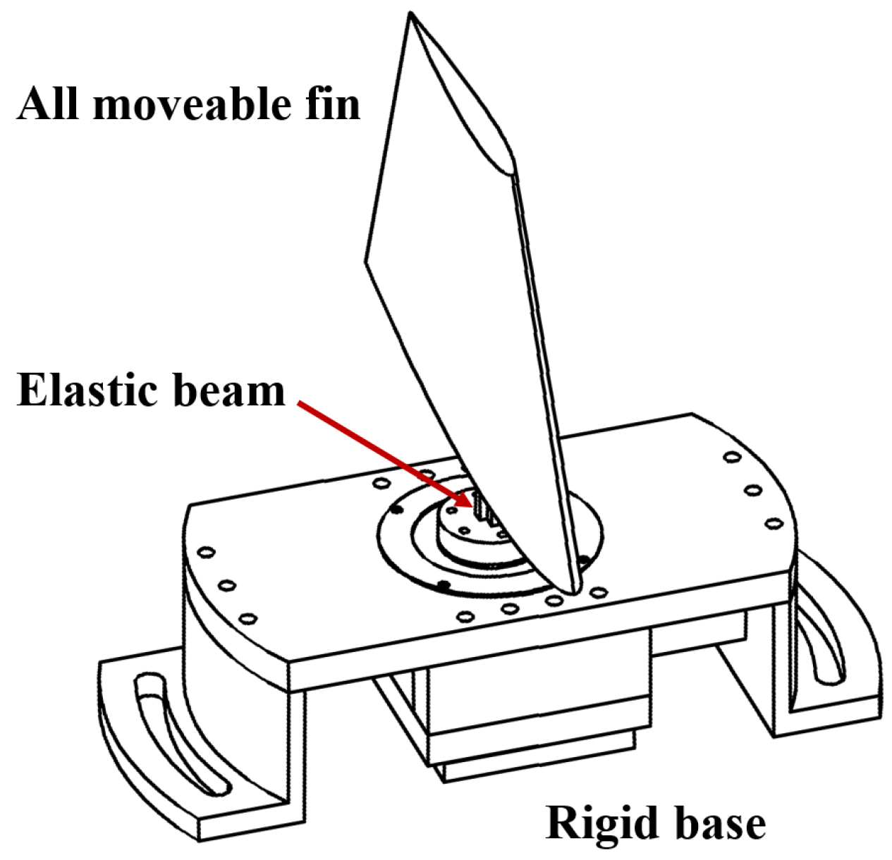
Figure 4.
The experimental set-up of ground vibration tests.

Figure 5.
The first 2 mode shapes of all movable fin.
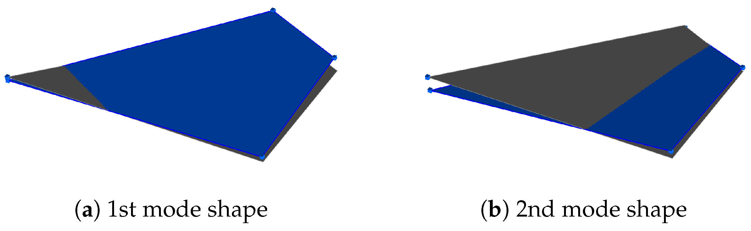
Figure 6.
The finite element model of the all movable fin and elastic beam.
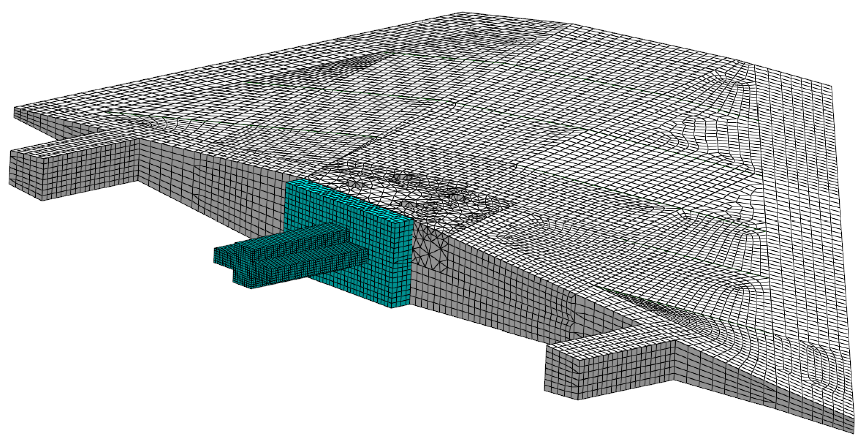
Figure 7.
The estimation of the nonlinear contribution of central freeplay using the 1st displacement range .
Figure 7.
The estimation of the nonlinear contribution of central freeplay using the 1st displacement range .
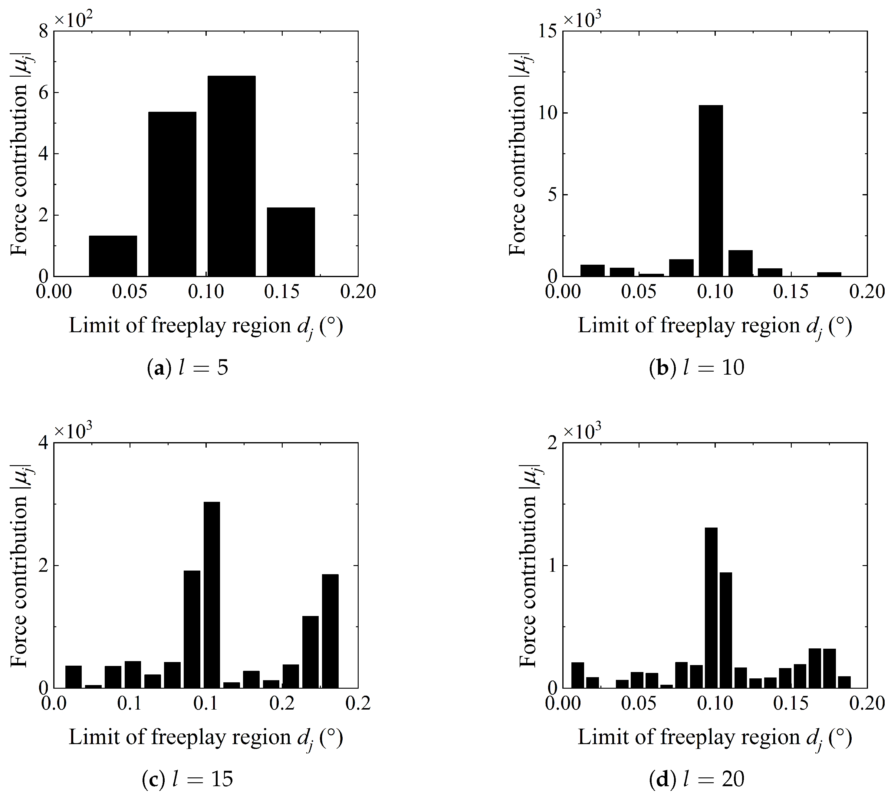
Figure 8.
The reconstruction of restoring force of central freeplay under different divisions.
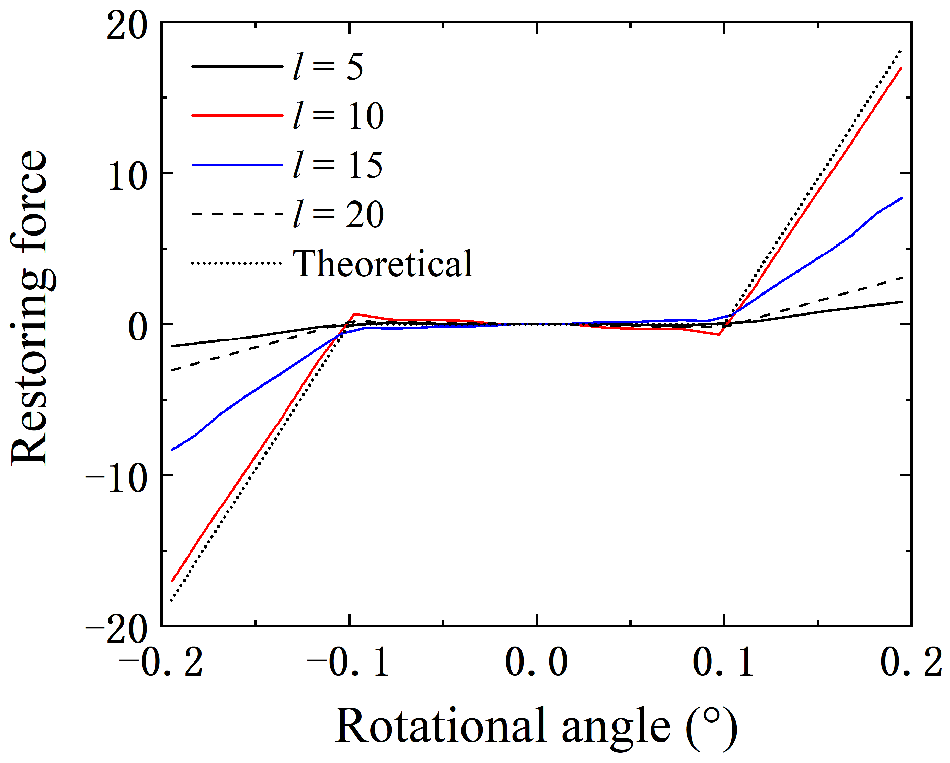
Figure 9.
The identification of central freeplay using the 2nd displacement range .
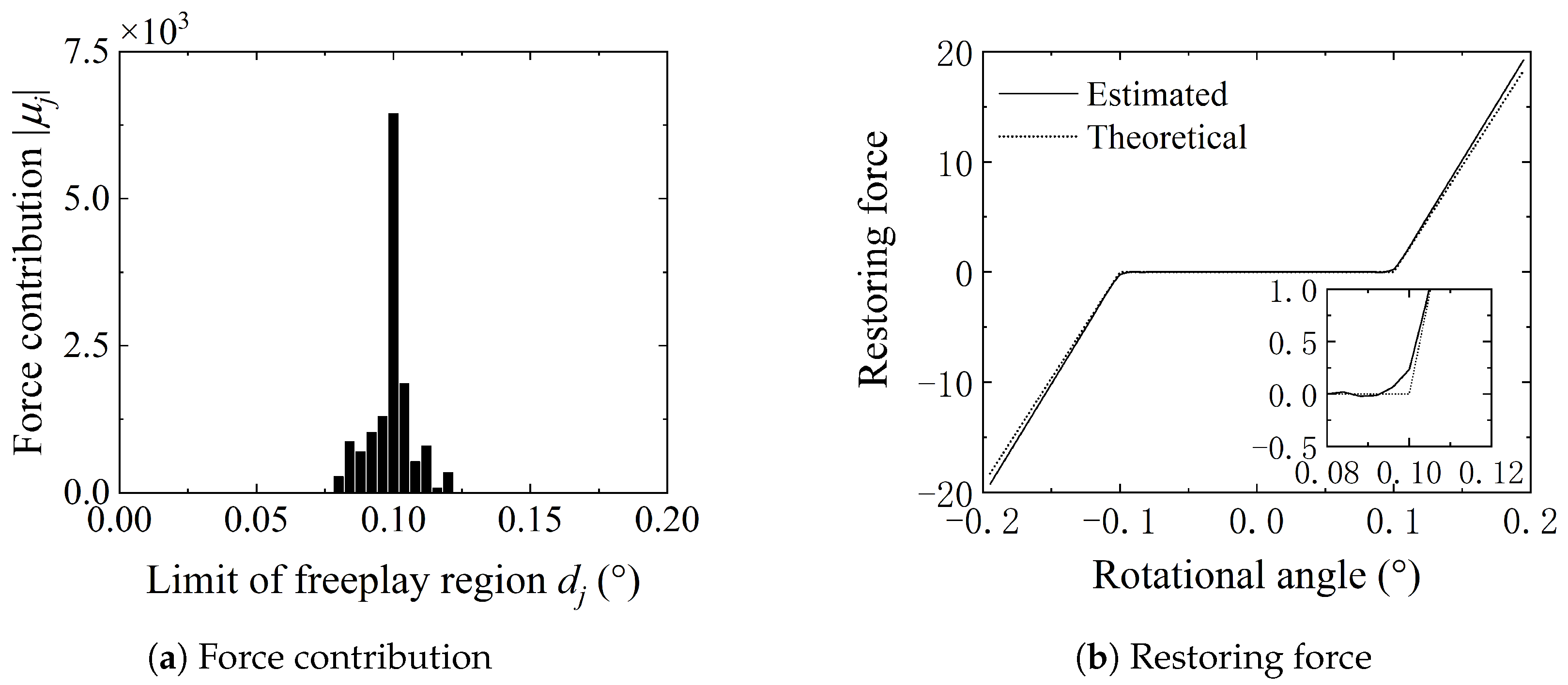
Figure 10.
The estimated frequency response function (FRF) () of overlying linear system (OLS) using time-domain nonlinear subspace identification (TNSI) method.
Figure 10.
The estimated frequency response function (FRF) () of overlying linear system (OLS) using time-domain nonlinear subspace identification (TNSI) method.
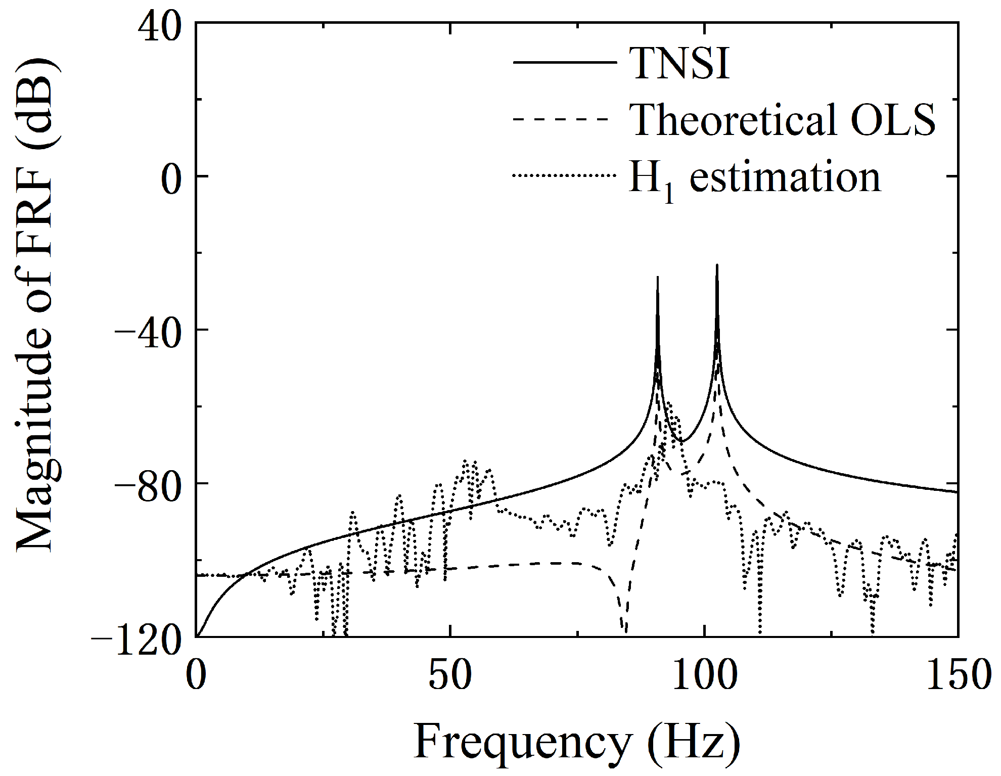
Figure 11.
Stabilization diagram of OLS of central freeplay computed by TNSI method using the estimated FRF (). (Dot: Not stable in frequency; Circle: Stable in frequency; Cross: Stable in frequency and damping.).
Figure 11.
Stabilization diagram of OLS of central freeplay computed by TNSI method using the estimated FRF (). (Dot: Not stable in frequency; Circle: Stable in frequency; Cross: Stable in frequency and damping.).
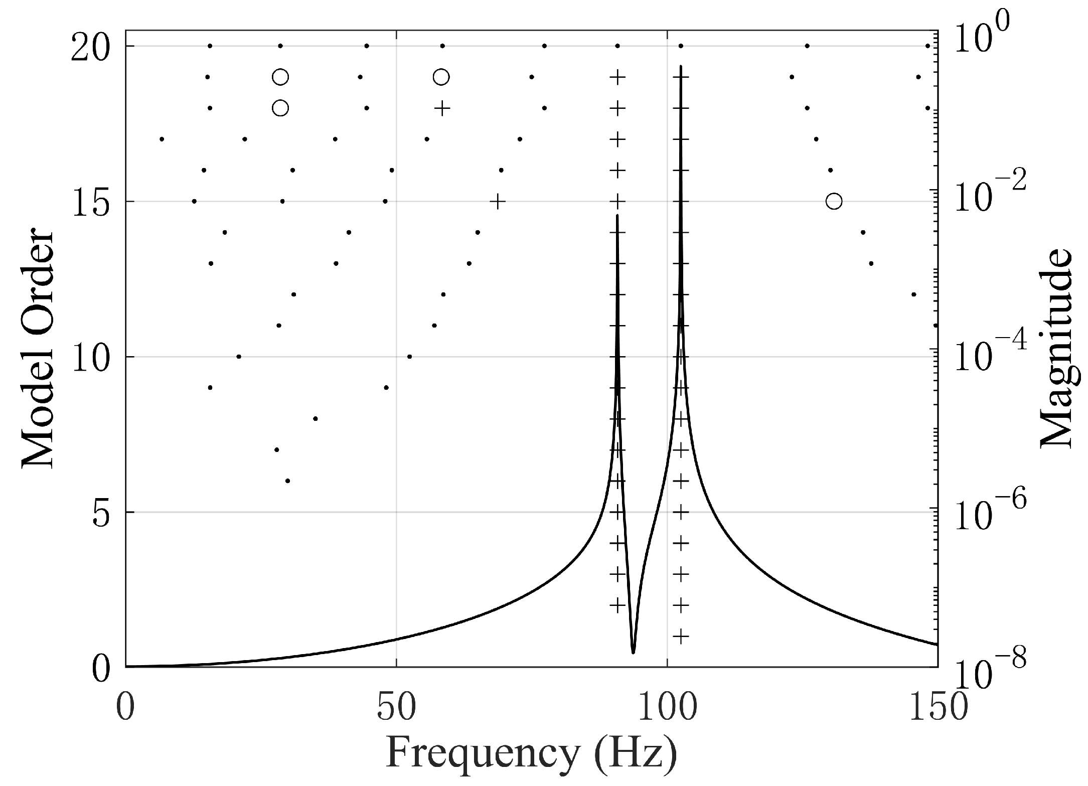
Figure 12.
The nonlinear identification of different excitation levels.
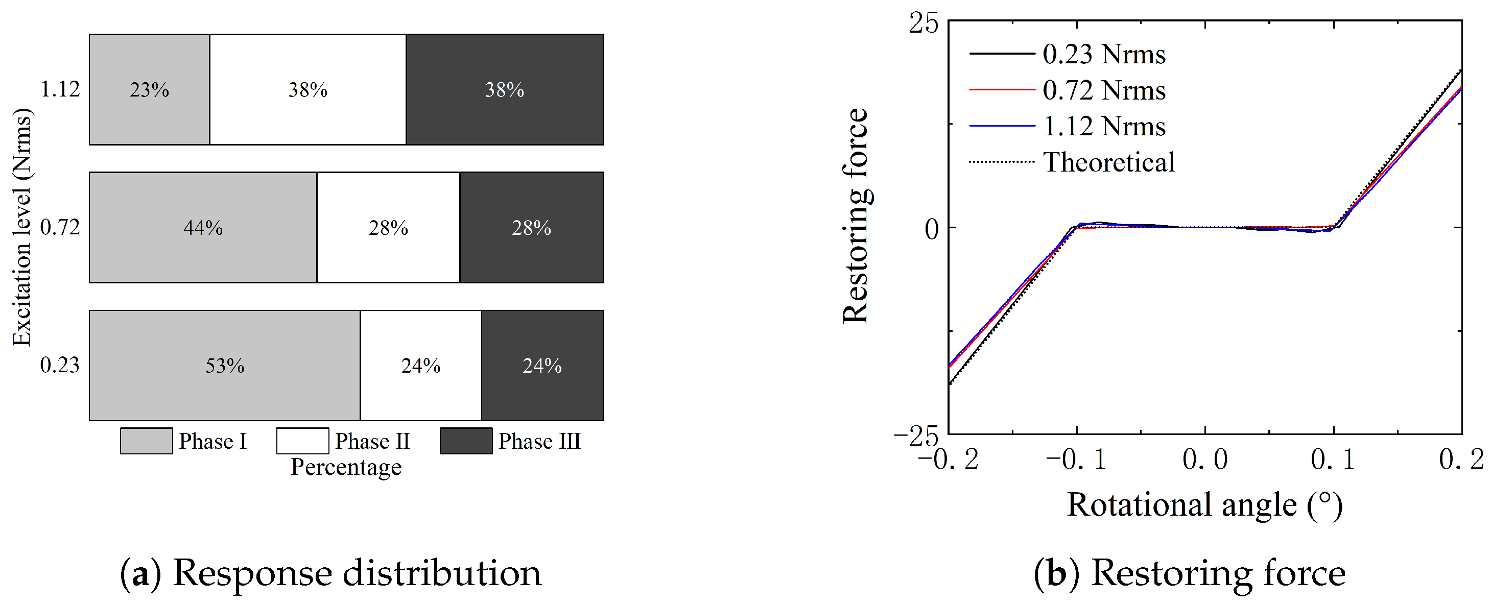
Figure 13.
The identification of offset freeplay using the 1st displacement range .

Figure 14.
The nonlinear restoring force of offset freeplay under different divisions.
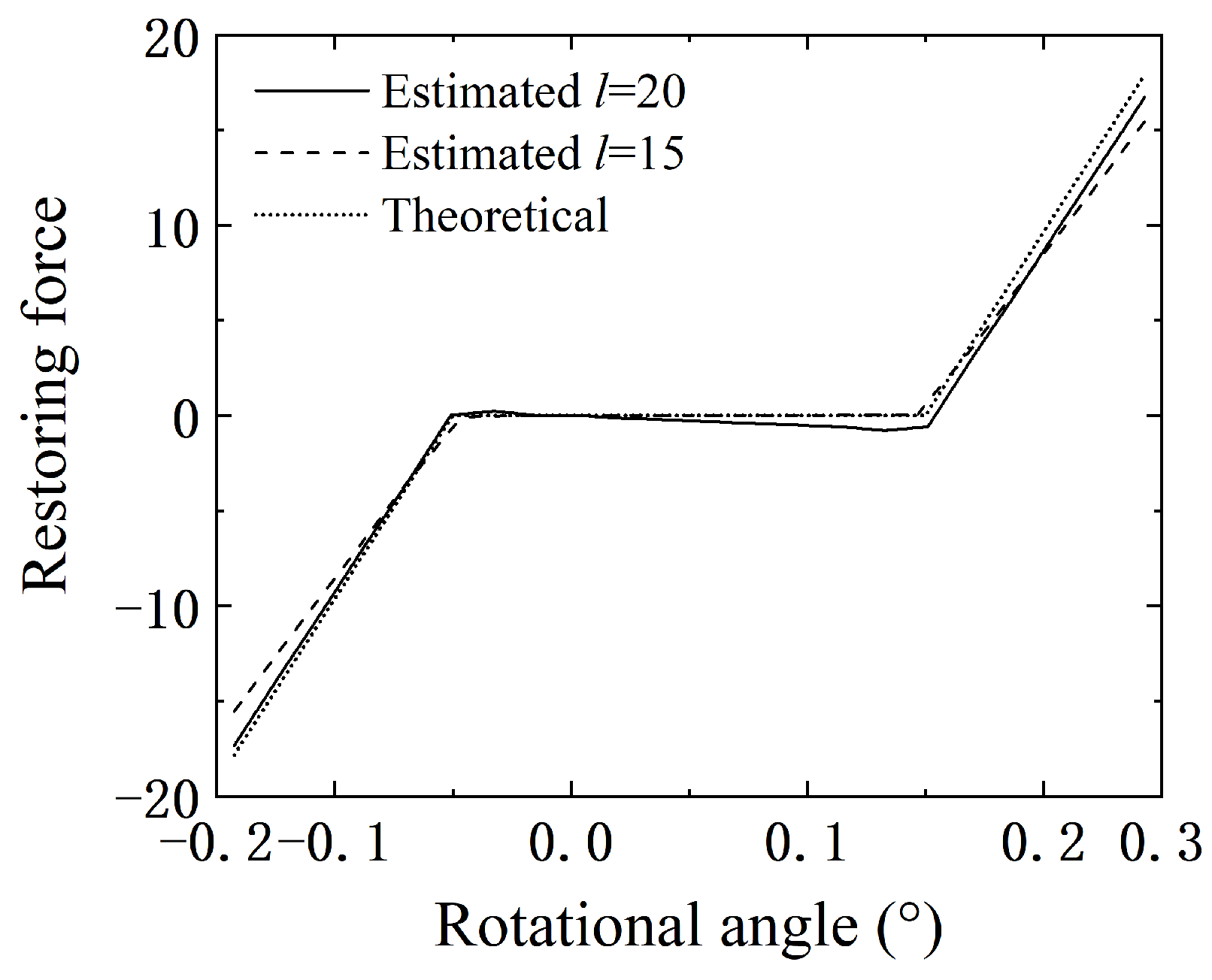
Figure 15.
The identification of offset freeplay using the 2nd displacement range.

Figure 16.
Stabilization diagram of OLS of offset freeplay computed by TNSI method using the estimated FRF(). (Dot: Not stable in frequency; Circle: Stable in frequency; Cross: Stable in frequency and damping).
Figure 16.
Stabilization diagram of OLS of offset freeplay computed by TNSI method using the estimated FRF(). (Dot: Not stable in frequency; Circle: Stable in frequency; Cross: Stable in frequency and damping).

Table 1.
Natural frequencies and damping ratios of the first 2 modes of all movable fin up to 150 Hz.
Table 1.
Natural frequencies and damping ratios of the first 2 modes of all movable fin up to 150 Hz.
| Mode | Natural Frequency (Hz) | Damping Ratio (%) | Description |
|---|---|---|---|
| 1 | 90.6 | 0.72 | Rigid fin bending mode |
| 2 | 102.1 | 0.56 | Rigid fin rotating mode |
Table 2.
The parameters of freeplay.
| Type | Parameters | Value |
|---|---|---|
| Central freeplay | d | |
| Offset freeplay | ||
Table 3.
The natural frequencies identified by TNSI method.
| Mode | Natural Frequency (Hz) | Identified Natural Frequency (Hz) | Errors (%) | |
|---|---|---|---|---|
| FE Model | Central Freeplay | Offset Freeplay | ||
| 1 | 90.6 | 90.8 | 90.8 | 0.22 |
| 2 | 102.1 | 102.5 | 102.5 | 0.39 |
© 2020 by the authors. Licensee MDPI, Basel, Switzerland. This article is an open access article distributed under the terms and conditions of the Creative Commons Attribution (CC BY) license (http://creativecommons.org/licenses/by/4.0/).
Share and Cite
MDPI and ACS Style
Yukai, S.; Chao, Y.; Zhigang, W.; Liuyue, B. Nonlinear System Identification of an All Movable Fin with Rotational Freeplay by Subspace-Based Method. Appl. Sci. 2020, 10, 1205. https://doi.org/10.3390/app10041205
AMA Style
Yukai S, Chao Y, Zhigang W, Liuyue B. Nonlinear System Identification of an All Movable Fin with Rotational Freeplay by Subspace-Based Method. Applied Sciences. 2020; 10(4):1205. https://doi.org/10.3390/app10041205
Chicago/Turabian StyleYukai, Sun, Yang Chao, Wu Zhigang, and Bai Liuyue. 2020. "Nonlinear System Identification of an All Movable Fin with Rotational Freeplay by Subspace-Based Method" Applied Sciences 10, no. 4: 1205. https://doi.org/10.3390/app10041205
Note that from the first issue of 2016, this journal uses article numbers instead of page numbers. See further details here.