Evaluating Slope Deformation of Earth Dams Due to Earthquake Shaking Using MARS and GMDH Techniques

Abstract

Assessing the behavior of earth dams under dynamic loads is one of the most significant problems with the design of such large structures. The purpose of this study is to provide new models for predicting dam dispersion in real earthquake conditions. In the first phase, 103 real cases of deformation in earth dams were collected and analyzed due to earthquakes that occurred over recent years. Using nonlinear and machine learning techniques, i.e., group method of data handling (GMDH) and multivariate adaptive regression splines (MARS), two models for prediction of the slope deformation in earth dams under the various types of earthquakes were applied and developed. The main parameters used in these simulation techniques were earthquake magnitude (Mw), fundamental period ratio (Td/Tp), yield acceleration ratio (ay/amax) as inputs and value of slope deformation (Dave) as output. Finally, in order to check the accuracy of the results of the new models, a comparison was made with the previous relations and models in seismic conditions for the slope deformation in earth dams. The results showed that the MARS model, which is able to provide a mathematical equation, has a better result than the GMDH model. These new models are recommended to be used for future analyses based on their flexible capabilities.

1. Introduction

In seismic loading, the study of dams’ behavior is a necessary and important issue. A wrong study of dams’ behavior in these conditions may result in irreversible damages. The first method to obtain the permanent slope deformation in dams was introduced by Newmark [1] as the sliding block. This method simply calculates changes of slope in the earthquake conditions. Among the primary and basic assumptions of the sliding block method is considering slide mass as a rigid body as well as the greater magnitude of acceleration arising from the earthquake than the yield acceleration that can result in movement of the mass [2,3]. This method was later modified and developed by scholars [4,5]. For example, considering the acceleration of the block response as the input acceleration of the system, Makdisi and Seed [6] evaluated the value of displacement with modification of the block model. Uncertainty of results between real cases and the suggested method has been discussed as well [7]. Moreover, using the numerical methods, such as finite element and finite difference methods, deformations in the earth slopes were obtained [5,8]. In different works, the main parameters of ground motion were used through which the changes of the slope deformation in different conditions in earth dams were studied [9,10]. Hynes-Griffin and Franklin [11] have deformations of dams based on the two features of failure acceleration and maximum acceleration irrespective of the vertical section of acceleration during an earthquake. In general, earthquake issues are very complicated in different subjects [3,12]. Furthermore, other important factors, such as the fundamental period of the dam, non-homogeneity, and settlement characteristics, have different impacts on huge structures, such as an earth dam [13]. Many scholars have referred to the high complication of the precise relations of these factors in the study of deformations in the earth dam during an earthquake and have considered it as an important challenge in the geotechnical area [14,15,16].

In recent years, new methods based on soft computing have been used in different engineering analyses considering the ability to solve complicated problems. These methods, in fields of civil engineering and the geotechnical area, have been applied to different issues, such as the dynamic behavior of earth, deformations of earth, tunneling, and laboratory samples of mines [17,18,19,20,21,22,23,24,25,26,27,28,29,30,31,32,33,34,35,36,37,38,39,40,41,42,43,44,45,46,47,48,49,50,51,52,53,54,55,56,57,58,59,60,61,62,63,64,65,66,67]. There are a few researches concerning the use of soft computing methods in the earth dams’ deformations arising from earthquakes. It shows that a new methodology, based on these methods, for earth dams’ deformations can be developed and implemented. Therefore, in this study, given the above discussions, two new methods of soft computing, i.e., group method of data handling (GMDH) and multivariate adaptive regression splines (MARS), were implemented to evaluate the slope deformations of earth dams. These models were selected to propose a black box model (GMDH) and mathematical formula (MARS) in predicting slope deformation. In addition, these types of intelligent models have unique features for comparison purposes. To this end, the data of different earthquakes were gathered from around the world. Then, the initial analyses were performed on them. Using the initial analyses, the intelligence models predicted the slope deformations. In the end, new models were compared with the old models. The rest of this paper will continue by giving some information about the case study and data collection. After that, the principles of MARS and GMDH models and their implementation in predicting slope deformation will be given in detail. Finally, the most appreciated model will be selected through the use of some well-known performance indices.

2. Case Study of Earth Dam

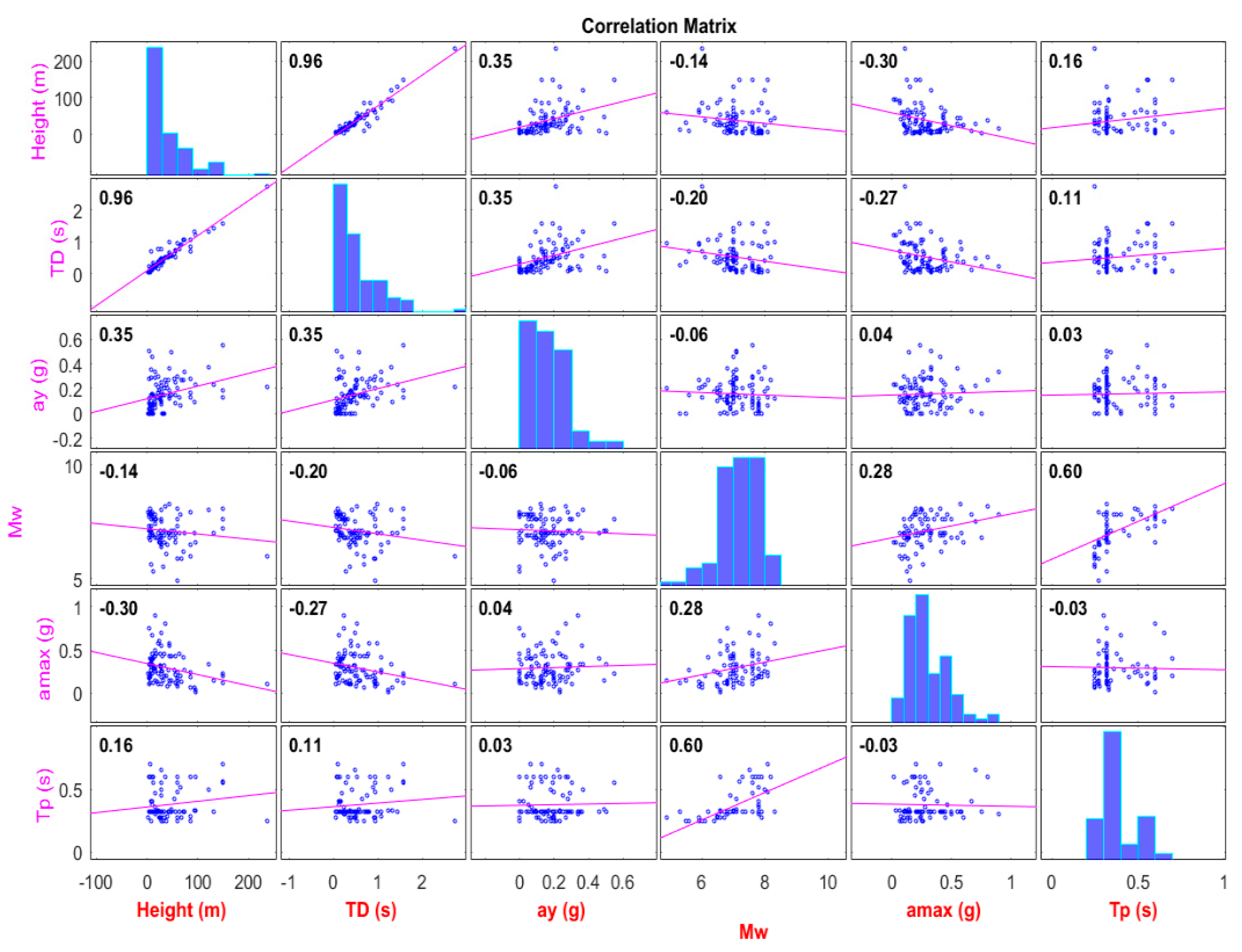
In this study, a dataset of the slope changes of earth dams and embankments that are created during earthquakes was gathered from around the world. This dataset includes a various range of dams, including homogeneous and non-homogeneous earth dams, embankment dams with concrete facing, rockfill dams, and a few natural slopes. Various recorded data of these samples have been presented in studies and reports [68,69,70,71,72,73,74,75]. The gathered parameters include earthquake magnitude (Mw), yield acceleration ratio (ay/amax), fundamental period ratio (Td/Tp), and value of slope deformation (Dave) for the collected results that have been obtained from 103 real cases. Figure 1 shows the different distributions of these data.

The Dave parameter indicates the movement toward the lower section of the earth along the sliding surface that is created by an earthquake. In fact, this value is a point of the vertical and horizontal components of deformations and is calculated in the form of a single vector in the direction of the base of the sliding surface. Using the critical failure arising from the quasi-static analyses, the base inclination angle is derived. Other parameters, such as Mw, amax, and Tp, refer to the earthquake magnitude, the horizontal component of the maximum acceleration of earthquake and predominant earthquake period, respectively, which are introduced as seismic loading features. The two parameters of ay and Td are also called geotechnical features of earth dams and imply the yield acceleration and fundamental period of the earth dam, respectively. The threshold acceleration occurs when a mass is sliding downward, and using the quasi-static analyses, this value is obtained as yield acceleration as in [76]. The ay parameter, in fact, is the same acceleration value that is obtained equal to 1 in the safety coefficient of static analyses. To obtain the parameter of the fundamental period of the earth dam, generally, the reported previous resources are used. Otherwise, it is computed using the relation of Td = 4H/Vs, which has been suggested by several scholars [4]. In this regard, the parameters of H and Vs show the height of the dam and the shear wave velocity in the body of the dam, respectively. In this study, five parameters of Mw, ay/amax, and Td/Tp, which were the key parameters obtained by the review of the previous studies, are used as the input of the intelligent models [3,77].

In the modeling stage, according to the previous studies, 80% of data are used for training systems and 20% for the test stage [78,79,80,81]. The data are selected by random and this process is repeated several times until the final outputs are obtained, ideally containing less error. The parameters are selected the same in both sections. Finally, the models are obtained for the next analyses and compared with the existing models. The statistical information of the used data (5 parameters as input) are presented in

Table 1. Information on the parameters used in this study.

Parameter	Height (m)	TD (s)	Ay (g)	Mw	Amax (g)	Tp (s)	Dave (m)
Min	2.500	0.050	0.000	4.900	0.010	0.250	0.001
Average	40.389	0.555	0.176	7.045	0.293	0.374	0.883
Max	235.000	2.740	0.550	8.300	0.900	0.700	6.546
Type	Input	Input	Input	Input	Input	Input	Output

.

3. Methodology

3.1. Group Method of Data Handling (GMDH)

The GMDH method is a self-organized algorithm and can provide a good solution for problems that have unknown nature. In fact, this method is a branch of artificial neural network that models the behavior of a phenomenon based on the input and output dataset. Dataset is a pair of data that is composed of several input parameters and one corresponding output parameter (Xi,yi) (=1,2, …,M). Quadratic node is a computational function that is defined based on a transfer function in a feed-forward network. In the GMDH method, in order to define coefficients of this function, a regression analysis is used [82]. In a model that is built by the GMDH method, there are some neuron layers, and several data pairs in every layer are linked with each other by a quadratic polynomial. In this way, new neurons are made. Input and output data are linked and correspond with each other based on the same process [17,83].

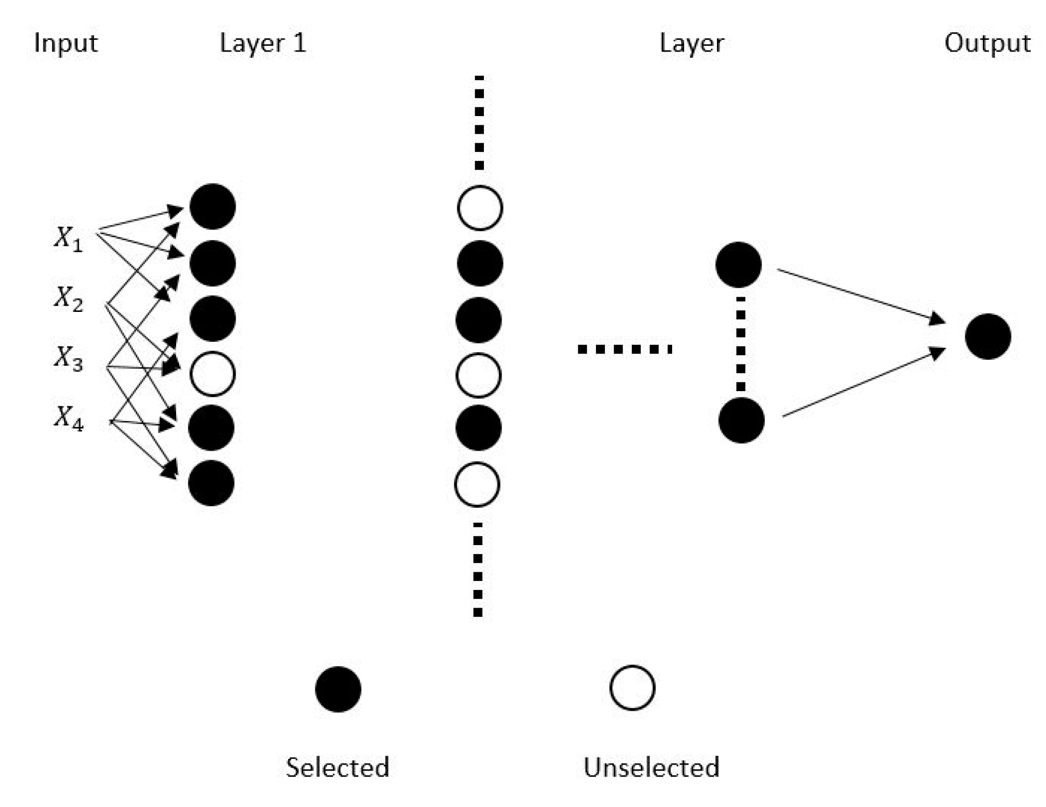
The structure of this process is shown in Figure 2. According to this figure, four parameters are first entered in the first layer, and some functions are defined in this layer. Then, based on this criterion, these functions are selected and transferred to the next layer. The output of the model is also a function that is built in the last layer. The general function of parameters is given in Equation (1).

$$\widehat{y_i}=f\left(X_{i1}, X_{i2}, X_{i3}, \dots X_{in}\right),\left(\mathrm{i}=2,3,\dots \mathrm{M}\right)$$

(1)

Obtaining the parameters in Equation (2) is one of the main steps in this modeling.

$$y=a_0+{\displaystyle \sum }_{i=1}^n{a}_i{x}_i+{\displaystyle \sum }_{i=1}^n{\displaystyle \sum }_{j=1}^n{a}_{ij}{x}_i{x}_i+{\displaystyle \sum }_{i=1}^n{\displaystyle \sum }_{j=1}^n{\displaystyle \sum }_{k=1}^n{a}_{ijk}{x}_i{x}_i{x}_k+\dots$$

(2)

In fact, the above-mentioned parameters are obtained from the solution of a mathematical relation in which the most important parameter among them is the “a” coefficient. In each layer, several functions are defined to obtain the “a” parameter, and this process is repeated until Equation (3) is minimized. If needed, for more information about research in this area, see [39].

$$E=\frac{{{\displaystyle \sum }}_i^M=1{\left(y_i-y\left(x_i,x_j\right)\right)}^2}{M}$$

(3)

In each layer, with the help of neurons, the computational functions are defined. The selection pressure criterion is defined in several layers in order to select parameters. Based on the mentioned criterion, if the built function has the desired conditions, it is transferred to the next layer or otherwise deleted. Equation (4) shows the mentioned criterion in the form of a mathematical relation. The range of change of this parameter is [0, 1]. In order to select a function that has the minimum error, the value of α is considered to be 1. On the other hand, if the value of α is considered close to zero, more data are transferred to the next layer.

$$e_c=\mathsf{\alpha }\times RMS{E}_{min}+\left(1-\alpha \right)\times RMS{E}_{max}$$

(4)

Figure 3 shows the modeling process in which all cases that are applied to run the GMDH model are considered. In order to evaluate the model results, two indices of the correlation coefficient and root mean square error (R², RSME) were used.

$$R^2=\left(1-\frac{{{\displaystyle \sum }}_{q=1}^{Nu{m}_{todo}}{\left(Y_q-{\widehat{Y}}_q\right)}^2}{{{\displaystyle \sum }}_{q=1}^{Nu{m}_{todo}}{\left(Y_q-{\overline{Y}}_q\right)}^2}\right)$$

(5)

3.2. Multivariate Adaptive Regression Splines (MARS)

MARS is a non-parametric regression method, developed by Friedman [84]. The model takes the form of development in the production of basis spline functions, where a number of basic functions (BFs) and the parameters related to each function (product degree and knot location) are automatically determined by the data. The main difference between MARS and non-adaptive spline is that in the former, knots are not pre-determined; they are placed at the best possible locations by a search method. In the case of having only one knot, any possible location in the definition span of an explanatory variable, $Z=\left[ab\right]\in R$ (where a and b are MARS nodes, which should be designed during model development) is considered, and after fitting, a model with a minimum value of sum square error (SSE) is selected. In the case of having two knots, finding the best location for this pair of points requires more calculations and, a fortiori, to have n knots, finding the best n number set of points is very difficult and complicated. The required number of knots is also not known. In the MARS method, the number and location of the required knots are determined through a step-by-step forward-backward process.

BFs are a set of functions that can demonstrate information existing in one or more variables (Figure 4). MARS uses the expansion of piecewise linear basis functions in the forms of (x − t)+ and (t − x)+, also called hinge functions or hockey sticks, and “+” means the positive section, thus [85]:

$${(t-x)}_{+}=\{\begin{array}{ll}t-x,& \mathrm{if}\mathrm{x}<\mathrm{t},\\ 0,& \mathrm{otherwise}.\end{array},{(x-t)}_{+}=\{\begin{array}{ll}x-t,& \mathrm{if}\mathrm{x}>\mathrm{t},\\ 0,& \mathrm{otherwise}.\end{array}$$

(6)

where x is the variable, and t is the knot constant. The MARS algorithm makes a regression model function according to Figure 4.

$$f(x)={\displaystyle \sum _{i=0}^{M-1}{\beta }_i{h}_i(x)}$$

(7)

where x = [x₁,x₂,..,x_p]T is a vector of explanatory variables and p is the dimension of input variables, β_ih_i(x) represents terms of the model that are automatically selected by the algorithm, h_i(x) signifies the basis functions in MARS, and M is the number of terms in the model. Furthermore, assume that (x_i, y_i), i = 1,..,n forms the observations set. Finally, there are two modes for Equation (7). If the defined functions are considered as the basis functions h_i(x), the predictive model obtained by Equation (7) is called non-adaptive; on the other hand, if these functions are determined by modeling data set (x_i, y_i), it is called adaptive, like the MARS model.

3.2.1. Forward Phase

Forward selection phase is the same as the case in piecewise linear regression; it just differs in the point that it uses the A set functions (including all of the functions of h_1i, h_2i, i = 1,…,n and product of two or more of these functions) instead of explanatory variables. This phase is started by considering y-intercept term a0 (average of response values), then the basis functions are repeatedly added as pairs, and corresponding β coefficients are estimated in Equation (7) by minimizing the SSE. In each step of this phase, MARS finds a pair of basis functions that have the highest reduction in SSE. At the end of the phase, a large model is formed with a large number of terms having unsuitable performance in response to the prediction for new data. In other words, this model causes data over-fitting; therefore, it will need a backward deletion phase to achieve the best number of terms [86].

3.2.2. Backward Phase

In order to make a model with higher generalization capacity, the backward phase prunes the model. The backward deletion phase starts its work with the largest model (based on number of MARS equations) obtained at the end of the forward model and, in each step, deletes the least important basis function (according to general cross validation, GCV criterion) that has a minimum share in residual sum of squares. By deletion of each basis function, a new model is estimated that may be a nominee for the final model. The forward phase adds terms in pairs. However, in the backward phase, distinctively, one side of the pair is deleted; therefore, there will be no pair in the final model. The performance of the new model is assessed considering the GCV criterion. The backward phase deletes terms one by one; indeed, it deletes the least effective term in each step to reach the best sub-model. MARS selects the optimal model with the minimum GCV value. The raw residual sum of squares (RSS) of the training set is unsuitable for model comparison because when the MARS terms are deleted, RSS normally increases. In other words, if RSS is used for model comparison, the backward phase will always choose the largest model (based on the number of MARS equations). Assume that GCVk belongs to the k-th model in the deletion phase and is defined by the following relation [84]:

$$GC{V}_K=\frac{1}{n}{\displaystyle \sum _{i=1}^n(y_i-}{{\displaystyle f}}_k(x_i){)}^2/{(1-C(k)/n)}^2$$

(8)

where f_k is the estimated model in the k-th step of the backward deletion phase, and C(k) is the number of effective parameters in the model that is equal to the number of the model’s terms plus the number of parameters used for selection of the best knot locations, in other words:

C(k) = the number of the model’s terms (BF) at the k-th step + λ (the number of the model’s terms (BF) at the k-th step -1)/2, where λ is a smoothing parameter (penalty per knot (GCV)) and is practically selected between 2 and 4. Additionally, BF is basic function. It should be noted that the clause “(the number of the model’s terms (BF) at the k-th step -1)/2” indicates the number of hinged functions’ knots h existing in the model [84].

4. Results and Discussion

4.1. GMDH Simulation

In this section, the GMDH model was implemented for evaluating the slope deformation of earth dams. Of the data sets collected in this study, about 80% of the data were used to design and train models randomly. Different models were designed to obtain the least error model. Finally, the remaining data (20% of the total data) were used to evaluate the power of the models [87,88,89]. The code for the GMDH model was implemented in MATLAB software. According to the description given in the previous section, the GMDH model is designed by various components that control system performance. In order to design the best model, the impacts of each were evaluated under different conditions to obtain the best model to predict the slope deformation of earth dams.

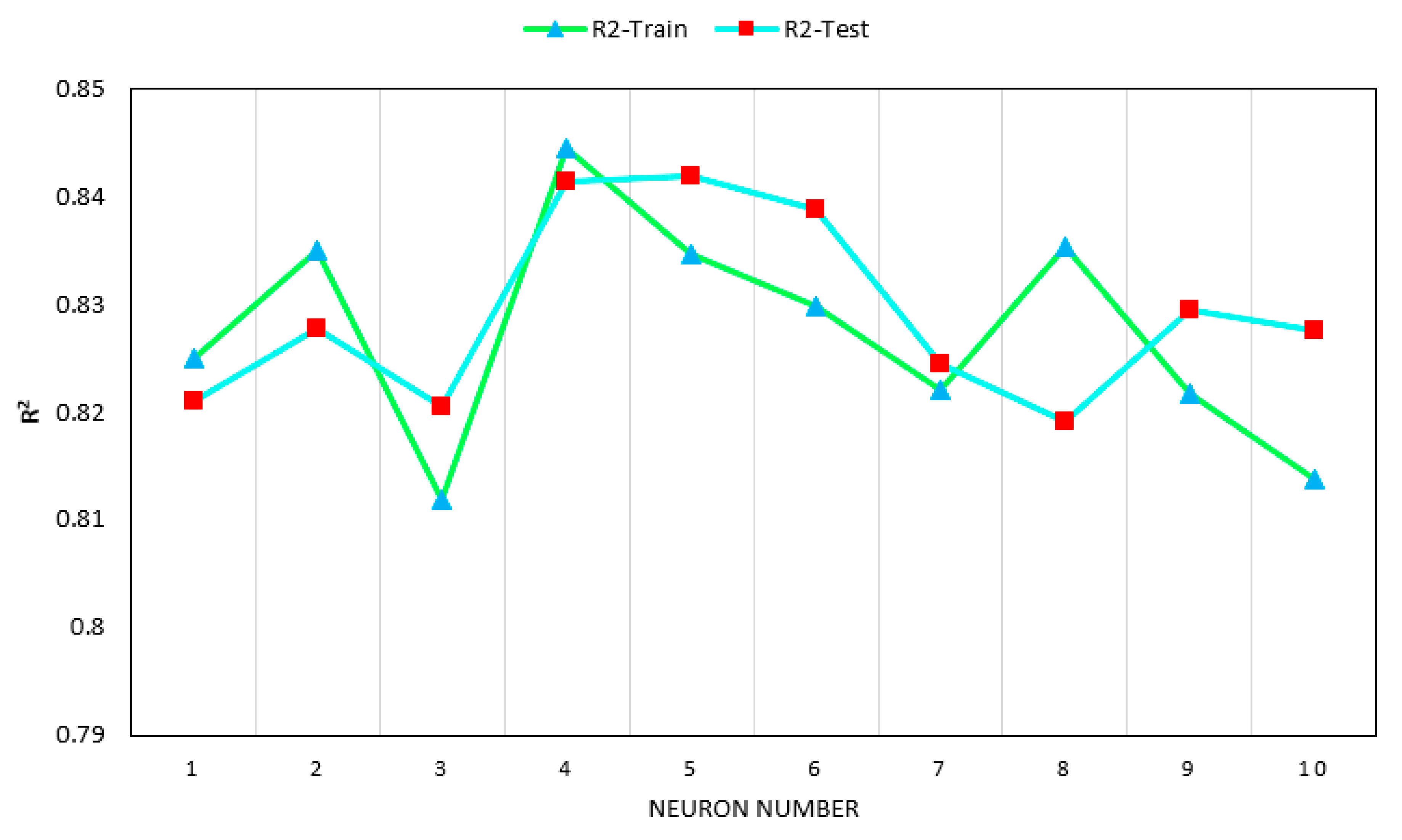
One of the most important parts of intelligent models is the number of neurons used in the system and their layers. In the GMDH model, this parameter is also effective. According to the recommendation of previous research and initial analysis for these data, the number of neurons in different layers of GMDH ranged from 1 to 10. The number of neurons defined in this model is, in fact, the maximum number of neurons that each layer used according to the solution conditions. In other words, it is possible for each layer to use less than the maximum number of neurons to solve the problem. For this reason, the analysis of this study is presented in Figure 5. As can be seen, the results are presented for both training and testing sections to obtain the performance of each model. For the data of this study, the best condition is obtained with four neurons. As can be seen, the proximity of the training and testing results shows that the simulation is presented with acceptable accuracy. In addition, models with higher neurons show less accuracy than this model; thus, it can be indicated that the model with four neurons is the optimal one.

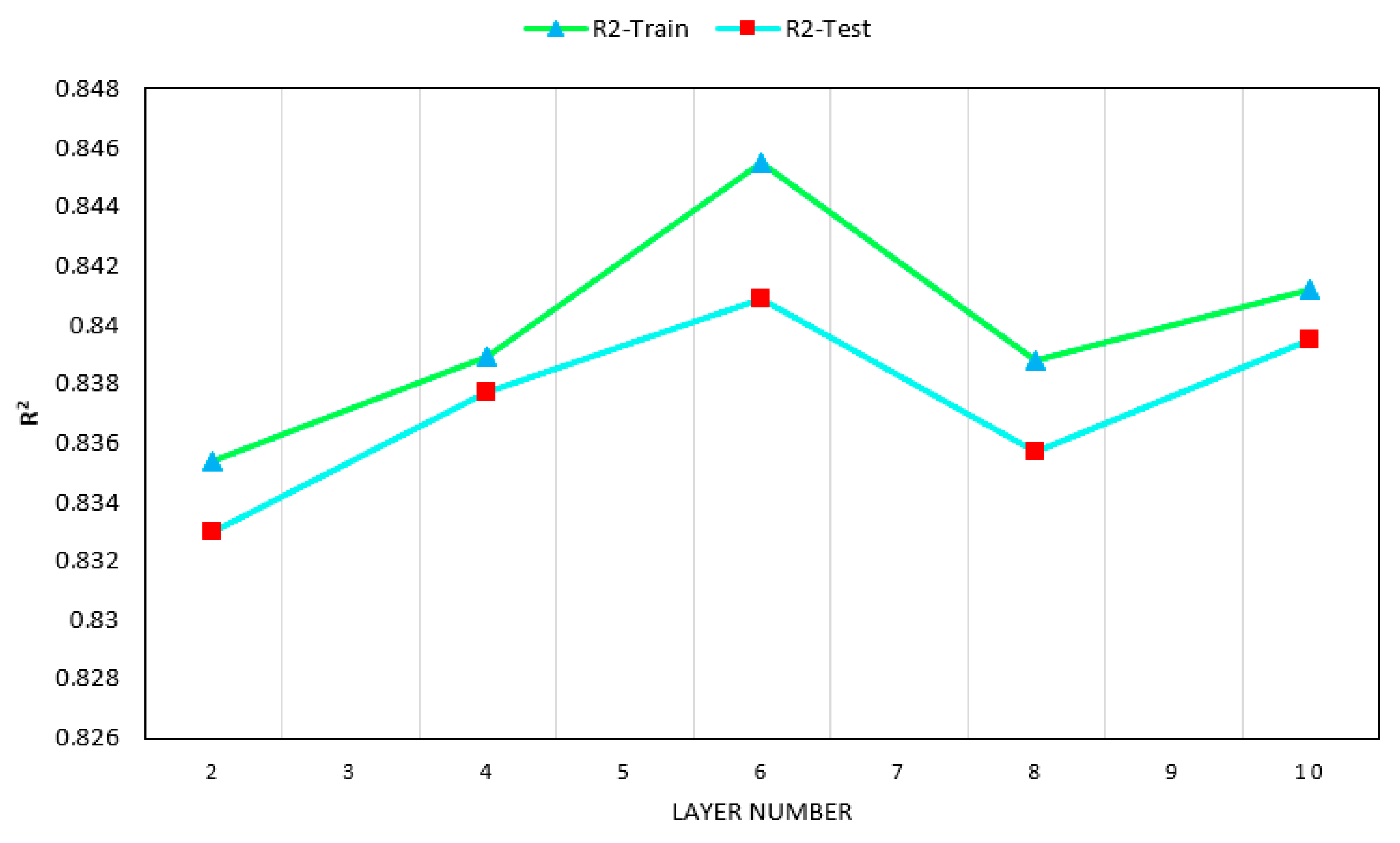
Based on the analysis of the previous step, in this step, the effect of the number of layers applied in the GMDH model is investigated. The difference between the number of layers of this model compared to other intelligent models is that the number of layers can be more than one depending on the problem. However, most artificial intelligence works have recommended a layer for solving most linear and nonlinear problems. The GMDH model, with more layers, can also provide convergence conditions to specific conditions. Hence, five layers (2,4,6,8,10) were evaluated. The results for the different sections are presented in Figure 6. As can be seen, the effect of the number of layers on the results is different. The best performance is the six-layer model, of which its results can be introduced as an optimized model.

Finally, the third important factor that influences the GMDH method is investigated by parametric analysis. Selection pressure is a criterion that allows the data of each layer to know what number of the previous section data can be used for continuing analysis. This criterion actually selects the number of data that best fits each step and sets it as the next layer input, repeating it until the final steps, so that the system achieves the lowest error and highest accuracy. In this case, one should choose the model that offers the best runtime and accuracy. The results of this study are shown in Figure 7. As can be shown, the best value for selection pressure is 40%. This also indicates the high accuracy of the model that was able to predict the data well. Finally, the final model for predicting the slope deformation of earth dams using the GMDH method is introduced at this stage. The best model was able to provide a system with R² = 0.8489 and 0.8458 accuracy for the training and testing sections, respectively. In the next section, the new MARS model is implemented for this problem.

4.2. MARS Modeling

Likewise, the data were divided into two sets for training and testing with percentages of 80% and 20%, respectively. As mentioned before, MARS is sensitive to its initial parameters. Thus, there is a need for determining the most effective parameters on the MARS model with their suitable ranges. MARS effective parameters with their suitable range/value are shown in

Table 2. Multivariate adaptive regression splines (MARS) effective parameters with their range/value used in the study.

Parameter	Range/Value
Self-interactions	No
Prune	Yes
Max Functions	5–20
Generalized cross-validation penalty per knot	0,1,2
Max interactions	2–4
Threshold	1.00 × 10−5

. It should be noted that the MARS model was constructed in a MATLAB environment to estimate the slope deformation of earth dams.

Examining different conditions for designing models can give various results. Using these results, the main objective of this research can be achieved by presenting a new model for assessing slope deformation of earth dams due to earthquake shaking. Several MARS models based on ranges mentioned in

Table 3. Proposed MARS model based on the piecewise-linear method.

Basis Function	Values/Expression
BF1 =	max(0, x3 − 0.04)
BF2 =	max(0, x3 − 0.1)
BF3 =	BF2 * max(0, x6 − 0.6)
BF4 =	BF2 * max(0,0.6 − x6)
BF5 =	max(0,7.8 − x4)
BF6 =	max(0, x4 − 7.3)
BF7 =	max(0,7.3 − x4)
BF8 =	BF6 * max(0, x1 − 6)
BF9 =	BF6 * max(0,6 − x1)
BF10 =	BF8 * max(0, x3 − 0.12)
BF11 =	BF8 * max(0,0.12 − x3)
BF12 =	BF11 * max(0, x2 − 0.24)
BF13 =	BF11 * max(0,0.24 − x2)
BF14 =	max(0,0.1 − x3) * max(0,12 − x1)
BF15 =	BF14 * max(0, x2 − 0.09)
BF16 =	BF14 * max(0,0.09 − x2)
BF17 =	BF8 * max(0, x2 − 0.25)
BF18 =	BF8 * max(0, x2 − 0.42)
BF19 =	BF8 * max(0,0.42 − x2)
BF20 =	BF19 * max(0, x5 − 0.5)
BF21 =	BF19 * max(0,0.5 − x5)
BF22 =	max(0, x4 − 8)

were constructed to predict slope deformation of earth dams. Then, the best MARS model was selected according to the obtained prediction performance. As mentioned earlier, MARS is able to propose a relationship between model inputs and model output. In the following, two different methods of MARS techniques are used to evaluate the slope deformation of earth dams.

4.2.1. Piecewise-Linear Method

In the first technique, linear nodes are used to create data prediction conditions. Each variable (X1 to X6) is considered under different conditions and creates states to evaluate the slope deformation of earth dams. All the states between these variables for the prediction are given in Figure 8. As can be seen, these scenarios are designed for a variety of linear conditions and ultimately provide a MARS model to predict the slope deformation of earth dams. The results of this model are presented in

Table 4. Results of slope deformation of earth dam predicted by the MARS model based on the piecewise-linear method.

Training		Testing
MAE	0.3057	MAE	0.2767
MSE	0.2571	MSE	0.2165
RMSE	0.5070	RMSE	0.4653
RRMSE	0.3456	RRMSE	0.3072
R2	0.8905	R2	0.8956

. Finally, the structure of the model is presented using Table 4 and Equation (8).

y = 5 + 4.4 × BF1 − 10 × BF2 + 9.4 × 10² × BF3 + 17 × BF4 − 9.6 × BF5 − 6.6 × BF6 + 9.6 × BF7 + 1.8 × BF8 − 0.86 × BF9 + 0.13 × BF10 + 21 × BF11 − 4.1 × 10² × BF12 –10² × BF13 + 14 × BF14 − 79 × BF15 − 3.1 × 10² × BF16 − 11 × BF17 + 11 × BF18 − 6.5 × BF19 − 9.1 × BF20 − 10 × BF21 + 9.1 × BF22

(9)

This relationship can be a good solution for issues that need to be more realistic. This formula is one of the advantages of the MARS method that can be used in various fields of geotechnical and civil engineering. Using this relationship, the slope deformation of earth dams can be determined with an accuracy of R² = 0.8905 and 0.8956 for two sections of training and testing the MARS model based on the piecewise-linear technique.

4.2.2. Piecewise-Nonlinear Method

In the second method, instead of using linear nodes, nonlinear conditions are considered. As in the first method, different states of influence of the input parameters on the output are obtained, and finally, using them, the MARS model is created. Figure 9 illustrates the results of nonlinear states. The accuracy of this new model is given in

Table 5. Results of slope deformation of earth dam predicted by the MARS model based on the piecewise-cubic method.

Training		Testing
MAE	0.5343	MAE	0.5347
MSE	0.5259	MSE	0.5659
RMSE	0.7252	RMSE	0.7523
RRMSE	0.4944	RRMSE	0.4968
R2	0.7556	R2	0.7532

. As can be seen from this table, the results of the first method were better in predicting the slope deformation of earth dams. The results of the piecewise-cubic method are presented in

Table 6. Proposed MARS model based on the piecewise-cubic method.

Basis Function	Values/Expression
BF1 =	C(x3| + 1,0.02,0.04,0.07)
BF2 =	C(x3| + 1,0.07,0.1,0.11)
BF3 =	BF2 * C(x6| + 1,0.42,0.6,0.65)
BF4 =	BF2 * C(x6| − 1,0.42,0.6,0.65)
BF5 =	C(x4| − 1,7.5,7.8,7.9)
BF6 =	C(x4| + 1,6.1,7.3,7.5)
BF7 =	C(x4| − 1,6.1,7.3,7.5)
BF8 =	BF6 * C(x1| + 1,4.3,6,8.8)
BF9 =	BF6 * C(x1| − 1,4.3,6,8.8)
BF10 =	BF8 * C(x3| + 1,0.11,0.12,0.34)
BF11 =	BF8 * C(x3| − 1,0.11,0.12,0.34)
BF12 =	BF11 * C(x2| + 1,0.16,0.24,0.25)
BF13 =	BF11 * C(x2| − 1,0.16,0.24,0.25)
BF14 =	C(x3| − 1,0.07,0.1,0.11) * C(x1| − 1,8.8,12,1.2e + 02)
BF15 =	BF14 * C(x2| + 1,0.07,0.09,0.16)
BF16 =	BF14 * C(x2| − 1,0.07,0.09,0.16)
BF17 =	BF8 * C(x2| + 1,0.25,0.25,0.33)
BF18 =	BF8 * C(x2| + 1,0.33,0.42,1.6)
BF19 =	BF8 * C(x2| − 1,0.33,0.42,1.6)
BF20 =	BF19 * C(x5| + 1,0.26,0.5,0.7)
BF21 =	BF19 * C(x5| − 1,0.26,0.5,0.7)
BF22 =	C(x4| + 1,7.9,8,8.2)

below. These functions eventually provide a relationship to predict the slope deformation of earth dams in Equation (10).

y = 4.8 − 22 × BF1 + 11 × BF2 + 8.3 × 10² × BF3 + 38 × BF4 − 5.5 × BF5 + 1.3 × BF6 + 5.1 × BF7 + 1.4 × BF8 − 2.3 × BF9 + 0.26 × BF10 + 4.9 × BF11 − 4.4 × BF12 − 14 × BF13 + 1.6 × BF14 − 2.5 × BF15 − 50 × BF16 − 8.9 × BF17 + 9 × BF18 − 8.5 × BF19 − 1.2 × BF20 − 2.2 × BF21 + 1.2 × BF22

(10)

This relationship can be a good solution for issues that need to be more realistic. This formula is one of the advantages of the MARS method that can be used in various fields of geotechnical and civil engineering.

Finally, the best model obtained for the slope deformation of earth dams distance prediction is presented in Table 6. As can be seen, its performance is better than the GMDH and second method of MARS. As a result, the first method of the MARS model (piecewise-linear) can be successfully applied to making such predictions in a reasonably accurate way.

5. Evaluation of the Performance of MARS Technique and the Old Models

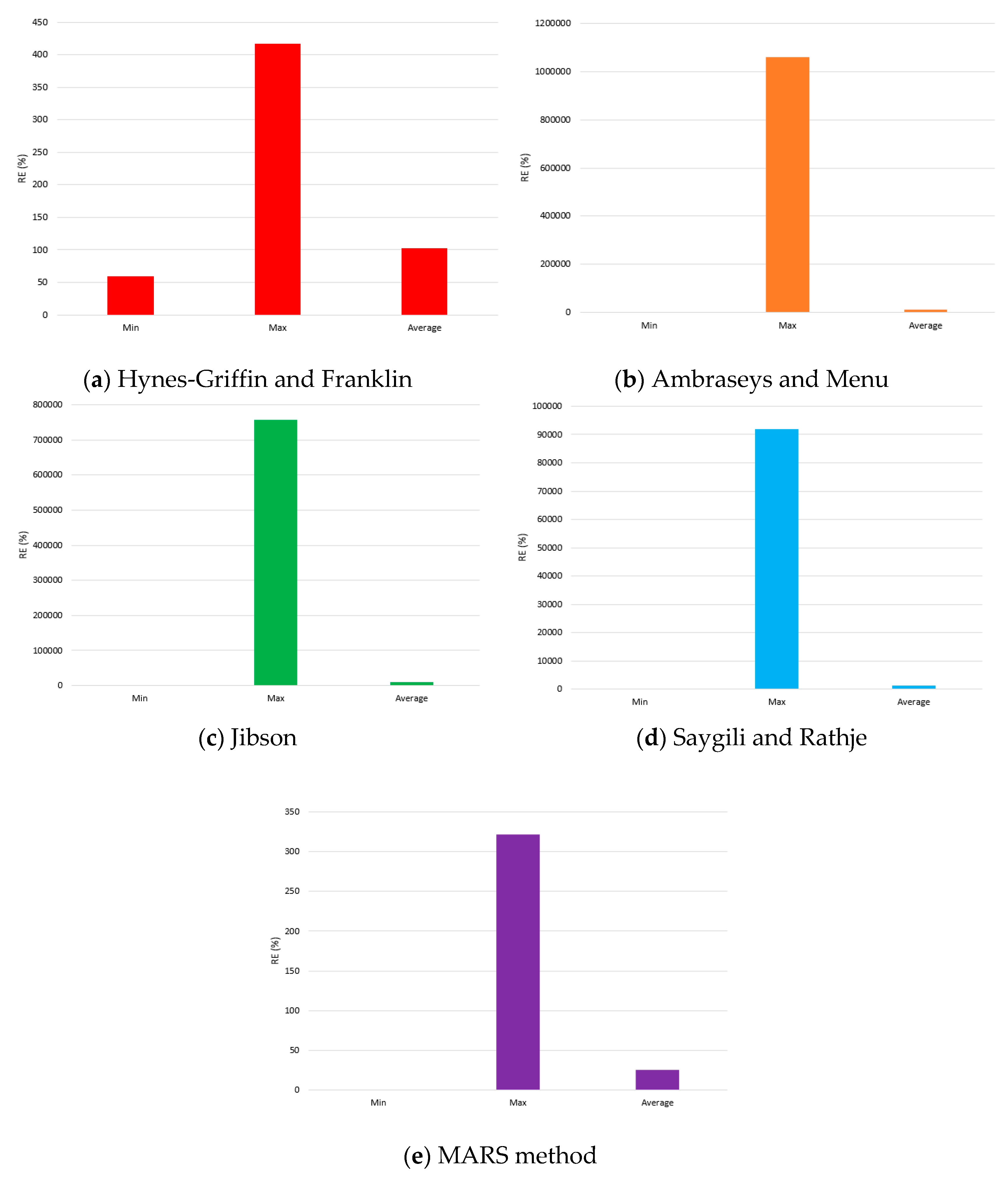
In this section, a comparison has been made between the models developed in this study and the old models developed by previous scholars [6,11,77,90,91].

Table 7. The models developed for determining the value of slope deformation (Dave).

Models	Equations	Limitation
Hynes-Griffin and Franklin	$\begin{array}{ll}\log (D_{(cm)})& =-0.287-2.854(\frac{a_y}{a_{\max }})-1.733{(\frac{a_y}{a_{\max }})}^2\\ & -0.702{(\frac{a_y}{a_{\max }})}^3-0.116{(\frac{a_y}{a_{\max }})}^4\end{array}$	$\begin{array}{l}0.01\le a_y/a_{\max }\le 0.6\\ M_w\le 8\end{array}$
Ambraseys and Menu	$\log (D_{(m)})=0.9+\log [{(1-\frac{a_y}{a_{\max }})}^{2.53}\times {(\frac{a_y}{a_{\max }})}^{-1.09}]$	$\begin{array}{l}0.05\le a_y/a_{\max }\le 0.95\\ 6.6\le M_w\le 7.2\end{array}$
Jibson	$\begin{array}{ll}\log (D_{(cm)})& =-2.710+\log [{(1-\frac{a_y}{a_{\max }})}^{2.335}\times {(\frac{a_y}{a_{\max }})}^{-1.478}]\\ & +0.424M_w\end{array}$	$\begin{array}{l}0.05\le a_y\le 0.4g\\ a_y/a_{\max }\le 1\\ 5.3\le M_w\le 7.6\end{array}$
Saygili and Rathje	$\begin{array}{ll}\log (D_{(cm)})& =5.52+0.72\ln (a_{\max })-4.43(\frac{a_y}{a_{\max }})\\ & -20.93(\frac{a_y}{a_{\max }})+42.61{(\frac{a_y}{a_{\max }})}^3-28.74{(\frac{a_y}{a_{\max }})}^4\end{array}$	$\begin{array}{l}0.05\le a_y\le 0.3g\\ a_{\max }\le 1g\\ 0.05\le a_y/a_{\max }\le 1\\ 4.5\le M_w\le 7.9\end{array}$

shows the previous models with their unique characteristics that have been extracted and presented for the earth slopes in the effects of an earthquake.

These relations are based on the Newmark block model. For comparison, the relative error (RE) of all the models was obtained using the following relation:

$$RE=\frac{D_{ave-p}-D_{ave-m}}{D_{ave-m}}\times 100$$

(11)

where D_ave-p and D_ave-m are the mean deformations predicted by different models (piecewise-linear method of MARS model and the existing relationships) and the real deformations arising from earthquakes. Results of this comparison have been presented in Figure 10. As it is observed in this figure, the newly developed model provides a more appropriate performance than the other models. Compared to the conventional old models, using the new methods can increase the precision of calculations and designs. One of the major reasons for the high accuracy of the artificial intelligence methods is considering the various complications of the earth structures affected by earthquakes. These models are quicker in calculations and can be a better substitution for the previous models. Finally, the new models can be a positive step in order to reduce uncertainty in the geotechnical problems and particularly the slope deformations of the earth dams.

6. Conclusions

In designing the security of the earth dams, it is necessary to evaluate the slopes in the effect of earthquakes accurately. Therefore, measurement and prediction of this issue in the designs are considered as an important prerequisite. In this study, an attempt was made to predict the value of the slope deformations in the earth dams. To the end, through gathering a set of data from the recorded changes in the real samples, including the parameters of earthquake magnitude (Mw), maximum horizontal earthquake acceleration (amax), yield acceleration of earth dam slope (ay), predominant earthquake period (TP), and fundamental period of earth dam (Td), the results and models were evaluated and analyzed. These parameters were selected as important and effective parameters and introduced as the input to the intelligent models. In this study, the two models of GMDH and MARS were developed and implemented to evaluate the slope deformations in the earth dams created in the effect of an earthquake. These models were evaluated by different examinations, and the effective parameters of each one were identified and evaluated. In the end, a comparison was made between the best models of GMDH and MARS to select the chosen model. The new MARS model could predict the values of Dave with higher performance. The accuracy of the suggested model was obtained R² = 0.8905 and R² = 0.8956 for the test and training sections, respectively. The performance of this model shows the acceptable precision for predictions. After this section, the impact of different parameters on the output was obtained using the sensitivity analysis. Mw and ay were determined as the most effective and the least effective parameters in the prediction models. In the end, a comparison was made between the models developed in this study and the old models. These results show that the present model can predict the value of Dave in the earth dams arising from earthquakes with higher precision.

References

- Newmark, N.M. Effects of earthquakes on dams and embankments. Geotechnique 1965, 15, 139–160. [Google Scholar] [CrossRef] [Green Version]
- Meehan, C.L.; Vahedifard, F. Evaluation of simplified methods for predicting earthquake-induced slope displacements in earth dams and embankments. Eng. Geol. 2013, 152, 180–193. [Google Scholar] [CrossRef]
- Jafarian, Y.; Lashgari, A. Simplified procedure for coupled seismic sliding movement of slopes using displacement-based critical acceleration. Int. J. Geomech. 2016, 16, 4015101. [Google Scholar] [CrossRef]
- Rathje, E.M.; Bray, J.D. Nonlinear coupled seismic sliding analysis of earth structures. J. Geotech. Geoenviron. Eng. 2000, 126, 1002–1014. [Google Scholar] [CrossRef]
- Kramer, S.L.; Smith, M.W. Modified Newmark model for seismic displacements of compliant slopes. J. Geotech. Geoenviron. Eng. 1997, 123, 635–644. [Google Scholar] [CrossRef]
- Makdisi, F.I.; Seed, H.B. Simplified procedure for estimating dam and embankment earthquake-induced deformations. J. Geotech. Geoenviron. Eng. 1978, 104, 849–861. [Google Scholar]
- Strenk, P.M.; Wartman, J. Uncertainty in seismic slope deformation model predictions. Eng. Geol. 2011, 122, 61–72. [Google Scholar] [CrossRef]
- Prevost, J.H.; Abdel-Ghaffar, A.M.; Lacy, S.J. Nonlinear dynamic analyses of an earth dam. J. Geotech. Eng. 1985, 111, 882–897. [Google Scholar] [CrossRef]
- Sarma, S.K. Seismic stability of earth dams and embankments. Geotechnique 1975, 25, 743–761. [Google Scholar] [CrossRef]
- Yegian, M.K.; Marciano, E.A.; Ghahraman, V.G. Earthquake-induced permanent deformations: Probabilistic approach. J. Geotech. Eng. 1991, 117, 35–50. [Google Scholar] [CrossRef]
- Hynes-Griffin, M.E.; Franklin, A.G. Rationalizing the Seismic Coefficient Method; The U.S. Army Corps of Engineers Waterways Experiment Station: Vicksburg, MS, USA, 1984. [Google Scholar]
- Ishihara, K. Soil Behaviour in Earthquake Geotechnics; Oxford University Press: Oxford, UK, 1996. [Google Scholar]
- Rampello, S.; Cascone, E.; Grosso, N. Evaluation of the seismic response of a homogeneous earth dam. Soil Dyn. Earthq. Eng. 2009, 29, 782–798. [Google Scholar] [CrossRef]
- Siyahi, B.; Arslan, H. Earthquake induced deformation of earth dams. Bull. Eng. Geol. Environ. 2008, 67, 397–403. [Google Scholar] [CrossRef]
- Bray, J.D.; Travasarou, T. Simplified procedure for estimating earthquake-induced deviatoric slope displacements. J. Geotech. Geoenviron. Eng. 2007, 133, 381–392. [Google Scholar] [CrossRef]
- Cavallaro, A.; Ferraro, A.; Grasso, S.; Maugeri, M. Site response analysis of the Monte Po Hill in the City of Catania. Am. Ins. Phys. 2008, 1020, 240–251. [Google Scholar]
- Koopialipoor, M.; Nikouei, S.S.; Marto, A.; Fahimifar, A.; Armaghani, D.J.; Mohamad, E.T. Predicting tunnel boring machine performance through a new model based on the group method of data handling. Bull. Eng. Geol. Environ. 2018, 78, 3799–3813. [Google Scholar] [CrossRef]
- Liao, X.; Khandelwal, M.; Yang, H.; Koopialipoor, M.; Murlidhar, B.R. Effects of a proper feature selection on prediction and optimization of drilling rate using intelligent techniques. Eng. Comput. 2019. [Google Scholar] [CrossRef]
- Koopialipoor, M.; Ghaleini, E.N.; Haghighi, M.; Kanagarajan, S.; Maarefvand, P.; Mohamad, E.T. Overbreak prediction and optimization in tunnel using neural network and bee colony techniques. Eng. Comput. 2018, 35, 1191–1202. [Google Scholar] [CrossRef]
- Koopialipoor, M.; Tootoonchi, H.; Jahed Armaghani, D.; Tonnizam Mohamad, E.; Hedayat, A. Application of deep neural networks in predicting the penetration rate of tunnel boring machines. Bull. Eng. Geol. Environ. 2019, 78, 6347–6360. [Google Scholar] [CrossRef]
- Gordan, B.; Koopialipoor, M.; Clementking, A.; Tootoonchi, H.; Mohamad, E.T. Estimating and optimizing safety factors of retaining wall through neural network and bee colony techniques. Eng. Comput. 2018, 35, 945–954. [Google Scholar] [CrossRef]
- Zhou, J.; Aghili, N.; Ghaleini, E.N.; Bui, D.T.; Tahir, M.M.; Koopialipoor, M. A Monte Carlo simulation approach for effective assessment of flyrock based on intelligent system of neural network. Eng. Comput. 2019. [Google Scholar] [CrossRef]
- Liu, B.; Yang, H.; Karekal, S. Effect of Water Content on Argillization of Mudstone During the Tunnelling process. Rock Mech. Rock Eng. 2019. [Google Scholar] [CrossRef]
- Koopialipoor, M.; Murlidhar, B.R.; Hedayat, A.; Armaghani, D.J.; Gordan, B.; Mohamad, E.T. The use of new intelligent techniques in designing retaining walls. Eng. Comput. 2019, 36, 283–294. [Google Scholar] [CrossRef]
- Yang, H.; Liu, J.; Liu, B. Investigation on the cracking character of jointed rock mass beneath TBM disc cutter. Rock Mech. Rock Eng. 2018, 51, 1263–1277. [Google Scholar] [CrossRef]
- Yang, H.Q.; Li, Z.; Jie, T.Q.; Zhang, Z.Q. Effects of joints on the cutting behavior of disc cutter running on the jointed rock mass. Tunn. Undergr. Space Technol. 2018, 81, 112–120. [Google Scholar] [CrossRef]
- Yang, H.Q.; Xing, S.G.; Wang, Q.; Li, Z. Model test on the entrainment phenomenon and energy conversion mechanism of flow-like landslides. Eng. Geol. 2018, 239, 119–125. [Google Scholar] [CrossRef]
- Sarir, P.; Chen, J.; Asteris, P.G.; Armaghani, D.J.; Tahir, M.M. Developing GEP tree-based, neuro-swarm, and whale optimization models for evaluation of bearing capacity of concrete-filled steel tube columns. Eng. Comput. 2019. [Google Scholar] [CrossRef]
- Huang, L.; Asteris, P.G.; Koopialipoor, M.; Armaghani, D.J.; Tahir, M.M. Invasive Weed Optimization Technique-Based ANN to the Prediction of Rock Tensile Strength. Appl. Sci. 2019, 9, 5372. [Google Scholar] [CrossRef] [Green Version]
- Chen, H.; Asteris, P.G.; Jahed Armaghani, D.; Gordan, B.; Pham, B.T. Assessing Dynamic Conditions of the Retaining Wall: Developing Two Hybrid Intelligent Models. Appl. Sci. 2019, 9, 1042. [Google Scholar] [CrossRef] [Green Version]
- Armaghani, D.J.; Hatzigeorgiou, G.D.; Karamani, C.; Skentou, A.; Zoumpoulaki, I.; Asteris, P.G. Soft computing-based techniques for concrete beams shear strength. Procedia Struct. Integr. 2019, 17, 924–933. [Google Scholar] [CrossRef]
- Apostolopoulou, M.; Armaghani, D.J.; Bakolas, A.; Douvika, M.G.; Moropoulou, A.; Asteris, P.G. Compressive strength of natural hydraulic lime mortars using soft computing techniques. Procedia Struct. Integr. 2019, 17, 914–923. [Google Scholar] [CrossRef]
- Asteris, P.G.; Armaghani, D.J.; Hatzigeorgiou, G.D.; Karayannis, C.G.; Pilakoutas, K. Predicting the shear strength of reinforced concrete beams using Artificial Neural Networks. Comput. Concr. 2019, 24, 469–488. [Google Scholar]
- Xu, H.; Zhou, J.; G Asteris, P.; Jahed Armaghani, D.; Tahir, M.M. Supervised Machine Learning Techniques to the Prediction of Tunnel Boring Machine Penetration Rate. Appl. Sci. 2019, 9, 3715. [Google Scholar] [CrossRef] [Green Version]
- Mahdiyar, A.; Jahed Armaghani, D.; Koopialipoor, M.; Hedayat, A.; Abdullah, A.; Yahya, K. Practical Risk Assessment of Ground Vibrations Resulting from Blasting, Using Gene Expression Programming and Monte Carlo Simulation Techniques. Appl. Sci. 2020, 10, 472. [Google Scholar] [CrossRef] [Green Version]
- Asteris, P.G.; Moropoulou, A.; Skentou, A.D.; Apostolopoulou, M.; Mohebkhah, A.; Cavaleri, L.; Rodrigues, H.; Varum, H. Stochastic Vulnerability Assessment of Masonry Structures: Concepts, Modeling and Restoration Aspects. Appl. Sci. 2019, 9, 243. [Google Scholar] [CrossRef] [Green Version]
- Asteris, P.G.; Apostolopoulou, M.; Skentou, A.D.; Moropoulou, A. Application of artificial neural networks for the prediction of the compressive strength of cement-based mortars. Comput. Concr. 2019, 24, 329–345. [Google Scholar]
- Asteris, P.G.; Mokos, V.G. Concrete compressive strength using artificial neural networks. Neural Comput. Appl. 2019. [Google Scholar] [CrossRef]
- Cavaleri, L.; Asteris, P.G.; Psyllaki, P.P.; Douvika, M.G.; Skentou, A.D.; Vaxevanidis, N.M. Prediction of Surface Treatment Effects on the Tribological Performance of Tool Steels Using Artificial Neural Networks. Appl. Sci. 2019, 9, 2788. [Google Scholar] [CrossRef] [Green Version]
- Asteris, P.G.; Nikoo, M. Artificial bee colony-based neural network for the prediction of the fundamental period of infilled frame structures. Neural Comput. Appl. 2019, 31, 4837–4847. [Google Scholar] [CrossRef]
- Wang, M.; Shi, X.; Zhou, J. Optimal Charge Scheme Calculation for Multiring Blasting Using Modified Harries Mathematical Model. J. Perform. Constr. Facil. 2019, 33, 4019002. [Google Scholar] [CrossRef]
- Yu, Z.; Shi, X.; Zhou, J.; Rao, D.; Chen, X.; Dong, W.; Miao, X.; Ipangelwa, T. Feasibility of the indirect determination of blast-induced rock movement based on three new hybrid intelligent models. Eng. Comput. 2019. [Google Scholar] [CrossRef]
- Zhou, J.; Koopialipoor, M.; Murlidhar, B.R.; Fatemi, S.A.; Tahir, M.M.; Armaghani, D.J.; Li, C. Use of Intelligent Methods to Design Effective Pattern Parameters of Mine Blasting to Minimize Flyrock Distance. Nat. Resour. Res. 2019. [Google Scholar] [CrossRef]
- Zhou, J.; Li, E.; Yang, S.; Wang, M.; Shi, X.; Yao, S.; Mitri, H.S. Slope stability prediction for circular mode failure using gradient boosting machine approach based on an updated database of case histories. Saf. Sci. 2019, 118, 505–518. [Google Scholar] [CrossRef]
- Koopialipoor, M.; Ghaleini, E.N.; Tootoonchi, H.; Jahed Armaghani, D.; Haghighi, M.; Hedayat, A. Developing a new intelligent technique to predict overbreak in tunnels using an artificial bee colony-based ANN. Environ. Earth Sci. 2019, 78, 165. [Google Scholar] [CrossRef]
- Zhou, J.; Li, X.; Mitri, H.S. Classification of rockburst in underground projects: Comparison of ten supervised learning methods. J. Comput. Civ. Eng. 2016, 30, 4016003. [Google Scholar] [CrossRef]
- Sun, L.; Koopialipoor, M.; Armaghani, D.J.; Tarinejad, R.; Tahir, M.M. Applying a meta-heuristic algorithm to predict and optimize compressive strength of concrete samples. Eng. Comput. 2019, 1–13. [Google Scholar] [CrossRef]
- Guo, H.; Zhou, J.; Koopialipoor, M.; Armaghani, D.J.; Tahir, M.M. Deep neural network and whale optimization algorithm to assess flyrock induced by blasting. Eng. Comput. 2019. [Google Scholar] [CrossRef]
- Zhou, J.; Li, X.; Mitri, H.S. Evaluation method of rockburst: State-of-the-art literature review. Tunn. Undergr. Space Technol. 2018, 81, 632–659. [Google Scholar] [CrossRef]
- Chen, W.; Sarir, P.; Bui, X.-N.; Nguyen, H.; Tahir, M.M.; Armaghani, D.J. Neuro-genetic, neuro-imperialism and genetic programing models in predicting ultimate bearing capacity of pile. Eng. Comput. 2019. [Google Scholar] [CrossRef]
- Armaghani, D.J.; Hajihassani, M.; Mohamad, E.T.; Marto, A.; Noorani, S.A. Blasting-induced flyrock and ground vibration prediction through an expert artificial neural network based on particle swarm optimization. Arab. J. Geosci. 2014, 7, 5383–5396. [Google Scholar] [CrossRef]
- Yong, W.; Zhou, J.; Armaghani, D.J.; Tahir, M.M.; Tarinejad, R.; Pham, B.T.; Van Huynh, V. A new hybrid simulated annealing-based genetic programming technique to predict the ultimate bearing capacity of piles. Eng. Comput. 2020. [Google Scholar] [CrossRef]
- Zhou, J.; Guo, H.; Koopialipoor, M.; Armaghani, D.J.; Tahir, M.M. Investigating the effective parameters on the risk levels of rockburst phenomena by developing a hybrid heuristic algorithm. Eng. Comput. 2020. [Google Scholar] [CrossRef]
- Armaghani, D.J.; Koopialipoor, M.; Marto, A.; Yagiz, S. Application of several optimization techniques for estimating TBM advance rate in granitic rocks. J. Rock Mech. Geotech. Eng. 2019, 11, 779–789. [Google Scholar] [CrossRef]
- Koopialipoor, M.; Jahed Armaghani, D.; Haghighi, M.; Ghaleini, E.N. A neuro-genetic predictive model to approximate overbreak induced by drilling and blasting operation in tunnels. Bull. Eng. Geol. Environ. 2019, 78, 981–990. [Google Scholar] [CrossRef]
- Mahdiyar, A.; Armaghani, D.J.; Marto, A.; Nilashi, M.; Ismail, S. Rock tensile strength prediction using empirical and soft computing approaches. Bull. Eng. Geol. Environ. 2018, 78, 4519–4531. [Google Scholar] [CrossRef]
- Guo, H.; Nguyen, H.; Bui, X.-N.; Armaghani, D.J. A new technique to predict fly-rock in bench blasting based on an ensemble of support vector regression and GLMNET. Eng. Comput. 2019. [Google Scholar] [CrossRef]
- Mohamad, E.T.; Li, D.; Murlidhar, B.R.; Armaghani, D.J.; Kassim, K.A.; Komoo, I. The effects of ABC, ICA, and PSO optimization techniques on prediction of ripping production. Eng. Comput. 2019. [Google Scholar] [CrossRef]
- Asteris, P.G.; Argyropoulos, I.; Cavaleri, L.; Rodrigues, H.; Varum, H.; Thomas, J.; Lourenço, P.B. Masonry Compressive Strength Prediction Using Artificial Neural Networks. In Proceedings of the International Conference on Transdisciplinary Multispectral Modeling and Cooperation for the Preservation of Cultural Heritage, Athens, Greece, 10–13 October 2018. [Google Scholar]
- Asteris, P.; Roussis, P.; Douvika, M. Feed-forward neural network prediction of the mechanical properties of sandcrete materials. Sensors 2017, 17, 1344. [Google Scholar] [CrossRef] [Green Version]
- Cavaleri, L.; Chatzarakis, G.E.; Trapani, F.D.; Douvika, M.G.; Roinos, K.; Vaxevanidis, N.M.; Asteris, P.G. Modeling of surface roughness in electro-discharge machining using artificial neural networks. Adv. Mater. Res. 2017, 6, 169–184. [Google Scholar]
- Momeni, E.; Nazir, R.; Armaghani, D.J.; Maizir, H. Application of artificial neural network for predicting shaft and tip resistances of concrete piles. Earth Sci. Res. J. 2015, 19, 85–93. [Google Scholar] [CrossRef]
- Han, H.; Armaghani, D.J.; Tarinejad, R.; Zhou, J.; Tahir, M.M. Random Forest and Bayesian Network Techniques for Probabilistic Prediction of Flyrock Induced by Blasting in Quarry Sites. Nat. Resour. Res. 2020. [Google Scholar] [CrossRef]
- SHI, X.; Jian, Z.; WU, B.; HUANG, D.; Wei, W.E.I. Support vector machines approach to mean particle size of rock fragmentation due to bench blasting prediction. Trans. Nonferrous Met. Soc. China 2012, 22, 432–441. [Google Scholar] [CrossRef]
- Jian, Z.; Shi, X.; Huang, R.; Qiu, X.; Chong, C. Feasibility of stochastic gradient boosting approach for predicting rockburst damage in burst-prone mines. Trans. Nonferrous Met. Soc. China 2016, 26, 1938–1945. [Google Scholar]
- Zhou, J.; Bejarbaneh, B.Y.; Armaghani, D.J.; Tahir, M.M. Forecasting of TBM advance rate in hard rock condition based on artificial neural network and genetic programming techniques. Bull. Eng. Geol. Environ. 2019. [Google Scholar] [CrossRef]
- Armaghani, D.J.; Mohamad, E.T.; Narayanasamy, M.S.; Narita, N.; Yagiz, S. Development of hybrid intelligent models for predicting TBM penetration rate in hard rock condition. Tunn. Undergr. Sp. Technol. 2017, 63, 29–43. [Google Scholar] [CrossRef]
- Arrau, L.; Ibarra, I.; Noguera, G. Performance of Cogoti Dam Under Seismic Loading. In Proceedings of the Concrete face rockfill dams—Design, Construction, and Performance, Detroit, MI, USA, 21 October 1985; Cooke, J.B., Sherard, J.L., Eds.; ASCE: New Your, NY, USA, 1985. [Google Scholar]
- Abdel-Gbaffar, A.M.; Scott, R.F. Analysis of earth dam response to earthquakes. J. Geotech. Eng. Div. 1979, 105, 1379–1404. [Google Scholar]
- Krinitzsky, E.L.; Hynes, M.E. The Bhuj, India, earthquake: Lessons learned for earthquake safety of dams on alluvium. Eng. Geol. 2002, 66, 163–196. [Google Scholar] [CrossRef]
- Bardet, J.-P.; Davis, C.A. Performance of San Fernando dams during 1994 Northridge earthquake. J. Geotech. Eng. 1996, 122, 554–564. [Google Scholar] [CrossRef]
- Elgamal, A.-W.M.; Scott, R.F.; Succarieh, M.F.; Yan, L. La Villita dam response during five earthquakes including permanent deformation. J. Geotech. Eng. 1990, 116, 1443–1462. [Google Scholar] [CrossRef]
- De Alba, P.A.; Seed, H.B.; Retamal, E.; Seed, R.B. Analyses of dam failures in 1985 Chilean earthquake. J. Geotech. Eng. 1988, 114, 1414–1434. [Google Scholar] [CrossRef]
- EERI. Preliminary observation on the Al Hoceima Morocco earthquake of 24 February 2004; Special report; EERI: Oakland, CA, USA, 2004. [Google Scholar]
- Choggang, S. Some Experiences from Damages of Embankments During Strong Earthquakes China. In Proceedings of the Second International Conference on Case Histories In Geotechnical Engineering, Beijing, China, 1–5 June 1988. [Google Scholar]
- Kaynia, A.M.; Skurtveit, E.; Saygili, G. Real-time mapping of earthquake-induced landslides. Bull. Earthq. Eng. 2011, 9, 955–973. [Google Scholar] [CrossRef]
- Saygili, G.; Rathje, E.M. Empirical predictive models for earthquake-induced sliding displacements of slopes. J. Geotech. Geoenviron. Eng. 2008, 134, 790–803. [Google Scholar] [CrossRef]
- Xu, C.; Gordan, B.; Koopialipoor, M.; Armaghani, D.J.; Tahir, M.M.; Zhang, X. Improving Performance of Retaining Walls Under Dynamic Conditions Developing an Optimized ANN Based on Ant Colony Optimization Technique. IEEE Access 2019, 7, 94692–94700. [Google Scholar] [CrossRef]
- Koopialipoor, M.; Fahimifar, A.; Ghaleini, E.N.; Momenzadeh, M.; Armaghani, D.J. Development of a new hybrid ANN for solving a geotechnical problem related to tunnel boring machine performance. Eng. Comput. 2019, 36, 345–357. [Google Scholar] [CrossRef]
- Mohamad, E.T.; Koopialipoor, M.; Murlidhar, B.R.; Rashiddel, A.; Hedayat, A.; Armaghani, D.J. A new hybrid method for predicting ripping production in different weathering zones through in-situ tests. Measurement 2019. [Google Scholar] [CrossRef]
- Yang, H.; Koopialipoor, M.; Armaghani, D.J.; Gordan, B.; Khorami, M.; Tahir, M.M. Intelligent design of retaining wall structures under dynamic conditions. STEEL Compos. Struct. 2019, 31, 629–640. [Google Scholar]
- Armaghani, D.J.; Hasanipanah, M.; Amnieh, H.B.; Bui, D.T.; Mehrabi, P.; Khorami, M. Development of a novel hybrid intelligent model for solving engineering problems using GS-GMDH algorithm. Eng. Comput. 2019. [Google Scholar] [CrossRef]
- Harandizadeh, H.; Armaghani, D.J.; Khari, M. A new development of ANFIS–GMDH optimized by PSO to predict pile bearing capacity based on experimental datasets. Eng. Comput. 2019. [Google Scholar] [CrossRef]
- Friedman, J.H. Multivariate adaptive regression splines. Ann. Stat. 1991, 2, 1–67. [Google Scholar] [CrossRef]
- Hastie, T.; Tibshirani, R.; Friedman, J. The Elements of Statistical Learning: Data Mining, Inference, and Prediction; Springer: Berlin/Heidelberg, Germany, 2009. [Google Scholar]
- Jekabsons, G. Adaptive Regression Splines Toolbox for Matlab/Octave. Available online: http://citeseerx.ist.psu.edu/viewdoc/download?doi=10.1.1.588.3087&rep=rep1&type=pdf (accessed on 21 February 2020).
- Koopialipoor, M.; Fallah, A.; Armaghani, D.J.; Azizi, A.; Mohamad, E.T. Three hybrid intelligent models in estimating flyrock distance resulting from blasting. Eng. Comput. 2018, 23, 5913–5929. [Google Scholar] [CrossRef] [Green Version]
- Koopialipoor, M.; Armaghani, D.J.; Hedayat, A.; Marto, A.; Gordan, B. Applying various hybrid intelligent systems to evaluate and predict slope stability under static and dynamic conditions. Soft Comput. 2018. [Google Scholar] [CrossRef]
- Koopialipoor, M.; Noorbakhsh, A.; Noroozi Ghaleini, E.; Jahed Armaghani, D.; Yagiz, S. A new approach for estimation of rock brittleness based on non-destructive tests. Nondestruct. Test. Eval. 2019, 34, 354–375. [Google Scholar] [CrossRef]
- Jibson, R.W. Regression models for estimating coseismic landslide displacement. Eng. Geol. 2007, 91, 209–218. [Google Scholar] [CrossRef]
- Ambraseys, N.N.; Menu, J.M. Earthquake-induced ground displacements. Earthq. Eng. Struct. Dyn. 1988, 16, 985–1006. [Google Scholar] [CrossRef]
Figure 1.
Different distribution of the used parameters.
Figure 2.
A proposed structure of the group method of data handling (GMDH) model.
Figure 3.
The general trend of implementing a GMDH model.
Figure 4.
Basis functions diagram (a) h1 and (b) h2 values.
Figure 5.
Impact of neuron number on the performance of GMDH models.
Figure 6.
Impacts of the layer number on the performance of GMDH models.
Figure 7.
Impacts of various selection pressure on the performance of GMDH models.
Figure 8.
The various effects of variables on MARS models based on the piecewise-linear method.
Figure 9.
The various effects of variables on MARS models based on the piecewise-cubic method.
Figure 10.
Comparison between RE of different models.