Global Spatial-Temporal Graph Convolutional Network for Urban Traffic Speed Prediction

Abstract

Traffic speed prediction plays a significant role in the intelligent traffic system (ITS). However, due to the complex spatial-temporal correlations of traffic data, it is very challenging to predict traffic speed timely and accurately. The traffic speed renders not only short-term neighboring and multiple long-term periodic dependencies in the temporal dimension but also local and global dependencies in the spatial dimension. To address this problem, we propose a novel deep-learning-based model, Global Spatial-Temporal Graph Convolutional Network (GSTGCN), for urban traffic speed prediction. The model consists of three spatial-temporal components with the same structure and an external component. The three spatial-temporal components are used to model the recent, daily-periodic, and weekly-periodic spatial-temporal correlations of the traffic data, respectively. More specifically, each spatial-temporal component consists of a dynamic temporal module and a global correlated spatial module. The former contains multiple residual blocks which are stacked by dilated casual convolutions, while the latter contains a localized graph convolution and a global correlated mechanism. The external component is used to extract the effect of external factors, such as holidays and weather conditions, on the traffic speed. Experimental results on two real-world traffic datasets have demonstrated that the proposed GSTGCN outperforms the state-of-the-art baselines.

1. Introduction

Traffic speed prediction is an important part of the Intelligent Transportation System (ITS). Accurate and timely traffic prediction can assist in real-time dynamic traffic light control [1] and urban road planning, which will help alleviate the huge congestion problem as well as improve the safety and convenience of public transportation. Besides, traffic control in advance can prevent traffic paralysis, pedaling, and other events. Traffic speed prediction aims to predict future traffic speed based on a series of historical traffic speed observations. The three key complex factors affecting traffic speed are as follows:

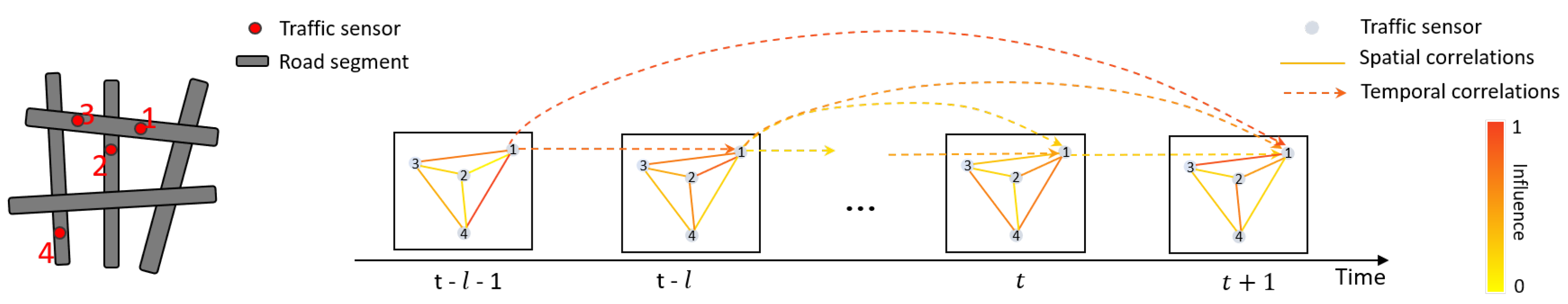
Factor 1: Global Spatial Dependencies. As shown in Figure 1, given the road network and sensors, the spatial correlations over different nodes on the traffic network are both local and global. Take Sensor 1 for example; the traffic status of its adjacent sensors (see Sensors 2 and 3) can influence that of Sensor 1. These are localized spatial correlations between sensors. In addition, the sensors (see Sensor 4) far from Sensor 1 can indirectly affect the traffic status of Sensor 1. Thus, all other sensors on the road network have impacts on Sensor 1. These are global spatial correlations between sensors.

Factor 2: Multiple Temporal Dependencies. Historical traffic conditions at different timestamps in the same location have different effects on status of a future timestamp. As shown by Sensor 1 in Figure 1, the traffic status at time $t+1$ is more related to that of time $t-l+1$, compared with that of time t. In addition, we find that the trend of traffic speed over time in different workdays shows a high degree of similarity in Figure 2a. Moreover, the trend of traffic speed on the same workday in different weeks is similar as well in Figure 2b, which indicates that traffic speed renders both short-term neighboring and multiple long-term periodic dependencies. Thus, we consider the recent, daily, and weekly periodic patterns for traffic speed prediction simultaneously.

Factor 3: External Factors. Traffic speed is significantly affected by external factors such as weather conditions, holidays, other special events, and so on. According to Figure 3a, it is clearly shown that the traffic speed on holidays is different from that on normal days. In addition, it can be seen in Figure 3b that the traffic speed of a heavily rainy day is much lower than that of a sunny day.

In addition to the above-mentioned key factors affecting traffic speed, there is uncertainty and inconsistency in the traffic data sensors collect, due to sensor failures, sensor maintenance, and other reasons. Several studies [2,3] have focused on evaluating and improving the reliability of sensors. To address the problem, in this paper, we also deal with the outliers and missing values in the traffic data, respectively.

Studies on traffic prediction have never stopped in the past few decades. Early statistical methods [4,5] and traditional machine learning methods [6,7,8] for traffic prediction cannot model the non-linear temporal correlations of traffic data effectively, and they hardly consider spatial dependencies. In recent years, with the continuous development of deep learning, many researchers have applied deep-learning-based methods to the traffic domain. Some studies [9,10,11] combine convolutional neural networks (CNNs) and recurrent neural networks (RNNs) for traffic prediction, where CNNs are used to capture the spatial dependencies while RNNs are used to extract the temporal correlations of traffic data.

The main limitation of the aforementioned methods is that conventional convolution operations only capture the spatial characteristics of regular grid structures. They are not suitable for data with irregular topologies. To tackle this problem, graph convolutional networks (GCNs) that can effectively handle non-Euclidean relations are integrated with RNNs [12] or CNNs [13] to embed prior knowledge of the road network and capture the correlations between sensors. The graph convolution network here represents the road network structure as a fixed weighted graph. Wu et al. [14] integrated Wavenet [15] into the GCN to capture the dynamic spatial-temporal correlations of traffic data, while using an adaptive adjacency matrix to obtain hidden spatial dependencies in the road network. However, there are still some limitations in these methods: (i) RNN-based models are challenging to train well [16] due to the problem of gradient disappearance or gradient explosion, and the receptive field of RNNs is limited; (ii) many existing methods only consider localized spatial correlations but ignore non-local ones; and (iii) they do not utilize more complicated traffic-related features such as the existing periodicity, repeating patterns, and external factors.

To capture the dynamic complex spatial-temporal correlations more effectively, we propose a novel global spatial-temporal graph convolutional network called GSTGCN to predict urban traffic speed, which consists of three independent spatial-temporal components with the same structure and one external component. Each spatial-temporal component contains a dynamic temporal module and a global correlated spatial module. The main contributions of this paper are as follows:

• We develop a dynamic temporal module, which consists of multiple residual blocks stacked by dilated causal convolutions. It has a long receptive field and can capture dynamic temporal correlations effectively.
• We design a global correlated spatial module, which contains a localized graph convolution and a global correlated mechanism. It is proposed to simultaneously capture the local spatial correlations and global ones between sensors in the traffic network.
• The whole model fuses the output of the three spatial-temporal components considering multiple temporal dependencies and takes external factors into account to predict traffic speed. The experimental results demonstrate that the proposed GSTGCN outperforms the eight baselines.

2. Related Work

Over the past few decades, traffic prediction has been extensively studied. Early statistical methods for traffic prediction were simple time series models, containing Autoregressive Integrated Moving Average (ARIMA) [4] and its variant [17], vector autoregression (VAR) [5], etc. These methods rely on data stationary assumption, thus have limited ability to model complex traffic data. Later, models based on traditional machine learning methods, such as k-nearest neighbors (KNN) [6], support vector regression (SVR) [7], and Kalman filtering (KF) [8], were applied to traffic prediction to model more complex data. However, these methods cannot capture non-linearity in traffic data effectively, and barely utilize spatial correlations [18]. Moreover, they need more detailed feature engineering.

Recently, methods based on deep learning have been applied in many fields and achieved success, which has inspired the study of traffic prediction to use deep-learning-based methods modeling the complex spatial-temporal dependencies of the traffic data [19]. Lv et al. [20] utilized a stacked autoencoder (SAE) to predict the traffic status of different nodes. Luo et al. [21] integrated KNN and LSTM [22] to predict traffic flow. Yu et al. [23] combined LSTM networks with SAE to predict traffic status in extreme conditions. Cui et al. [24] proposed a LSTM-based network composed of bidirectional ones and unidirectional ones for traffic prediction. In addition, Zhang et al. [25] transformed the road network into a regular 2D grid and used convolutional neural network to predict citywide crowd flows. Liu et al. [26] used fully-connected neural networks and improved residual network to predict bus traffic flow. Later, the authors of [9,10,11] combined convolutional neural networks (CNNs) with recurrent neural networks (RNNs) and its variants for traffic forecasting. However, the main limitation of the above models is that conventional convolution operations can only capture the spatial characteristics of regular grid structures but do not work for data points with irregular topologies. Therefore, they fail to make an effective use of the topological structure of the traffic network to capture complex spatial correlations.

To extract the spatial correlations of traffic data with complex topologies, extending neural networks to process graph-structured data has attracted widespread attention [27]. A series of studies has extended traditional convolution to model arbitrary graphs on spectral [28,29,30] or spatial [31,32,33] domain. Spectral-based methods use a graph spectral filter to smooth the input signals of nodes. Spatial-based methods extract high-level representations of nodes by gathering feature information of neighbors. Other studies focus on graph embedding, which learns low-dimensional representations for vertices that preserve the graph-structured information [34,35]. To overcome the limitation of conventional convolution and capture more complex spatial-temporal dependencies, Li et al. [12] proposed a framework that combines the diffusion convolutional with the recurrent neural network to forecast traffic conditions. Fang et al. [36] proposed Global Spatial-Temporal Network (GSTNet) for traffic flow prediction. GSTNet employs tensor casual convolution and global correlated mechanism for extracting dynamic temporal dependencies and global spatial correlations. Yu et al. [13] proposed the Spatio-Temporal GCN (ST-GCN), which uses a full convolution structure combining graph convolution with 1D convolution. In ST-GCN, the graph convolution is used to obtain the spatial correlation, and the 1D convolution is used to extract the temporal dependencies. STGCN is much more computationally efficiently than the above-mentioned models using RNNs. Afterward, ST-MetaNet [37] utilizes sequence-to-sequence structure and combines the graph attention network (GAT) with the recurrent neural network (RNN) for capturing the spatial-temporal correlations. Wu et al. [14] integrated Wavenet [15] into the GCN to extract the dynamic temporal dependencies of traffic data, while using an adaptive adjacency matrix to obtain hidden spatial dependencies in the road network. This self-adaptive adjacency matrix is constructed by the similarity of different node embeddings on the road network. However, the learned spatial dependencies between nodes lack the guidance of domain knowledge, and it is prone to overfit during the training phase [18]. In addition, most existing traffic speed prediction methods ignore global spatial correlations between different nodes in the road network, and they hardly utilize multiple temporal correlations and external factors.

3. Materials and Methods

3.1. Problem Description

The task of traffic speed prediction is to predict the future traffic speed based on the given historical traffic measurements (such as traffic speed, traffic flow, etc.) of observed sensors in the road network. We first define the road network as a weighted undirected graph $\mathcal{G}=(\mathcal{V},\mathcal{E},A)$, where $\mathcal{V}$ is a set of $\left|\mathcal{V}\right|=N$ nodes, representing observed sensors in the road network; $\mathcal{E}$ is a set of edges, indicating connectivity of nodes; and $A\in {\mathbb{R}}^{N\times N}$ is a weighted adjacency matrix, which represents the proximity between nodes and can be computed from the distance in the road network. Then, the traffic data observed at time t on $\mathcal{G}$ are denoted as a graph signal $X_t\in {\mathbb{R}}^{N\times F}$. Here, F represents the number of features observed at each node. The goal of traffic speed prediction is to learn a function f to predict future T graph signals based on graph $\mathcal{G}$ and $T^{\prime }$ historical graph signals:

$$X_{t+1},\dots ,X_{t+T}=f_{\theta }(X_{t-T^{\prime }+1},\dots ,X_t;\mathcal{G})$$

(1)

where $\theta$ stands for the learnable parameters.

3.2. The Architecture of Our Designed Network

Overview: As presented in Figure 4, the GSTGCN model proposed in this paper contains three independent spatial-temporal components with the same structure and an external component. The first three spatial-temporal components are designed to model the recent, daily-periodic, and weekly-periodic dependencies of the historical speed data, respectively, and the external component extracts the characteristics of external factors, such as weather condition, time of the day, and day of the week, to model external impacts on traffic speed. The first three spatial-temporal modules have the same structure. Each of them is composed of a temporal module with multiple stacked residual blocks and a global correlated spatial module. The global correlated spatial module models the localized spatial dependencies and the global spatial correlations of traffic data, respectively. We first construct an adjacency matrix based on the points of interest (POI) data around the sensors and the related features of the road segments. Then, we intercept three time series segments ${\mathcal{X}}_h$, ${\mathcal{X}}_d$, and ${\mathcal{X}}_w$ from the traffic data along the time axis as inputs to the three spatial-temporal components. Next, we extract the characteristics of external factors and enter them into the external component. After that, the outputs of the first three spatial-temporal components $Y_h$, $Y_d$, and $Y_w$ are assigned different weights and then fused into the output $Y_{res}$. Then, we merge the $Y_{res}$ with the output of the external component $Y_{ext}$ to generate the prediction result. Finally, we utilize a tanh function to map the result into $[-1,1]$ [38].

Adjacency Matrix Construction. Previous studies have only used the distances between sensors to construct the adjacency matrix, which represents the topological structure of the road network. However, even if two sensors are geographically far apart, they may have similar traffic conditions when they are in similar functional areas. Therefore, we consider not only the distance between the sensors, but also the similarity of the regions in which they are located to construct the adjacency matrix. More specifically, we first use the Dijkstra algorithm to calculate the distances between pairs of sensors in the road network, $dist(i,j)$ represents the distance between sensor i and sensor j. Next, we use Openstreetmap [39] mapping each sensor to the corresponding road segment and collect the properties of the segment as the road-related features of sensors, which includes speed _ limit, lanes, length, etc. Then, we obtain the number of points of interest (POIs) of ten categories within 500 m around the detector from FourSquare [40] as POI relevant features, which contain travel and transport, food, arts and entertainment, residence, etc. Finally, we splice the road-related features and POI data to form a feature vector $E^r$. The form is defined as:

$$E^r=(po{i}_1,\dots ,po{i}_{10},lanes,speed\_limit,type,length,is\_bridge,oneway)$$

(2)

where $po{i}_i$ is the number of points of interest of the ith category. The details of road-related features are presented in

Table 1. Road-related features.

Feature	Description
lanes	the number of lanes
speedLimit	speed limit of the road segment (km/h)
isBridge	whether the road leads to a bridge
roadLength	length of the road segment (km)
type	the type of road segment
oneway	whether roads allow driving in only one direction

. Therefore, we calculate the similarity of sensor i, j using the cosine similarity formula [41]:

$$sim(i,j)=\frac{{\displaystyle \sum _{m=1}^C}{E}_{i,m}^r\times E_{j,m}^r}{\parallel E_i^r\parallel \times \parallel E_j^r\parallel }$$

(3)

where C is the length of feature vector and $E_i^r$ represents the feature vector of sensor i. Finally, we use threshold-based Gaussian kernel [42] to calculate the adjacency matrix; the formula is as follows:

$$W_{i,j}=\left\{\begin{array}{cc}\begin{array}{c}{B}_{i,j}=w_{1}exp(-\frac{dist{(i,j)}^2}{2{\sigma }_1^2})+w_{2}exp(-\frac{{(1-sim(i,j))}^2}{2{\sigma }_2^2})\hfill \end{array}\hfill & \mathrm{if}{B}_{i,j}\ge \kappa \hfill \\ 0\hfill & \mathrm{otherwise}\hfill \end{array}\right.$$

(4)

where ${\sigma }_1$ is the standard deviation of distances; ${\sigma }_2$ is the standard deviation of similarities; $w_1+w_2=1$; and $\kappa$ is the threshold.

Detailed Three Time Series Segments: Suppose that the sampling frequency is p times a day. The current time is $t_0$, and the length of the sequence to be predicted is $T_p$. As described in Figure 5, we intercept three time series fragments of length $T_h$, $T_d$, and $T_w$ along the time axis as the inputs of three spatial-temporal components, respectively. Here, $T_h$, $T_d$, and $T_w$ are all integer multiples of $T_p$. The details of the three time series fragments are as follows:

• The recent segment:${\mathcal{X}}_h$ = ($X_{t_0-T_h+1}$, $X_{t_0-T_h+2}$, …, $X_{t_0}$)$\in {\mathbb{R}}^{N\times F\times T_h}$. As shown by the red part in Figure 5, this segment is directly adjacent to the time series to be predicted. Since the traffic condition of the sensors gradually spreads to the vicinity over time, the adjacent historical time series have a great impact on it.
• The daily-periodic segment:${\mathcal{X}}_d$ = ($X_{t_0-(T_d/T_p)\ast q+1}$, $X_{t_0-(T_d/T_p)\ast q+2}$, …, $X_{t_0-(T_d/T_p)\ast q+T_p}$, $X_{t_0-(T_d/T_p-1)\ast q+1}$, $X_{t_0-(T_d/T_p-1)\ast q+2}$, …, $X_{t_0-(T_d/T_p-1)\ast q+T_p}$, …, $X_{t_0-q+1}$, $X_{t_0-q+2}$, …, $X_{t_0-q+T_p}$)$\in {\mathbb{R}}^{N\times F\times T_d}$. It includes several time segments in the past few days that are the same as the predicted time period, as shown by the green part in Figure 5. As people’s daily routines are almost fixed on workdays, such as morning peaks and evening peaks, traffic data may show repeating patterns. The purpose of this component is to model the daily periodicity of traffic data.
• The weekly-periodic segment:${\mathcal{X}}_w$ = ($X_{t_0-(T_w/T_p)\ast 7\ast q+1}$, $X_{t_0-(T_w/T_p)\ast 7\ast q+2}$, …, $X_{t_0-(T_w/T_p)\ast 7\ast q+T_p}$, $X_{t_0-(T_w/T_p-1)\ast 7\ast q+1}$, $X_{t_0-(T_w/T_p-1)\ast 7\ast q+2}$, …, $X_{t_0-(T_w/T_p-1)\ast 7\ast q+T_p}$, …, $X_{t_0-q+1}$, $X_{t_0-q+2}$, …, $X_{t_0-q+T_p}$)$\in {\mathbb{R}}^{N\times F\times T_w}$. It is composed of the same periods of the past few weeks with the same week attribute as the time segment to be predicted, as shown by the blue part in Figure 5. Usually, the traffic pattern on a weekday is similar to those on the historical weekday, but the weekend would be different. The weekly-periodic component is designed to capture the weekly periodic patterns of traffic data.

3.3. Structures of the Three Spatial-Temporal Components

Traffic conditions usually involve multiple temporal periodic patterns, and the traffic data exhibit strong daily and weekly periodicity. Taking multiple periodic temporal dependencies into account will improve prediction performance [19]. The three spatial-temporal components, respectively, model the recent, daily-periodic, and weekly-periodic spatial-temporal dependencies with the same structure. It includes two sub-modules: a dynamic temporal module and a global correlated spatial module (see Figure 4).

3.3.1. Dynamic Temporal Module

We propose a dynamic temporal module to extract the temporal dependencies of the traffic data. The dynamic temporal module is composed of multiple residual blocks containing stacked dilated casual convolutions [43]. It has a long receptive field so as to capture both short-term neighboring and long-term periodic temporal dependencies with high effectiveness.

Dilated Casual Convolution: Dilated causal convolution (DCC) is based on 1D convolution, injecting holes into the convolution kernel, padding zeros to the input sequence to keep its length unchanged, skipping a fixed step, and sliding on the input sequence to operate convolution. In Figure 6, for a 1D sequence $x\in {\mathbb{R}}^T$ when the convolution kernel is $f\in {\mathbb{R}}^K$, $x_t$ denotes the tth value in the 1D sequence x, the dilated causal convolution is F, and the tth value of the dilated causal convolution result is as follows:

$$F_t\left(x\right)={\left(f{\ast }_{d}x\right)}_t=\sum _{i=0}^{K-1}f\left(i\right)·x_{t-d·i}$$

(5)

where d refers to the dilation factor. It is the distance skipped during the convolution process. Multiple stacked dilated casual convolutions with progressively increasing dilation factor $d^{\left(l\right)}=2^{(l-1)}$ make the model’s receptive field grow exponentially, where l denotes the number of layers.

Residual Block Architecture: As shown in Figure 4, a residual block contains two stacked dilated causal convolutional layers and an identity map. The identity map is connected across layers. It addresses the gradient explosion problem in the deep networks. Weight normalization [44] is added after each dilated causal convolution layer to tackle the overfitting problem. For non-linearity, the rectified linear unit (ReLU) [45] keeps the model’s convergence rate steady. The dilation factors of two DCC layers in a residual block are the same. Given an input $X^l\in {\mathbb{R}}^{N\times T\times F}$, the result $X^{l+1}\in {\mathbb{R}}^{N\times T\times F^{\prime }}$ after passing through the $(l+1)$th residual block is:

$$X^{l+1}=X^l+ReLU\left({\mathsf{\Phi }}_1{\ast }_{d_1}\left(ReLU\left({\mathsf{\Phi }}_0{\ast }_{d_0}{X}^l\right)\right)\right)$$

(6)

where ${\mathsf{\Phi }}_0$, ${\mathsf{\Phi }}_1\in {\mathbb{R}}^{F\times F^{\prime }\times K}$ are the convolution kernels for two dilated causal convolutions in a residual block. F and $F^{\prime }$ represent the number of input features and output channels, respectively; $d_0$ and $d_1$ are the dilation factors; and K is the length of the convolution kernel.

Most previous models used RNN- and CNN-based methods to capture temporal dependencies, but they cannot handle very long sequences and are prone to the problem of gradient explosions. In contrast, residual blocks have a larger receptive field via stacking fewer dilated casual convolutional layers, and the introduction of residual connections also eliminates the problem of gradient disappearance or explosion. Besides, this architecture can be calculated in parallel with much less resource consumption.

3.3.2. Global Correlated Spatial Module

This paper proposes a global correlated spatial module for capturing complex spatial correlations between nodes on the traffic network. The module contains a localized graph convolution and a global correlated mechanism with residual connection [16], where the former is used to extract local spatial correlations while the latter is used to capture the non-local spatial correlations.

Localized Graph Convolution: Since traditional convolutions fail to effectively extract the complicated spatial correlations between different nodes on the traffic network, the spectral graph theory extends the convolution to the graph-structured data. In spectral graph theory, the Laplacian matrix of a graph represents its topological structure. Therefore, we can study the properties of the graph by analyzing the eigenvalues and eigenvectors of the Laplacian matrix. The Laplacian matrix of a graph is defined as $\mathbf{L}=\mathbf{D}-\mathbf{A}$, and the normalized Laplacian matrix $\mathbf{L}={\mathbf{I}}_N-{\mathbf{D}}^{-\frac{1}{2}}\mathbf{A}{\mathbf{D}}^{-\frac{1}{2}}\in {\mathbb{R}}^{N\times N}$, where ${\mathbf{I}}_N$ is a unit matrix with N dimensions, $\mathbf{A}\in {\mathbb{R}}^{N\times N}$ is the adjacency matrix, and the $\mathbf{D}\in {\mathbb{R}}^{N\times N}$ is the degree matrix, with ${\mathbf{D}}_{ii}={\sum }_j{\mathbf{A}}_{ij}$. The eigenvalue decomposition of the normalized Laplacian matrix is $\mathbf{L}=\mathbf{U}\mathbf{\Lambda }{\mathbf{U}}^T$, where $\mathbf{U}$ is eigenvectors of the normalized $\mathbf{L}$ and $\mathbf{\Lambda }$ is the diagonal matrix with corresponding eigenvalues. Let $\mathit{x}\in {\mathbb{R}}^N$ be the signal of all nodes on the traffic network. The Fourier transform of the signal $\mathit{x}$ is $\widehat{\mathit{x}}={\mathbf{U}}^T\mathit{x}$. According to the properties of the Laplacian matrix, $\mathbf{U}$ is an orthogonal matrix, so the inverse Fourier transform of the signal $\widehat{\mathit{x}}$ is $\mathit{x}=\mathbf{U}\widehat{\mathit{x}}$. Based on these concepts, the signal $\mathit{x}$ on graph $\mathbf{G}$ is filtered by the convolution kernel $g_{\theta }$:

$$g_{\theta }{\ast }_{\mathbf{G}}\mathit{x}=g_{\theta }\left(\mathbf{L}\right)\mathit{x}=g_{\theta }(\mathbf{U}\mathbf{\Lambda }{\mathbf{U}}^T)\mathit{x}=\mathbf{U}{g}_{\theta }(\mathbf{\Lambda }){\mathbf{U}}^T\mathit{x}$$

(7)

The spectral graph convolution first uses the Fourier transform to map the graph signal $\mathit{x}$ and the kernel $g_{\theta }$ into an orthogonal space formed by the Laplacian matrix eigenvectors, then performs convolution in the Fourier domain, and last conducts the inverse Fourier transform to obtain the final graph convolution results. However, this method requires explicit Laplacian matrix eigenvalue decomposition, and the computational complexity is too high, when the scale of the graph is large. Therefore, in this paper, we employ the Chebyshev polynomial [29] to approximate the convolution kernel and solve this problem. The formula is as follows:

$$g_{\theta }{\ast }_{\mathbf{G}}\mathit{x}=g_{\theta }\left(\mathbf{L}\right)\mathit{x}=\sum _{k=0}^{K-1}{\theta }_k{T}_k\left(\tilde{\mathbf{L}}\right)\mathit{x}$$

(8)

where the parameter $\theta \in {\mathbb{R}}^K$ is a vector of polynomial coefficients and $\tilde{\mathbf{L}}=\frac{2}{{\lambda }_{max}}\mathbf{L}-{\mathbf{I}}_N$, with ${\lambda }_{max}$ the maximal eigenvalue of the Laplacian matrix. The Chebyshev polynomials are recursively defined as $T_k\left(\mathit{x}\right)=2\mathit{x}{T}_{k-1}\left(\mathit{x}\right)-T_{k-2}\left(\mathit{x}\right)$, in which $T_0\left(\mathit{x}\right)=1$, $T_1\left(\mathit{x}\right)=\mathit{x}$.

We denote $x_{i,t}\in {\mathbb{R}}^C$ as all extracted features of the ith node at the tth historical timestamp, where C is the number of the input channels. Thus, the input signal of the graph convolution is a feature matrix ${\mathit{X}}_t={[{\mathit{x}}_{1,t},{\mathit{x}}_{2,t},\dots ,{\mathit{x}}_{N,t}]}^T\in {\mathbb{R}}^{N\times C}$ and the result of graph convolution is as follows:

$${\widehat{\mathit{X}}}_t=\sum _{k=0}^{K-1}{\theta }_k{T}_k\left(\tilde{\mathbf{L}}\right){\mathit{X}}_t$$

(9)

where ${\widehat{\mathit{X}}}_t=[{\widehat{\mathit{x}}}_{1,t},{\widehat{\mathit{x}}}_{2,t},\dots ,{\widehat{\mathit{x}}}_{N,t}]\in {\mathbb{R}}^{N\times D}$, and D is the number of the output channels. It is worth noting that the convolution results contain the feature information of K-order neighbors, and only capture the local spatial correlation of the road network structure.

Global Correlated Spatial Mechanism: To model the global spatial correlations between different nodes in the road network, a global correlated mechanism is proposed, as depicted in Figure 4. The formula for computing global correlations is as follows:

$${\mathit{y}}_{i,t}=\sum _{\forall v_j\ne v_i}{s}_{i,j}·\varphi ({\widehat{\mathit{x}}}_{i,t},{\widehat{\mathit{x}}}_{j,t})·{\widehat{\mathit{x}}}_{j,t}{W}_g+{\widehat{\mathit{x}}}_{i,t}{W}_r$$

(10)

where ${\mathit{y}}_{i,t}\in {\mathbb{R}}^F$ represents the output feature of the ith node at timestamp t. Considering whether there is an edge between the ith node and the jth node in the road network, if there is an edge, $s_{i,j}=\alpha >1$, else $s_{i,j}$ = 1. $s_{i,j}$ represents the static global topological weights. In Equation (10), $\varphi$ is the Gaussian kernel $\varphi (\mathit{x},\mathit{y})=exp\left({\mathit{x}}^T{W}_{\varphi }\mathit{y}\right)$, measuring the correlations between two node embedding representations, where $W_{\varphi }\in {\mathbb{R}}^{D\times D}$ is the learnable parameter. ${\sum }_{\forall v_j\ne v_i}{s}_{i,j}·\varphi ({\widehat{\mathit{x}}}_{i,t},{\widehat{\mathit{x}}}_{j,t})·{\widehat{\mathit{x}}}_{j,t}{W}_g$ represents the impact of all other nodes on the ith node in the spatial dimension and “$+{\widehat{\mathit{x}}}_{i,t}{W}_r$” denotes a residual connection with the localized output features of the ith node, with $W_r\in {\mathbb{R}}^{D\times F}$ and $W_g\in {\mathbb{R}}^{D\times F}$ the learnable parameters. The output of the global correlated mechanism at timestamp t is ${\mathit{Y}}_t={[{\mathit{y}}_{1,t},{\mathit{y}}_{2,t},\dots ,{\mathit{y}}_{N,t}]}^T\in {\mathbb{R}}^{N\times F}$, and the final output feature matrix of the spatial module is $Y\in {\mathbb{R}}^{N\times T\times F}$.

3.4. The Structure of the External Component

Traffic speed is affected by many factors such as holidays, weather conditions, and so on. Suppose $t_0$ is the current time and $S_{t+1}$ represents the feature vector of the external factor at time interval $t+1$ to be predicted. We use the feature vectors of the T time intervals to form a feature matrix S. In our implementation, $S={[S_{t+1},\dots ,S_{t+T}]}^T\in {\mathbb{R}}^{T\times F_s}$, where $F_s=15$ is the number of features we select. Specific details are shown in

Table 2. External factors.

Name	Description
is_weekend	whether it is weekend, dimension: 1
is_weekday	whether it is weekday, dimension: 1
is_holiday	whether it is holiday, dimension: 1
hour	hour of the time, dimension: 1
minute	minute of the time, dimension: 1
weather	e.g., clear-day, rain, cloudy, dimension: 10

. Since the weather conditions at the next T intervals are unknown, we use the weather forecasting data from the weather website Darksky [46]. Next, we stack two fully-connected layers in the external component to deal with the external factor features. The first layer embeds each sub-factor and followed by an activation. The second layer maps the low-dimensional features to the higher-dimensional ones to get ${\mathit{Y}}_{ext}$ whose shape is the same as ${\mathit{Y}}_{res}$.

3.5. Multi-Component Fusion

In this section, we discuss how to integrate the four main parts of the model. Since the first three spatiotemporal components model the recent, daily-periodic, and weekly-periodic spatial-temporal correlations, respectively, the impact of the three parts on different locations is various. For example, we intend to predict the traffic speed at 08:30 on Monday morning. For some places with obvious morning peaks, the output of the daily-periodic and weekly-periodic component have significant impacts on prediction performance, and for some places where there is no obvious periodic pattern, the output of the daily component and weekly component will be useless. Above all, the different locations are all affected by short-term neighbors, long-term period, and trend, but the degrees of impact may be diverse [25]. Therefore, the impact weights of different spatiotemporal components on each node are constantly changing, and these weight values should be learned from historical traffic data. Thus, we fuse the three components of Figure 4 as follows:

$${\mathit{Y}}_{res}=W_h\circ {\mathit{Y}}_h+W_d\circ {\mathit{Y}}_d+W_w\circ {\mathit{Y}}_w$$

(11)

where ∘ is Hadamard product. $W_h$, $W_d$, and $W_w$ are all learned parameters. These parameters indicate the degree to which the outputs of the three spatiotemporal components affect the forecasting target.

Then, we further merge the fusion result ${\mathit{Y}}_{res}$ of the three spatiotemporal components with the output of the external component ${\mathit{Y}}_{ext}$ to generate the final prediction result $\widehat{\mathit{Y}}$, as illustrated in Figure 4. The output of the entire model is:

$$\widehat{\mathit{Y}}=tanh({\mathit{Y}}_{res}+{\mathit{Y}}_{ext})$$

(12)

where tanh is a function to map the prediction result to the range of $[-1,1]$ and makes the model converge faster.

Our model predicts the future T timestamps speeds of all sensors based on the historical $T^{\prime }$ traffic conditions. We choose the L2 loss as the training target of GSTGCN, which is defined by:

$$L({\widehat{\mathit{Y}}}_{t+1},\dots ,{\widehat{\mathit{Y}}}_{t+T};\Theta )=\sum _t\sum _{i=1}^T\parallel {\widehat{\mathit{Y}}}_{t+i}-{\mathit{Y}}_{t+i}{\parallel }^2$$

(13)

where $\Theta$ are all learnable parameters in the GSTGCN, ${\mathit{Y}}_{t+i}$ is the ground truth, and ${\widehat{\mathit{Y}}}_{t+i}$ is the model’s prediction result.

4. Experiments

4.1. Datasets

The proposed model was verified on two highway traffic datasets, PeMSD4 and PeMSD7, collected by Caltrans Performance Measurement System (PeMS) [47] at 30-s intervals. The traffic speed data were aggregated from the raw data into 5-min windows. This system deploys 39,000 detectors in major cities in California. Geographic information of sensors is recorded in datasets with corresponding interval. The details of the datasets in our experiments are:

PeMSD7: It contains the traffic information from the sensors on the highways of Los Angeles County. We selected 204 sensors and collected three months of data from 1 January 2018 to 31 March 2018 for the experiment.

PeMSD4: It refers to the traffic data from the sensors in San Francisco Bay Area. We chose 325 sensors and extracted the data from 1 January 2017 to 31 March 2017 for the experiment.

During the experiment, both datasets were divided into chronological order, with 70% used for training, 10% for validation, and the remaining 20% for testing. The sensors distribution of the two datasets is displayed in Figure 7. In the data preprocessing stage, we discarded traffic speed outliers less than 0 and used the tensor decomposition method to complete the missing values in the traffic speed data. Then, we encoded the non-numeric features in external factors using a one-hot encoding scheme. Later, we used Min-Max normalization to map its value into $[0,1]$ and the original speed into $[-1,1]$. During the evaluation phase, we re-projected the speed back to the original range as the final prediction result.

4.2. Evaluation Metric

In the experiments, we applied three widely-used metrics to evaluate the performance of our model: Mean Absolute Error (MAE), Root Mean Squared Error (RMSE) and Mean Absolute Percentage Error (MAPE). They are defined as follows:

$$MAE=\frac{1}{M\times N}\sum _{i=1}^M\sum _{j=1}^N|{\mathit{y}}_{i,j}-{\widehat{\mathit{y}}}_{i,j}|$$

(14)

$$RMSE=\sqrt{\frac{1}{M\times N}\sum _{i=1}^M\sum _{j=1}^N{({\mathit{y}}_{i,j}-{\widehat{\mathit{y}}}_{i,j})}^2}$$

(15)

$$MAPE=\frac{1}{M\times N}\sum _{i=1}^M\sum _{j=1}^N\frac{|{\mathit{y}}_{i,j}-{\widehat{\mathit{y}}}_{i,j}|}{{\mathit{y}}_{i,j}}$$

(16)

where ${\widehat{\mathit{y}}}_{i,j}$ and ${\mathit{y}}_{i,j}$ are the true value and the predicted value, N is the number of detectors we select in the road network, and M is the total number of predicted samples.

4.3. Baselines

We compared our model with the following eight models:

• ARIMA [4]: This model predicts future time series data based on historical series values.
• SVR [7]: This model uses support vector regression to predict travel time.
• SAE [20]: A stacked auto-encoder model is used to learn common traffic flow features and is trained in a voraciously layered way.
• SBU-LSTM [24]: A deep LSTM-based network composed of bidirectional ones and unidirectional ones for traffic prediction.
• DCRNN [12]: Diffusion Convolutional Recurrent Neural Network integrates sequence2sequence framework and diffusion convolution to model the relationships of inflow and outflow.
• STGCN [13]: Spatio-Temporal Graph Convolutional Network is a complete convolutional structure combining graph convolution with 1D standard convolution layers for traffic prediction.
• ST-MetaNet [37]: Spatial-Temporal Meta Learning Network utilizes graph attention network (GAT) and the recurrent neural network (RNN) for traffic prediction.
• Graph WavaNet [14]: Graph WavaNet employs graph convolution network (GCN) with self-adaptive matrix and a stacked dilated 1D convolution to model the spatial-temporal graph.

4.4. Experiment Settings

We implemented our GSTGCN model based on the Pytorch framework and conducted experiments on a computer with one Intel(R) Xeon(R) W-2123 CPU @ 3.60GHz and one NVIDIA Quadro P2000 GPU card. The dynamic temporal module in the model contained four residual blocks. The residual blocks consisted of two stacked dilated casual convolutions. The kernel size was set as 3. The dilation factors of three residual blocks were 1, 2, and 4. The number of kernels in localized graph convolution and the hidden channels was set to 8. The hyperparameter $\alpha$ was set as 2. For external component, we set the output channels of the first fully-connected layer to 22, and the output channels were reduced to 1 by the next fully-connected layer. During the phase of constructing adjacency matrix, $\kappa$, $w_1$ and $w_2$ were set as 0.5. The batch size was 256, and we trained the model for 30 epochs. We used Adam optimizer to train our model with the initialized learning rate of 0.001. During the testing phase, we predicted the traffic speed in the next hour (12 steps) based on 12 historical speeds.

4.5. Experimental Results

4.5.1. Prediction Performance Comparison

Table 3. Performance comparison of different approaches for traffic prediction on PeMSD7 and PeMSD4 datasets. The best results are marked in bold.

Data	Method	15 min			30 min			1 h
		MAE	RMSE	MAPE	MAE	RMSE	MAPE	MAE	RMSE	MAPE
PeMSD7	ARIMA	5.68	9.38	12.36%	6.29	9.98	13.67%	7.23	11.02	14.52%
	SVR	3.67	5.52	7.64%	4.28	8.02	9.19%	5.14	9.67	11.27%
	SAE	3.44	5.25	7.24%	4.01	7.89	8.89%	4.92	9.25	10.43%
	SBU-LSTM	3.52	5.05	7.01%	3.95	7.42	8.52%	4.78	8.93	9.87%
	DCRNN	2.46	4.52	5.50%	3.32	6.51	7.94%	4.37	8.23	8.78%
	STGCN	2.34	4.40	5.36%	3.28	6.34	7.80%	4.16	7.86	8.80%
	ST-MetaNet	2.05	3.95	4.52%	2.81	5.66	6.23%	3.57	7.10	8.01%
	Graph WaveNet	2.04	3.92	4.72%	2.74	5.54	6.83%	3.36	6.74	8.74%
	GSTGCN	1.20	2.16	2.66%	1.81	3.03	4.58%	3.05	4.63	8.63%
PeMSD4	ARIMA	5.04	7.45	10.86%	6.06	8.09	11.05%	6.98	9.78	12.32%
	SVR	3.08	4.62	6.54%	4.09	6.72	7.78%	5.67	8.13	10.96%
	SAE	2.90	4.44	6.25%	3.98	6.48	7.52%	5.28	7.66	8.34%
	SBU-LSTM	2.10	4.01	6.09%	3.66	6.26	7.05%	4.33	6.85	7.88%
	DCRNN	2.15	3.45	4.38%	2.90	5.15	5.74%	3.49	5.78	6.17%
	STGCN	2.05	3.30	4.27%	2.85	4.98	5.65%	3.24	5.65	5.98%
	ST-MetaNet	1.21	2.73	4.01%	1.79	4.17	3.92%	2.31	5.12	4.83%
	Graph WaveNet	1.31	2.76	2.75%	1.66	3.75	3.69%	2.00	4.61	4.73%
	GSTGCN	0.73	1.65	1.78%	1.31	3.17	2.94%	1.89	3.43	4.78%

displays the GSTGCN and all baseline models on the PeMSD4 and PeMSD7 datasets for prediction of MAE, RMSE, and MAPE of 15 min (3 steps), 30 min (6 steps), and 60 min (12 steps). As shown in the table, we observed that deep learning methods perform better than simple time series methods (ARIMA) and traditional machine learning methods (SVR), indicating that deep learning methods can model more complex traffic data. Graph-based models containing STGCN, DCRNN, Graph WaveNet, ST-MetaNet, and GSTGCN predict more accurately than SAE and SBU-LSTM. It means that the spatial topological information of the traffic data is critical to prediction performance. Compared to DCRNN, STGCN, ST-MetaNet, and Graph WaveNet, GSTGCN has a great advantage in long-term prediction with a slower error growth rate and achieves the best prediction accuracy on all metrics and both two datasets. To further verify the accuracy of our model, we compared the prediction performance of GSTGCN for the morning peak hours and weekends with that of Graph Wavenet. Based on the experimental result shown in Figure 8, we found that GSTGCN performs better than Graph WaveNet, which demonstrates that GSTGCN is more effective in modeling the complex spatiotemporal correlations.

4.5.2. Model Structure Comparison

In this section, we mainly discuss the structural differences between STGCN [13], ST-MetaNet [37], Graph WaveNet [14], and our proposed model GSTGCN.

STGCN is a deep learning framework with complete convolutional structures. It contains multiple 1D casual convolutions followed by a gated linear unit (GLU) for capturing temporal correlations and employs K-order Chebyshev graph convolution on traffic data to extract spatial dependencies. The architecture only captures simple nonlinear temporal correlations and localized spatial dependencies of traffic data. We can observe that STGCN performs poorly compared to the other models in Figure 9a, especially in the case of long-term prediction.

ST-MetaNet employs a sequence-to-sequence architecture. It introduces meta-learning to spatiotemporal modeling. The model first utilizes the points of interests (POIs) and density of road network around the detector to construct node attributes and then constructs the graph’s edge attributes using k-nearest neighbor (KNN) algorithm. In the model, a meta graph attention network (GAT) is used to capture diverse spatial correlations, and a meta recurrent neural network (RNN) is employed to consider diverse temporal correlations. Compared with the ordinary 1D casual convolution, RNN has the advantage for time series modeling, as it can remember the previous input sequence using its inner memory structure. Besides, ST-MetaNet takes meta-learning knowledge into account. Thus, it is superior to STGCN in Table 3 and Figure 9a.

Graph WaveNet is a graph neural network architecture for spatial-temporal graph modeling. In the spatial dimension, Graph WaveNet introduces an adaptive adjacency matrix to capture spatial correlation based on diffusion convolution. The adaptive adjacency could learn the hidden spatial dependency existing in the road network and the diffusion convolution could capture localized spatial correlations. In the temporal dimension, Graph WaveNet employs stacked dilated casual convolution (DCC) to obtain temporal dependencies. The stacked dilated casual convolution’s receptive field grows exponentially as the number of layers increases and can handle long sequence very well. Therefore, as shown in Table 3 and Figure 9a, Graph WaveNet performs better than ST-MetaNet.

Our proposed model GSTGCN integrates the spatiotemporal correlations of traffic data and the influence of external factors together. In the temporal dimension, we employ three spatial-temporal components considering multiple temporal periodicities, and we use stacked dilated casual convolution (DCC) with residual connection to obtain temporal dynamics in each component. In the spatial dimension, we model local and global correlations through a global correlated module, which contains K-order Chebyshev graph convolution and a global correlated mechanism. When constructing the adjacency matrix, we consider not only the distance between the geographic locations of the sensors, but also the surrounding points of interests (POIs) data to explore the functional similarity of the area where the sensors are located. In addition, we take external factors into account using fully connected layers. Compared to Graph WaveNet, GSTGCN considers multiple temporal periodicities, global spatial correlations, and the impact of external factors on traffic data. Hence, the experimental results demonstrate that GSTGCN achieves the best prediction accuracy on all metrics.

4.5.3. Number of Residual Blocks in Dynamic Temporal Module

To determine the appropriate number of residual blocks in the model, we selected different numbers of residual blocks and performed experiments. The experimental results are presented in Figure 10a. As the number of residual blocks increases, the prediction performance of the model improves. However, after the number of residual blocks reaches 4, the accuracy of the model does not continue to improve or even becomes worse, and the training time of the model also increases greatly. Finally, four residual blocks are used in the dynamic temporal module of our model.

4.5.4. Effect of Each Component

To investigate the effect of each component of our model on the prediction result, we evaluate the four variants separately by removing the external module, the global correlated mechanism, the independent daily-periodic spatial-temporal component, and the independent weekly-periodic spatial-temporal component from GSTGCN. These four variants are: GSTGCN-noExt, GTSGCN-noGlo, GSTGCN-noDay, and GSTGCN-noWeek. Figure 10b illustrates the MAE comparison of the GSTGCN and its four variants predicting the next 12 steps on PeMSD7. It can be seen from the figure that the GSTGCN consistently outperforms GSTGCN-noExt and GSTGCN-noGlo, indicating the effectiveness of the external component and the global correlated mechanism. The other two models, GSTGCN-noDay and GSTGCN-noWeek, have similar short-term prediction performance as GSTGCN, but they perform worse in the long-term predictions. Therefore, it is proved that the daily-periodic component and the weekly-periodic component help to capture the long-term temporal dependencies of the traffic data more effectively.

4.5.5. Fault Tolerance Comparison

Due to sensor maintenance and breakdown, there are partially missing values in the traffic data. To evaluate the fault-tolerant ability of the model, we randomly discarded a fraction $\alpha$ of the historical traffic data, and trained the model using the remaining data. In the experiment, we set the $\alpha$ ranging from 10% to 90%. We conducted experiments on the GSTGCN, Graph Wavenet, DCRNN, STGCN, and ST-MetaNet using the dataset PeMSD7 separately, and the prediction MAE are shown in Figure 9b. Our proposed model, GSTGCN, has better fault tolerance than all the other baselines. It indicates that GSTGCN learn complex spatiotemporal correlations more effectively from sparse and noisy real-world datasets.

4.5.6. Training Efficiency

We compared the computational cost of GSTGCN, DCRNN, STGCN, ST-Metanet, and Graph WaveNet on PeMSD7. For the sake of fairness, the training time is the time it takes each model to train one epoch, and the inference time is the time cost of each model to predict the traffic speed at 12 timestamps in the next hour on the validation data.

Table 4. The computation time on the PeMSD7 dataset.

Model	GSTGCN	Graph WaveNet	ST-MetaNet	STGCN	DCRNN
Training time (s/epoch)	117.01	520.71	825.52	185.27	1378.25
Inference time (s)	16.32	23.68	44.55	118.597	253.64

demonstrates the experiment results. We observed that, during the training phase, the fastest is GSTGCN, followed by STGCN and Graph WaveNet. GSTGCN runs eleven times faster than DCRNN and seven times faster than ST-MetaNet in training. Since DCRNN and ST-MetaNet use recurrent neural network to capture temporal dependencies, they need more time to train. For inference, GSTGCN is the most effective one, and the time cost of STGCN and DCRNN significantly increases because they need to iteratively predict the results of 12 steps, while GSTGCN and Graph WaveNet generate 12 predictions in one run. To further investigate the performance of the compared models, we plot the Mean RMSE of 12 steps on the PeMSD7 test set with increasing training epochs, as shown in Figure 9a. The figure suggests that our GSTGCN achieves easier convergence and faster training procedure.

5. Conclusions

We propose a novel global spatial-temporal graph convolutional network called GSTGCN to predict urban traffic speed. In the spatial dimension, the model combines localized graph convolution and global correlated mechanism for local and non-local spatial correlations. When constructing the adjacency matrix that represents the structure of the road network, the model considers not only the distances between the sensors, but also the similarities of the sensors’ locations. In the temporal dimension, three independent modules are used to model the recent, daily-periodic and weekly-periodic temporal dependencies, respectively. Each module consists of several residual blocks containing stacked dilated causal convolutions. In addition, the model takes the effects of weather condition and other factors such as holidays into account. Experiments on two real-world datasets showed that the prediction accuracy of our model GSTGCN is significantly better than existing models. In the future work, we plan to explore more complex spatial correlations to further improve the prediction accuracy. Since GSTGCN is a general framework for the spatiotemporal prediction problem of graph-structured data, we can also apply it to other practical applications, such as arrival time estimation.

References

- Artuñedo, A.; Del Toro, R.M.; Haber, R.E. Consensus-based cooperative control based on pollution sensing and traffic information for urban traffic networks. Sensors 2017, 17, 953. [Google Scholar] [CrossRef] [Green Version]
- Castaño, F.; Strzelczak, S.; Villalonga, A.; Haber, R.E.; Kossakowska, J. Sensor Reliability in Cyber-Physical Systems Using Internet-of-Things Data: A Review and Case Study. Remote Sens. 2019, 11, 2252. [Google Scholar] [CrossRef] [Green Version]
- Castaño, F.; Beruvides, G.; Villalonga, A.; Haber, R.E. Self-tuning method for increased obstacle detection reliability based on internet of things LiDAR sensor models. Sensors 2018, 18, 1508. [Google Scholar] [CrossRef] [PubMed] [Green Version]
- Makridakis, S.; Hibon, M. ARMA models and the Box–Jenkins methodology. J. Forecast. 1997, 16, 147–163. [Google Scholar] [CrossRef]
- Zivot, E.; Wang, J. Vector autoregressive models for multivariate time series. In Modeling Financial Time Series with S-Plus®; Springer: New York, NY, USA, 2006; pp. 385–429. [Google Scholar]
- Zheng, Z.; Su, D. Short-term traffic volume forecasting: A k-nearest neighbor approach enhanced by constrained linearly sewing principle component algorithm. Transp. Res. Part Emerg. Technol. 2014, 43, 143–157. [Google Scholar] [CrossRef] [Green Version]
- Wu, C.H.; Ho, J.M.; Lee, D.T. Travel-time prediction with support vector regression. IEEE Trans. Intell. Transp. Syst. 2004, 5, 276–281. [Google Scholar] [CrossRef] [Green Version]
- Lippi, M.; Bertini, M.; Frasconi, P. Short-term traffic flow forecasting: An experimental comparison of time-series analysis and supervised learning. IEEE Trans. Intell. Transp. Syst. 2013, 14, 871–882. [Google Scholar] [CrossRef]
- Du, S.; Li, T.; Gong, X.; Yu, Z.; Huang, Y.; Horng, S.J. A hybrid method for traffic flow forecasting using multimodal deep learning. arXiv 2018, arXiv:1803.02099. [Google Scholar] [CrossRef] [Green Version]
- Yao, H.; Tang, X.; Wei, H.; Zheng, G.; Yu, Y.; Li, Z. Modeling spatial-temporal dynamics for traffic prediction. arXiv 2018, arXiv:1803.01254. [Google Scholar]
- Yao, H.; Wu, F.; Ke, J.; Tang, X.; Jia, Y.; Lu, S.; Gong, P.; Ye, J.; Li, Z. Deep multi-view spatial-temporal network for taxi demand prediction. In Proceedings of the Thirty-Second AAAI Conference on Artificial Intelligence, New Orleans, LA, USA, 2–7 February 2018. [Google Scholar]
- Li, Y.; Yu, R.; Shahabi, C.; Liu, Y. Diffusion Convolutional Recurrent Neural Network: Data-Driven Traffic Forecasting. In Proceedings of the International Conference on Learning Representations (ICLR ’18), Vancouver, BC, Canada, 30 April–3 May 2018. [Google Scholar]
- Yu, B.; Yin, H.; Zhu, Z. Spatio-temporal Graph Convolutional Networks: A Deep Learning Framework for Traffic Forecasting. In Proceedings of the 27th International Joint Conference on Artificial Intelligence (IJCAI), Stockholm, Sweden, 13–19 July 2018. [Google Scholar]
- Wu, Z.; Pan, S.; Long, G.; Jiang, J.; Zhang, C. Graph WaveNet for Deep Spatial-Temporal Graph Modeling. arXiv 2019, arXiv:1906.00121. [Google Scholar]
- Oord, A.V.D.; Dieleman, S.; Zen, H.; Simonyan, K.; Vinyals, O.; Graves, A.; Kalchbrenner, N.; Senior, A.; Kavukcuoglu, K. Wavenet: A generative model for raw audio. arXiv 2016, arXiv:1609.03499. [Google Scholar]
- He, K.; Zhang, X.; Ren, S.; Sun, J. Deep residual learning for image recognition. In Proceedings of the IEEE Conference on Computer Vision and Pattern Recognition, Las Vegas, NV, USA, 27–30 June 2016; pp. 770–778. [Google Scholar]
- Chen, J.; Li, D.; Zhang, G.; Zhang, X. Localized space-time autoregressive parameters estimation for traffic flow prediction in urban road networks. Appl. Sci. 2018, 8, 277. [Google Scholar] [CrossRef] [Green Version]
- Chen, W.; Chen, L.; Xie, Y.; Cao, W.; Gao, Y.; Feng, X. Multi-Range Attentive Bicomponent Graph Convolutional Network for Traffic Forecasting. arXiv 2019, arXiv:1911.12093. [Google Scholar]
- Yao, H.; Tang, X.; Wei, H.; Zheng, G.; Li, Z. Revisiting spatial-temporal similarity: A deep learning framework for traffic prediction. In Proceedings of the AAAI Conference on Artificial Intelligence, Hawaii, HI, USA, 27 January–1 February 2019. [Google Scholar]
- Lv, Y.; Duan, Y.; Kang, W.; Li, Z.; Wang, F.Y. Traffic flow prediction with big data: A deep learning approach. IEEE Trans. Intell. Transp. Syst. 2014, 16, 865–873. [Google Scholar] [CrossRef]
- Luo, X.; Li, D.; Yang, Y.; Zhang, S. Spatiotemporal traffic flow prediction with KNN and LSTM. J. Adv. Transp. 2019, 2019, 4145353. [Google Scholar] [CrossRef] [Green Version]
- Hochreiter, S.; Schmidhuber, J. Long short-term memory. Neural Comput. 1997, 9, 1735–1780. [Google Scholar] [CrossRef]
- Yu, R.; Li, Y.; Shahabi, C.; Demiryurek, U.; Liu, Y. Deep learning: A generic approach for extreme condition traffic forecasting. In Proceedings of the 2017 SIAM International Conference on Data Mining, Houston, TX, USA, 27–29 April 2017; pp. 777–785. [Google Scholar]
- Cui, Z.; Ke, R.; Wang, Y. Deep stacked bidirectional and unidirectional LSTM recurrent neural network for network-wide traffic speed prediction. In Proceedings of the 6th International Workshop on Urban Computing (UrbComp 2017), Halifax, NS, Canada, 14 August 2017. [Google Scholar]
- Zhang, J.; Zheng, Y.; Qi, D. Deep spatio-temporal residual networks for citywide crowd flows prediction. In Proceedings of the Thirty-First AAAI Conference on Artificial Intelligence, San Francisco, CA, USA, 4–9 February 2017. [Google Scholar]
- Liu, P.; Zhang, Y.; Kong, D.; Yin, B. Improved Spatio-Temporal Residual Networks for Bus Traffic Flow Prediction. Appl. Sci. 2019, 9, 615. [Google Scholar] [CrossRef] [Green Version]
- Wu, Z.; Pan, S.; Chen, F.; Long, G.; Zhang, C.; Yu, P.S. A comprehensive survey on graph neural networks. arXiv 2019, arXiv:1901.00596. [Google Scholar]
- Bruna, J.; Zaremba, W.; Szlam, A.; LeCun, Y. Spectral networks and locally connected networks on graphs. arXiv 2013, arXiv:1312.6203. [Google Scholar]
- Defferrard, M.; Bresson, X.; Vandergheynst, P. Convolutional neural networks on graphs with fast localized spectral filtering. In Advances in Neural Information Processing Systems; Neural Information Processing Systems (NIPS): Barcelona, Spain, 2016; pp. 3844–3852. [Google Scholar]
- Kipf, T.N.; Welling, M. Semi-supervised classification with graph convolutional networks. arXiv 2016, arXiv:1609.02907. [Google Scholar]
- Atwood, J.; Towsley, D. Diffusion-convolutional neural networks. In Advances in Neural Information Processing Systems; Neural Information Processing Systems (NIPS): Barcelona, Spain, 2016; pp. 1993–2001. [Google Scholar]
- Gilmer, J.; Schoenholz, S.S.; Riley, P.F.; Vinyals, O.; Dahl, G.E. Neural message passing for quantum chemistry. In Proceedings of the 34th International Conference on Machine Learning, Sydney, Australia, 6–11 August 2017; Volume 70, pp. 1263–1272. [Google Scholar]
- Hamilton, W.; Ying, Z.; Leskovec, J. Inductive representation learning on large graphs. In Advances in Neural Information Processing Systems; Neural Information Processing Systems (NIPS): Long Beach, CA, USA, 2017; pp. 1024–1034. [Google Scholar]
- Grover, A.; Leskovec, J. node2vec: Scalable feature learning for networks. In Proceedings of the 22nd ACM SIGKDD International Conference on Knowledge Discovery and Data Mining, San Francisco, CA, USA, 13–17 August 2016; pp. 855–864. [Google Scholar]
- Cui, P.; Wang, X.; Pei, J.; Zhu, W. A survey on network embedding. IEEE Trans. Knowl. Data Eng. 2018, 31, 833–852. [Google Scholar] [CrossRef] [Green Version]
- Fang, S.; Zhang, Q.; Meng, G.; Xiang, S.; Pan, C. Gstnet: Global spatial-temporal network for traffic flow prediction. In Proceedings of the Twenty-Eighth International Joint Conference on Artificial Intelligence, Macao, China, 10–16 August 2019; pp. 10–16. [Google Scholar]
- Pan, Z.; Liang, Y.; Wang, W.; Yu, Y.; Zheng, Y.; Zhang, J. Urban Traffic Prediction from Spatio-Temporal Data Using Deep Meta Learning. In Proceedings of the 25th ACM SIGKDD International Conference on Knowledge Discovery & Data Mining, Anchorage, AK, USA, 4–8 August 2019; pp. 1720–1730. [Google Scholar]
- LeCun, Y.A.; Bottou, L.; Orr, G.B.; Müller, K.R. Efficient backprop. In Neural Networks: Tricks of the Trade; Springer: Berlin, Germany, 2012; pp. 9–48. [Google Scholar]
- OpenStreetMap. Available online: https://www.openstreetmap.org/ (accessed on 20 November 2018).
- Foursquare. Available online: https://developer.foursquare.com/ (accessed on 25 October 2018).
- Wikipedia. Available online: https://en.wikipedia.org/wiki/Cosine_similarity (accessed on 13 January 2020).
- Shuman, D.I.; Narang, S.K.; Frossard, P.; Ortega, A.; Vandergheynst, P. The emerging field of signal processing on graphs: Extending high-dimensional data analysis to networks and other irregular domains. IEEE Signal Process. Mag. 2013, 30, 83–98. [Google Scholar] [CrossRef] [Green Version]
- Yu, F.; Koltun, V. Multi-scale context aggregation by dilated convolutions. arXiv 2015, arXiv:1511.07122. [Google Scholar]
- Salimans, T.; Kingma, D.P. Weight normalization: A simple reparameterization to accelerate training of deep neural networks. In Advances in Neural Information Processing Systems; Neural Information Processing Systems (NIPS): Barcelona, Spain, 2016; pp. 901–909. [Google Scholar]
- Nair, V.; Hinton, G.E. Rectified linear units improve restricted boltzmann machines. In Proceedings of the 27th International Conference on Machine Learning, Haifa, Israel, 21–24 June 2010; pp. 807–814. [Google Scholar]
- Dark Sky. Available online: https://darksky.net/dev (accessed on 25 September 2019).
- Chen, C.; Petty, K.; Skabardonis, A.; Varaiya, P.; Jia, Z. Freeway performance measurement system: Mining loop detector data. Transp. Res. Rec. 2001, 1748, 96–102. [Google Scholar] [CrossRef] [Green Version]
Figure 1.
The topological structure of the road network and complex spatial-temporal correlations between sensors.
Figure 2.
Multiple temporal dependencies of the traffic speed for PeMSD7. (PeMSD7 is a dataset containing traffic information from the sensors on the highways of Los Angeles County).
Figure 3.
Effects of holidays and weather in San Francisco Bay Area.
Figure 4.
The architecture of GSTGCN.
Figure 5.
An example of extracting time series segments. , , and correspond to the three time series fragments input into the model. is the time series to be predicted and its length is . The lengths of , , and are , , and . Here, is equal to and , are double .
Figure 6.
Dilated casual convolution with kernel size 2. With dilation factor d, it performs a standard 1D convolution on the selected sequence that is picked from the input every d steps.
Figure 7.
Sensor distribution of PeMSD4 and PeMSD7 datasets.
Figure 8.
Speed prediction in the morning peak hours and weekends of the dataset PeMSD7.
Figure 9.
(a) Test Mean RMSE of 12 steps versus the number of training epochs on PeMSD7 dataset. (b) Fault-tolerance comparison on PeMSD7 dataset.
Figure 10.
(a) Prediction performance of GSTGCN with a different number of residual blocks on PeMSD7. (b) MAE of each prediction step of GSTGCN and its four variants on PeMSD7.