Image Magnification Based on Bicubic Approximation with Edge as Constraint


1
Shandong Provincial Key Laboratory of Digital Media Technology, Shandong University of Finance and Economics, Ji’nan 250014, China
2
School of Artificial Intelligence, Guilin University of Electronic Technology, Guilin 541004, China
3
Lady Davis Institute for Medical Research, McGill University, Montreal, QC H3S 1Y9, Canada
*
Author to whom correspondence should be addressed.
Appl. Sci. 2020, 10(5), 1865; https://doi.org/10.3390/app10051865
Submission received: 21 February 2020
/
Revised: 4 March 2020
/
Accepted: 5 March 2020
/
Published: 9 March 2020
(This article belongs to the Special Issue Artificial Intelligence for Personalised Medicine)
Abstract
:Image magnification can be reduced to construct an approximation surface with data points in the image while keeping image details and edge features. In this paper, a new image magnification method is proposed by constructing piecewise bicubic polynomial surfaces constrained by edge features. The main innovation includes three parts. First, on the small adjacent area of each pixel, the new method constructs a quadratic polynomial sampling patch to approximate pixels on the small neighborhood with edge features as constraints. All quadric polynomial sampling patches are weighted to generate piecewise whole bicubic polynomial sampling surface. Second, a technique for calculating the error image is proposed: the error image is used to construct a correction surface to improve the accuracy and visual effect of the magnified image. Finally, in order to improve the accuracy of the approximation surface, a technology of balancing polynomial coefficients is put forward. Experimental results show that, compared with other methods, the proposed method makes better use of the local feature information of the image, which not only improves the PSNR/SSIM numerical accuracy of the magnified image but also improves the visual effect of the magnified image.
1. Introduction
Image magnification is one of the important issues in the fields of image processing, computational medicine, computer graphics, computer vision, and virtual reality. It has a wide range of applications in medical image-aided diagnosis, product defect inspection, and visualization. The purpose of image magnification is to increase the number of pixels in the image so as to increase the details of the image and to make its features clearer, helping doctors better understand the details of the lesions. Image magnification methods can be divided into three categories: fitting-based methods, learning-based methods, and other methods.
In a fitting-based method, a surface is constructed from a low-resolution image. Then, more sampling points are obtained by the surface to generate a high-resolution image. Early fitting methods include bilinear interpolation [1] and bicubic interpolation [2,3]. In these methods, the magnified images produced by bicubic interpolation have higher accuracy, while the least square [4] is similar to the two types of interpolation methods. Sometimes, there are obvious sawtooth and ringing, and serious distortion in the magnified image [1,2,3,4]. The common feature of the magnified images by these methods is that the effect is better in flat areas, but it is not ideal in non-flat area (edge and texture). In order to reduce the sawtooth and blur in the magnified image, Zhang et al. proposed a soft decision estimation method [5]. Compared with other interpolation methods, this method calculates the pixel values of a group of high-resolution images at one time, but the generated high resolution of image has no significant improvement in visual effect. In [6,7], an image magnification method based on gradient direction was proposed. The gradient direction of the high-resolution image is estimated by the gradient direction of the low-resolution image. In [8], images are magnified by optimizing the second-order directional derivative of the edge direction. However, in most cases, the effect of the image magnification is not ideal. Zhang et al. proposed a method for fitting an image using a bicubic polynomial surface generated by combining quadratic polynomial surfaces [9,10]. The magnified image has quadratic polynomial precision in the following sense. That is, if a given image is obtained by sampling from a quadratic polynomial function, a quadratic polynomial function is reconstructed by a bicubic polynomial surface, which is generated by combining the quadratic polynomial surfaces. The images by References [9,10] can reduce the distortion phenomena such as sawtooth and ringing, but the accuracy and visual quality of the magnified image are not ideal.
The methods of image amplification based on learning can learn the missing high-frequency information from the training set of HR and LR image pairs. These methods can be roughly divided into two categories: the first category relies on an external dictionary constructed by a group of external training images, and the second category uses LR image itself to replace the external training set. For the former, LR image generates an HR image with the help of a training pair. Common methods include regression-based methods [11], sparse expression-based methods [12,13], and so on. These methods using the external data sets usually perform well for certain categories of images, but the amplification effect of some images is not ideal. In [14], for each LR patch, a linear function needs to be learned to map it to its HR version. However, it is inevitable to generate errors by searching for magnified image block to find LR–HR patch pairs. Reference [15] proposed a high-resolution image generation method based on self-similarity (SelfExSR). The method expands the internal patch searching space through geometric changes and improves the visual effect. However, if the LR image does not contain enough similar patterns, these methods will produce sharp edges. In addition, Dong et al. [16,17] proposed the image super-resolution using deep convolutional networks (SRCNN), which directly learned the end-to-end mapping between HR and LR images. The method improved the quality of magnified images and the amplification speed. Ding et al. [18] achieved remarkable results by establishing a lightweight database and learning adaptive linear regression to map LR image blocks directly into HR blocks. However, there are some problems with these methods. First, the reconstructing effect of these algorithms depends on a trained image library, which limits the application of them. Second, the algorithm requires a lot of time to train the model. Third, the acquired model can only be used for magnification of a fixed multiple; however, the model needs to be retrained to magnify different multiple.
In other types of image magnification methods, fractal is an effective tool for describing image texture. Therefore, it is widely used for texture description and classification. In [19], a texture descriptor was proposed, which implicitly combines information from space and frequency domain. Reference [20] proposed a depth upsampling method based on joint bureau partial analysis and boundary consistency analysis. In [21], an image magnification method using a special type of orthogonal fractal coding method is proposed. It can produce better details, but it cannot restore sharper edges. In [22], a texture enhancement method was proposed. Using local fractal analysis to improve image magnification performance, the method can effectively enhance image details. However, it does not provide satisfactory results in random texture regions. Reference [23] proposed a fractal interpolation method applying the fractal analysis method to image interpolation, which can better preserve the edge structure of the image. Firstly, according to image features, the image is divided into textured regions and non-textured regions. Secondly, a rational fractal interpolation model is used in the texture region, and a rational interpolation model is used in the non-texture region. Finally, the HR image is obtained through pixel mapping. This method can recover more satisfactory details than other interpolation methods. Unlike the learning-based method relying on the source of the training patch, this method obtains competitive performance by using LR image patch information. Based on error minimization, iterative back projection can significantly improve the quality of the image. Reference [24] proposed an image restoration and amplification method combining nonlocal self-similarity and global structure sparsity. A group of similar image blocks is reconstructed by adaptive regularization techniques based on weighted kernel norms, and a new strategy is used to maintain the global structure. The strategy decomposes the image into smooth components and sparse residuals. The latter uses L1 norm to regularization, which provides a new method for image restoration and magnification. Irani and Peleg [25] continue to degrade the high resolution, to calculate errors, and to optimize the error until the error is less than a certain threshold. The quality of the reconstructed image is significantly enhanced, but there are obvious sawtooth and ringing in the edge area. In [26,27], a nonlocal iterative back projection method was proposed. By searching for similar blocks in a certain area, the average image of the magnified image is filtered and the sawtooth and ringing phenomena can be corrected to improve the correctness of the error image. This method improves the shortcomings of the method [25] and improves the image quality to a certain extent. If the features of an image can be extracted first and the different edges of the image are segmented [28,29], then the surface is fitted based on the features and the edge structure; the accuracy and the visual effect of the magnified image can be significantly improved.
As the image data points are complex, this paper uses a piecewise polynomial surface to fit the given image. A sampling quadratic polynomial patch is constructed on a small adjacent area of each pixel. All the sampling quadratic polynomial patches are weighted averagely to generate the whole sampling surface of the magnified image. In order to improve the quality of the magnified image, this paper generates a magnified image by the whole surface with the correcting surface. The correction surface is constructed by the error image, which is computed by the magnified image. To make the magnified image with higher quality, the constructed quadratic polynomial sampling surface patch is required to satisfy two conditions: high precision and the shape described by the corresponding image block. For satisfying the two conditions, the quadratic polynomial patch is constructed with the edge feature as constraints and it has quadratic polynomial approximation accuracy. A model describing constraint based on the edge feature is proposed. It is inevitable that there are errors in the approximation by the quadratic polynomial patches, especially the approximation effect is not ideal at the complex edge. The correcting surface is constructed to reduce the errors in the magnified image. A method for calculating the error image is proposed. The image magnified twice is compressed twice to obtain a compressed image, and the error image is calculated from the difference between the compressed image and the given image, which provides a new technique for constructing the correcting surface.
The following content of this paper is arranged as follows. The second section is the basic idea and description of the method. The third and fourth sections describe the construction process of our image magnification method. The fifth section compares the results of the magnified image by different methods. The sixth section is the summary of the method and the future work.
2. Basic Idea and Description of the Method
For a given image P, composed of pixels (shown by black dots in Figure 1), it is obtained by sampling from an original scene [17,18] according to the image generation principle. These pixels can be regarded as the points in a 3D coordinate system with coordinates . For the convenience of the following description, the points , are regarded as being sampled from a surface ; then, the sampling formula of can be written as follows:
where is the side length of the sampling square area.
Without loss of generality, the side length of the sampling square region of a given pixel can be taken as 1, so h = 0.5. Then, there is
The essence of image magnification is that more points on the surface are obtained. If the surface can be reconstructed, the image magnification becomes a problem of calculating the point on the surface . Because of the complexity of the scene and sampling mechanism, it is impossible to reconstruct accurately. Therefore, only an approximating surface representing can be constructed. That is, the approximating surface is inevitably subject to errors or noise.
Because the original scene is usually complex, the corresponding surface is complex. Construction of a whole polynomial surface to fit will not only produce large errors but also generate a large amount of calculation. According to approximation theory, if any given complex function is piecewise continuous and differentiable, it can be approximated with arbitrary precision by piecewise surfaces. Therefore, we construct a sampling patch in a small neighborhood of each pixel, and all patches are weighted to form a whole approximation surface . approximates the sampling surface of . Because polynomials has a good mathematical basis, is simple, and is easy to calculate, the polynomial function is widely used in numerical fitting. This paper uses polynomial surfaces to construct surface patches. Based on the above discussion, the process of image magnification in this paper can be described as the following three parts:
(a) For each pixel , its coordinate in 3D coordinate system is . In order to simplify the complexity of the problem and to reduce the amount of calculation, the approximate surface patch corresponding to is constructed with a quadratic polynomial patch on the small area where the pixel is located. Another reason for constructing approximate patches using quadratic polynomials is that, although biquadratic polynomials can be constructed uniquely from and the 8 adjacent points, our computation results show that the biquadratic polynomials surface interpolating 9 pixels are often difficult to have the shape represented by the 9 data points. The approximate quadratic polynomial surface patch of the original scene corresponding to can be written as follows:
where . and are the undetermined coefficients.
(b) Note that the sampling surface patch of on the square area with side length is approximated by a quadratic polynomial patch . The whole sampling surface is generated by the weighted average of . Since has an approximation error, correcting surface patches , are constructed by the approximation errors. The sampling surface patch is corrected by so as to improve the accuracy and shape of .
(c) The magnified image is obtained by calculating the sampling points of .
The discussion above showed that the accuracy and shape of the whole sampling surface is determined by the quadratic polynomial patch , ; hence, the key point is to construct . Following, we will discuss how to construct the quadratic polynomial sampling patches .
3. Constructing Quadratic Sampling Patches
Firstly, we construct a quadratic polynomial sampling patch to approximate the pixels on the small neighborhood with the edge features as constraints. Considering the symmetry, we construct (Equation (3)) with and 8 pixel points adjacent to (as shown in Figure 1, where is the center of 9 points) for . That is, is determined by 9 pixels . The constructed should have the quadratic polynomial precision and the shape described by 9 pixels. Ideally, passes and 8 adjacent points, i.e., passes . Replace in Equation (1) with in Equation (3) and integrate to get the sampling surface patch on the square area with side length as follows:
where and where and are the undetermined coefficients.
In Equation (4), taking h = 0.5 and gets the following 9 equations:
Equation (5) is the integral of Equation (2) over the 9 unit squares as shown in Figure 1.
The accuracy and shape of the sampling surface is completely determined by the sampling patch (4). In order to improve the accuracy of , the technology of balancing polynomial coefficients is put forward. Next, we will discuss how to calculate the 6 undetermined coefficients and using the 9 equations in Eqauation (5).
In Equation (5), there are 9 equations and 6 unknowns. The common method is to determine 6 unknowns by the least square method. Because 9 points in the neighborhood of may belong to different surfaces in the original scene, the role of 9 points should be different in the construction of . To make closer to 9 pixels, we use the weighted least squares to determine 6 unknowns. Different weights are used to make each pixel have different effects on determining 6 unknowns. In order to determine the 6 unknowns better, we first analyze the coefficient influence of on the shape of the surface. Because , are local surface patches, they form a whole sampling surface by the weighted average. only plays a large role on the in its adjacent area. According to the characteristics of Taylor expansion, in the local area, the influence of constant term, line term, and quadratic term of on the shape of decrease in turn. Therefore, we will use different strategies to determine these unknowns. The six coefficients are divided into three groups according to the constant term, the first term, and the quadratic term. The calculation of the three groups of coefficients will be discussed below.
Let us firstly discuss the calculation of the coefficients and ; then discuss the calculation of and ; and finally calculate . The process of calculating , and is divided into three steps, which not only reduces the amount of calculation but also improves the accuracy of the patches. The following discusses how to calculate the coefficients and .
3.1. Calculating the Coefficients of First Term
Equation (6) has four equations with two unknowns and . Using the weighted least squares method, and are determined by minimizing the objective function defined by
where is the weight function.
Let us consider how to define the weight function in Equation (7). If 9 pixels are sampling points on the same object, we could set , considering the relative positions of the other 8 pixels and . and take smaller weights because their corresponding first-order differences and are on the diagonal (as shown in Figure 1). The points relatively far away from should be assigned a smaller weight. If the 9 pixels are sampling points on the different objects, there are edges in the 9 pixels; that is, at least three pixels are on an edge. To simplify the complexity of the problem, we assume that there are up to four edges in a block of 9 pixels, which are on the horizontal, vertical, and diagonal lines of Figure 1. For ensuring the edge features of the magnified image, the pixels on an edge should play a relatively large role in the determination of and , which is equivalent to assigning a relatively large value to the corresponding weight in Equation (7). For example, if , , and are on the diagonal edge, should give a relatively large weight. Note is a second-order difference along four directions.
The feature of , , and on the edge is that in Equation (8) has a relatively small value. Therefore, assigning a relatively large weight to is equivalent to being inversely proportional to . If , , and are on the edge, the corresponding in Equation (8) of the edge’s normal direction is usually relatively large, and then, giving a relatively large weight to is equivalent to being proportional to . Based on the above discussion, the weight can be defined as follows:
where are defined in Equation (8). Experimental results show that is preferable in Equation (9).
3.2. Calculating the Coefficients of Quadratic Term
Since and are computed, there are 9 equations with four unknowns in Equation (5): , , , and . The third group of coefficients for and can be determined based on 9 equations. In order to improve the accuracy of interpolation, two sets of values of and are determined. The final values of and are calculated using the weighted averages of the two sets of values.
The following discusses how to determine the first set of values for , and . Using the 9 equations in Equation (5), we have the following 8 difference equations:
In these 8 equations, there are 3 unknowns: , , and . Using the weighted least squares method, the 3 unknowns are determined by minimizing the objective function defined by the following:
where , , is the weight function.
How to determine the weight function in Equation (10) is discussed below. Edge features and distance play an important role in determining and and should also play an important role in determining , and . Therefore, based on the discussion of Equation (9), the weight function can be defined as follows:
where , are defined by Equation (9).
The 9 pixels shown in Figure 1 are in horizontal, vertical, and two diagonal directions. For each pixel, it is unreasonable to simply assign the same weight to the two pixels on an edge in the same direction. For example, for horizontal and , if and are sampling points on the same object and is sampling point on another object, it is reasonable to assign relatively large weights to and and to assign a relatively small weight to , while according to Equation (11), and are assigned the same weight. For this reason, the new weights are defined as follows:
where on the right side of Equation (12) is defined by Equation (11).
For the convenience of the following discussion, the first set of values for , , and computed by Equations (10)–(12) are denoted as and .
In the following, we discuss how to determine the second set of values for and . From Equation (5), one gets the following three equations:
These three equations correspond to the four pixels, and , which form a square in Figure 1. When and are determined, can be calculated from Equation (13) and denoted as . Similarly, the other three sets of values for , , and can be calculated from the pixels forming the other three square in Figure 1, which are denoted as and , respectively.
Let us consider how to determine the second set of values for by , . In order to make the quadratic polynomial as simple as possible, and should be as small as possible. According to the approximation theory, the interpolation function should be as simple as possible on the premise of satisfying the approximation accuracy. Therefore, is determined by weighted average of , and the weight corresponding to should be inversely proportional to . Now, the second set of values for , denoted as and , is defined by
where ), are weight functions, is a very small positive value.
We do not simply use Equation (15) to compute the second set of values for . Equation (15) is a simple weighted average. The experiment results and the following discussion also showed that the magnified image is not good using Equation (15) to compute the second set of values for , , and .
Experimental results also show that the quadratic polynomial defined by Equation (14) does integrate the advantages of the four quadratic polynomials, and its surface shape is closer to the shape represented by the 9 pixels in Figure 1. From , , and , and Equation (14), we can define 6 patches, respectively, denoted as and , which are all approximation to the 9 pixels in Figure 1. The approximation errors of six patches to 9 pixels are denoted as , respectively, and hence, 6 error images can be obtained by . Using Baboon and Kod in the 12 typical images in Section 5, two error images can be generated with the 6 patches. Figure 2 is a histogram of two error images, where the top-down histograms correspond to Baboon and Kod images, respectively. In Figure 2, denotes the number of pixels with value n in the error image . For the sake of clarity, each histogram is divided into two parts. Since the number of pixels with value 0 is too small compared with the number of pixels with value 1, the former is not displayed to make the histogram visually clear. In Figure 2, the left figures are the histograms of pixels with error values of 1–20 and the right figures are the histograms of the rest error pixels. It is obvious from the curve in Figure 2 that, in the error image generated using by Equation (14), the pixels with small error value are the most and the pixels with large error value are the least, while it is also obvious from the curve that, compared with the error images , the pixels with large error value in the error image generated using by Equation (15) are relatively larger and the pixels with small error value are small.
From Equations (10) and (12), the first set of values , and are computed. From Equations (13) and (14), the second set of values , and are computed. The final values of , and , are computed by the weighted average of the two sets of values ,, and ,. Similar to the discussion of Equation (14), the coefficient with small absolute value is assigned a large weight. That is, the coefficients and are defined by
where is weight function, , is a very small positive value.
3.3. Calculating the Constant Term
Now, how to compute is discussed. and are obtained above, so that only one unknown is left in Equation (5). is determined by the weighted least squares method from the 9 equations in Equation (5). That is, is determined by minimizing the objective function defined by
where
The weight is defined by Equation (11). Since the pixel is located at the center of a pixel block consisting of 9 pixels, the corresponding weight should be given a larger value. is defined as follows:
4. Constructing the Whole Sampling Surface
In this section, we first discuss the construction of the initial whole sampling surface and then discuss how to construct a correcting surface to improve the accuracy of . Finally, we perform an error analysis on .
4.1. Constructing the Initial Whole Sampling Surface
In Section 3, a patch is constructed on each of the neighborhoods centered on . For pixels on the boundary, and , the corresponding patches and , are defined as follows:
On each unit square area , a bicubic sampling surface patch can be generated from the weighted combination of and . All are put together to form an initial whole sampling surface . The definition of is as follows:
where , and , are the weight functions.
In general, the weight functions can be defined by the following bilinear basis functions:
In the unit square area , if the approximation accuracy of the four patches, and is about the same, the ideal result can be obtained with the weight function defined by the above equation. If the approximation accuracy of the four patches is significantly different, it is more reasonable to define the weight functions with the following rational functions.
where , is the parameter, which determines the importance of the corresponding weight .
If the approximation accuracy of is better than the approximation accuracy of and , in (Equation (20)) should be given a maximum value and similarly for the others. The average value of the four surface patches is
Then, and in Equation (20) are defined as follows:
Equation (21) shows that the definition principle of and is that with a large deviation from corresponds to small .
4.2. Constructing Correcting Surface
The magnified image obtained from the initial whole sampling surface (Equation (19)) is inevitably subject to errors. This section discusses constructing a correcting surface to improve the accuracy of (Equation (19)). Firstly, the error image is computed, and the correcting surface is constructed by the error image.
The error image is calculated as follows. First, the initial whole sampling surface is sampled to obtain the doubled image p, and the pixels in p are denoted as . Let
Ideally, for a given pixels , and given pixels should satisfy the relationship . Therefore, the error pixels are defined by the difference between and as follows:
From the error image , a quadratic correcting sampling patch similar to Equation (4) can be constructed in the neighborhood of each pixel , using the method in Section 3 above:
Then, the two quadratic polynomials defined by Equations (4) and (23), respectively, are merged; that is, . The new quadric sampling surface is still denoted as Equation (4). We still denote the new whole sampling surface as . The new error image can be obtained by sampling the new , and a new correcting surface patch of the form in Equation (23) can be obtained. Then, Equations (4) and (23) are merged to get a new again. In this way, the surface (Equation (19)) includes bicubic sampling surface patches and correcting surface patches. Experimental results show that, if Equation (4) corrects more than four times, the correction effect will not be improved much and the amount of calculation will be increased. Therefore, we only correct the quadratic polynomial in Equation (4) four times under comprehensive consideration.
4.3. Error Analysis
The Taylor polynomial expansion function is an effective tool for analyzing the approximation error. In this paper, the Taylor polynomial expansion is used for error analysis. For the error of the method in this paper, we have the following theorem.
Theorem 1.
The bicubic surface defined by Equation (19) has quadratic polynomial precision.
Proof: If pixels of the image are points on the quadratic polynomial surface, (Equation (4)) determined by Equations (4)–(23) has quadratic polynomial precision due to the uniqueness of the constructing result. Since all , have quadratic polynomial precision, the surface patches by their weighted average of also have quadratic polynomial precision. Thus, the bicubic surface formed by the combination of the surface patches also has quadratic polynomial precision. This completes the proof.
5. Experimental Results
The experiment consists of three parts: numerical accuracy (PSNR (Peak Signal-to-Noise Ratio), the most common and widely used image objective evaluation index based on error-sensitive image-quality evaluation, and SSIM (Structural Similarity), a measure of the similarity of two images measuring image similarity from three aspects: brightness, contrast, and structure), visual effects, and runtime. The low-resolution image (LR) is obtained by averaging downsampling of the high-resolution image (HR), and the magnified images of the LR images are compared with the HR images. The images used for comparison are 12 typical images, BSD200, Urban100, and the aliasing image set (AIS) [30]. These 12 typical images are commonly used in the experiment of image magnification. In order, they are Barbara, Baboon, Boat, Chest, Couple, Crowd, Dollar, Goldhill, Kod, Lake, Lenna, and Peppers, as shown in Figure 3. The size of each typical image is pixels (HR). BSD200 uses only 100 images for learning, denoted as BSD100. AIS is from the website with http://www.cgl.uwaterloo.ca/csk/projects/alias/. The 8 methods used for comparison are bicubic, DCCI [7], ICBI [8], SelfxSR [15], NARM [13], SISRRFI [23], LPRGSS [24], and the method (New).
5.1. Numerical Accuracy (PSNR and SSIM)
First, PSNR and SSIM are used as criteria to compare the magnified images. The 8 methods are used to magnify LR images twice, and the PSNR and SSIM values of the magnified images are calculated using HR images. The PSNR and SSIM values of the magnified images of 12 typical images are shown in Table 1, and the average PSNR and SSIM values of the images in BSD100, UrBan100, and AIS are shown in Table 2, where the boldface indicates the maximum PSNR and SSIM values.
The last row in Table 1 is the average of the PSNR and SSIM values for each method. When PSNR is used to measure image quality, the larger the PSNR value, the better the image quality, while when the image quality is measured in terms of SSIM, the larger the SSIM value, the higher the similarity between the magnified image and the HR image. The results in Table 1 show that, in the 12 magnified images, except for Barbara, the PSNR and SSIM values of the new method are the largest and the average PSNR and SSIM value of the new method is also the largest. The results in Table 2 show that, for BSD100, UrBan100, and AIS image sets, the average PSNR and SSIM values of the new method are the largest except for the SSIM value for AIS. Therefore, for the four sets of comparison data, the image quality and similarity of the magnified images by the new method are the best among the 8 methods used for comparison.
5.2. Visual Effect
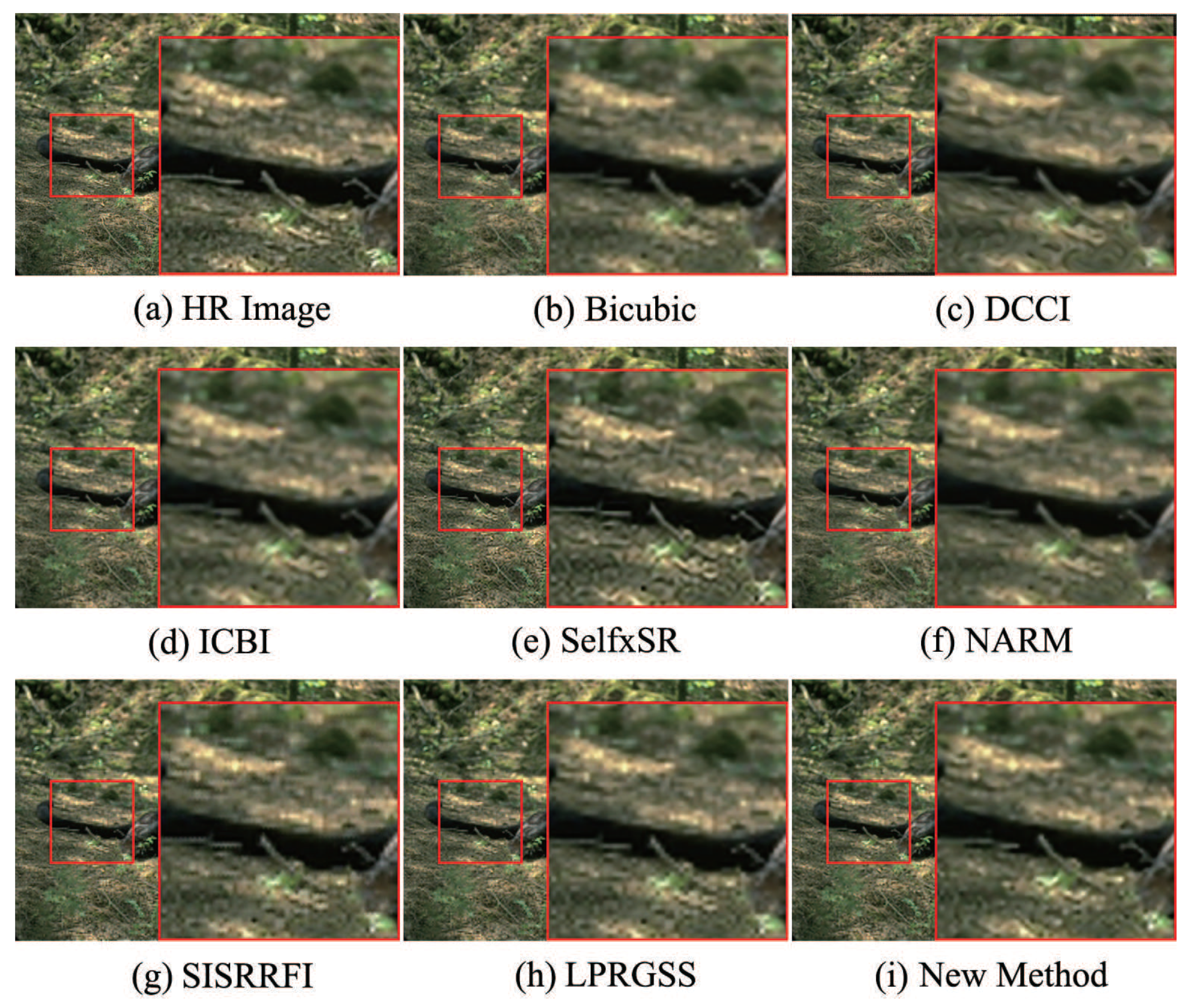
Then, we compare the visual effects of the magnified images. Experiment results show that most of the magnified images by the 8 methods have little difference in visual effects, but there are slight differences in the partially magnified images. The comparison results of visual effect of the 8 methods are given in Figure 4, Figure 5, Figure 6, Figure 7 and Figure 8, where (a) is the HR image and (b), (c), (d), (e), (f), (g), (h), and (i) are magnified images by bicubic, DCCI, ICBI, SelfxSR, NARM, SISRRFI, LPRGSS, and the new method, respectively.
In order to facilitate the comparison of visual effects, we have marked some visually distorted parts on the magnified image, as shown in the red box in Figure 4, Figure 5, Figure 6, Figure 7 and Figure 8. Figure 4 and Figure 5 show the results of the 8 methods for magnifying the two typical grayscale images. In Figure 4, it can be seen that the images (f) and (i) obtained by NARM and new method, respectively, are closest to the HR image (a); the images (c) and (d) obtained by DCCI and ICBI methods are relatively smooth at the edges and producing obvious distortion of lung tissue information; and the images (b), (g), and (h) obtained by the BiCubic, SISRRFI, and LPRGSS, respectively, have sawtooth problems at the edge. In Figure 5, the images (c), (d), and (f) obtained by DCCI, ICBI, and NARM methods, respectively, are relatively smooth at the edges, resulting in reduced detail information. The images (b), (e), (g), and (h) obtained by the bicubic, SelfxSR, SISRRFI, and LPRGSS methods, respectively, have different degrees of sawtooth problems at the edges and the edges are very rough. Overall, the image by the new method (i) is closest to the HR image (a).
Figure 6 and Figure 7 show the results of 8 methods for magnifying two color images in BSD100. For the images in Figure 6, there are small differences between these images, the images (c), (d), and (f) obtained by DCCI, ICBI, and NARM methods, respectively, are relatively smooth, and the texture details of the branches are missing; the images (b), (e), (g) and (h) obtained by the bicubic, SelfxSR, SISRRFI, and LPRGSS methods, respectively, are slightly distorted, such as some details of the branches on the far right side of the tail are missing; and by comparison, the image (i) obtained by the new method is closest to the HR image (a). In Figure 7, the images (c), (d), and (f) obtained by the DCCI, ICBI, and NARM methods, respectively, have shallow wrinkles in the corners of the eye of the elderly and loss of texture on the left side of the eyelids; the image (e) obtained by SelfxSR has the defect of deepening wrinkles in the elderly and does not look real; and in the images (b), (g) and (h) obtained by the bicubic, SISRRFI, and LPRGSS methods, respectively, there are severe jagged edges in the ears and eyelids of the elderly. Overall, the image (i) by the new method is closest to the HR image (a). Figure 8 shows the results of 8 methods for magnifying one aliasing image in AIS. Experimental results show that, for the aliasing images in AIS, the magnified images by the 8 methods have very small visual differences. In Figure 8, relatively speaking, the images (h) and (i) obtained by LPRGSS and the new method are closest to the HR image (a); the images (b), (e), (f), and (g) by bicubic, SelfxSR, NARM, and SISRRFI, respectively, are the second; and the images (c) and (d) by DCCI and ICBI are third. Obviously, in Figure 8, all eight images have the problem of losing details and distortion. Table 2, Figure 8 shows that, for the images in AIS, these 8 methods generally can not get good results; one of the main reasons is that the images obtained by downsampling may destroy the details of the original aliasing image. For example, Figure 9 is the downsampling of the aliasing image (a) in Figure 8, and these two images are obviously different.
5.3. Runtime
We compare the runtime of the 8 methods, and the comparison results are shown in Table 3, where the time unit is seconds. In Table 3, the runtime of the new method is basically the same as the bicubic method. The time in Table 3 of the new method is the time used to magnify the image, but the new method takes 0.207 s to construct the approximation surface. The approximation surface only needs to be constructed once. After the surface is constructed, the image can be magnified by any multiple, and the time taken is basically the same as that of the bicubic method.
5.4. Discussion
The results in Table 1, Table 2 and Table 3 and Figure 4, Figure 5, Figure 6, Figure 7 and Figure 8 show that, among the 8 methods in the comparison, (1) overall, the quality of the magnified images by the new method is the best, followed by LPRGSS method; (2) the bicubic method has the shortest running time, followed by the new method, these two methods are suitable for real-time image magnification; (3) for areas without edges and textures in the image, there is little visual difference between the magnified images by the 8 methods, the 9 images in Figure 6 are examples. In fact, for areas without edges and textures in the image, bicubic method, as the most classical basic image magnification method, can produce the same PSNR and SSIM values as the new method, while for areas with edges and textures in the image, bicubic method generally produces image blocks with poor visual effect. The images (b) in Figure 4, Figure 5, and Figure 7 are examples. The main reason is that the bicubic method constructs each surface patch by passing 16 image pixels, which means that, when bicubic method is used, there is no degree of freedom in constructing bicubic surface; the constructed surface is unique. If the pixels are sampled from different objects, the surface patch constructed by bicubic method will produce larger oscillations, resulting in jagged or blurred pixels at the edges of the image. For magnifying the image without edges and textures, the new method has the advantages of bicubic method. Because the new method uses edge features as constraints to construct quadratic polynomial surface, for magnifying the image with edges and textures, the new method gets better magnified images than bicubic method.
We also tested the images in data sets set5 and set14 and database BSD300. The test results were basically the same as those of the 12 typical images, the images in BSD200, Urban100, and AIS.
6. Conclusions
It is an effective method to construct a surface to approximate the image and then sampling the surface to generate the magnified image, especially when magnifying medical images. The key problem is how to construct the approximation surface. Based on the complexity of image shape, it is an effective strategy to construct local surfaces and to generate a whole sampling surface by the weighted combination of the local surfaces. In this paper, the second-order difference quotient is used to describe the characteristics of the pixels at the edge, which better distinguishes the characteristics difference between the pixels at the edge and the pixels at the non-edge. In the process of local surface construction, we use the edge features of the image as constraints to construct a quadratic polynomial surface patch on the adjacent area of each pixel. Four adjacent quadratic polynomial patches are weighted to form a bicubic surface. All the bicubic surfaces are put together to form the whole sampling surface. The constructed bicubic surface has quadratic polynomial precision. It is inevitable that there are errors in the magnified image obtained from the whole sampling surface. The correction surface can be formed by the approximation error, so as to correct the errors and to improve the approximation accuracy of the whole sampling surface. Due to the use of edge feature constraints to construct local surfaces, each local surface can better maintain the edge features or texture features near the pixels. Experiment results showed that it is an effective method to magnify the image by constructing local surface patches with edge feature constraints, especially for medical image.
Although the magnified image keeps information such as the edge texture of the image well, there is still a lack of edge and texture information. Moreover, the bicubic surface should have bicubic polynomial precision, but the method in this paper has only quadratic polynomial precision. Therefore, our future research work is to improve the retention of edge and texture information and the interpolation accuracy, so that the magnified image has higher image quality and better visual effect.
In addition, Table 2 and Figure 8 show that, for the aliasing images in AIS, the eight methods are not ideal for enlarging the images. It is necessary to study a new image magnification method according to the characteristics of the aliasing images. Because in the aliasing images, there are many edges and the difference of pixel values at the edge is large. One idea to consider is to magnify the aliasing image by the combination of segmentation and fitting. Firstly, the image is segmented, and then, the piecewise fitting patches are constructed based on the segmentation results so as to reduce the oscillation of the patchs as much as possible. This is our second research work we will do next.
Author Contributions
Conceptualization, A.C.; methodology, H.H.; software, L.J.; validation, R.Z.; formal analysis, A.C., H.H., L.J., and R.Z.; investigation, L.J.; resources, H.H.; data curation, R.Z.; writing-original draft preparation, L.J.; writing-review and editing, A.C.; visualization, L.J. and R.Z.; supervision, H.H.; project administration, A.C.; funding acquisition, H.H. All authors have read and agreed to the published version of the manuscript.
Funding
This work is supported by NSFC Joint Fund with Zhejiang Integration of Informatization and Industrialization under Key Project (U1609218) and by the Science and Technology Innovation Program for Distributed Young Talents of Shandong Province Higher Education Institutions under Grant 2019KJN042.
Conflicts of Interest
The authors declare no conflict of interest.
Abbreviations
The following abbreviations are used in this manuscript:
| PSNR | Peak Signal to Noise Ratio |
| SSIM | Structural Similarity |
| HR | Hign Resolution |
| LR | Low Resolution |
| AIS | Aliasing Image Set |
| DCCI | Directional Cubic Convolution Interpolation |
| ICBI | Iterative Curvature-Based Interpolation |
| NARM | Nonlocal Autoregressive Modelin |
| SISRRFI | Single-Image Super-Resolution based on Rational Fractal Interpolation |
| LPRGSS | Low-rank Patch Regularization and Global Structure Sparsity |
References
- Gonzalez, R.C.; Woods, R.E. Digital Image Processing, 2nd ed.; Prentice Hall: Upper Saddle River, NJ, USA, 2002. [Google Scholar]
- Keys, R.G. Cubic convolution interpolation for digital image processing. IEEE Trans. Acoust. Speech Signal Proc. 1981, 29, 1153–1160. [Google Scholar] [CrossRef] [Green Version]
- Park, S.K.; Schowengerdt, R.A. Image reconstruction by parametric cubic convolution. Comput. Vis. Graph Image Proc. 1983, 23, 258–272. [Google Scholar] [CrossRef]
- Munoz, A.; Blu, T.; Unser, M. Least-squares image resizing using finite differences. IEEE Trans. Image Proc. 2001, 10, 1365–1378. [Google Scholar] [CrossRef] [PubMed]
- Zhang, X.; Schowengerdt, X.W. Image interpolation by adaptive 2D autoregressive modeling and soft-decision estimation. IEEE Trans. Image Proc. 2008, 17, 887–896. [Google Scholar] [CrossRef]
- Wu, L.; Liu, Y.; Liu, N.; Zhang, C. High-resolution images based on directional fusion of gradient. Comp. Vis. Media 2016, 2, 31–43. [Google Scholar] [CrossRef] [Green Version]
- Zhou, D.; Shen, X.; Dong, W. Image zooming using directional cubic convolution interpolation. IET Image Proc. 2012, 6, 627–634. [Google Scholar] [CrossRef] [Green Version]
- Giachetti, A.; Asuni, N. Real-time artifact-free image upscaling. IEEE Trans. Image Proc. 2011, 20, 2760–2768. [Google Scholar] [CrossRef]
- Zhang, C.; Zhang, X.; Li, X.; Cheng, F. Cubic surface fitting to image with edges asconstraints. In Proceedings of the 2013 IEEE International Conference on Image Processing, Melbourne, Australia, 15–18 September 2013; pp. 1046–1050. [Google Scholar]
- Zhang, F.; Zhang, X.; Qin, X.; Zhang, C. Enlarging Image by Constrained Least Square Approach with Shape Preserving. J. Comp. Sci. Tech. 2015, 30, 489–498. [Google Scholar] [CrossRef]
- Tang, Y.; Yuan, Y.; Yan, P.; Li, X. Greedy regression in sparse coding space for single-image super-resolution. J. Vis. Commun. Image Represent. 2013, 24, 148–159. [Google Scholar] [CrossRef]
- Yang, J.; Wright, J.; Huang, T.S.; Ma, Y. Image super-resolution via sparse representation. IEEE Trans. Image Process 2010, 19, 2861–2873. [Google Scholar] [CrossRef]
- Dong, W.; Zhang, L.; Lukac, R.; Shi, G. Sparse representation based image interpolation with nonlocal autoregressive modeling. IEEE Trans. Image Proc. 2013, 22, 1382–1394. [Google Scholar] [CrossRef] [PubMed] [Green Version]
- Bevilacqua, M.; Roumy, A.; Guillemot, C.; Morel, M.-L.A. Single-image super-resolution via linear mapping of interpolated self examples. IEEE Trans. Image Process 2014, 23, 5334–5347. [Google Scholar] [CrossRef] [PubMed]
- Huang, J.; Singh, A.; Ahuja, N.; Morel, M.-L.A. Single image super-resolution from transformed self-exemplars. In Proceedings of the 2015 IEEE Conference on Computer Vision and Pattern Recognition (CVPR), Boston, MA, USA, 7–12 June 2015; pp. 5197–5206. [Google Scholar]
- Dong, C.; Loy, C.C.; He, K.; Tang, X. Learning a deep convolutional network for image super-resolution. In ECCV 2014: Computer Vision—ECCV 2014; Springer: Cham, Switzerland, 2014; pp. 184–199. [Google Scholar]
- Dong, C.; Loy, C.C.; He, K.; Tang, X. Image superresolution using deep convolutional networks. IEEE Trans. Pattern Anal. 2016, 38, 295–307. [Google Scholar]
- Ding, N.; Liu, Y.; Fan, L.; Zhang, C. Single image super resolution via dynamic lightweight database with local-feature based interpolation. J. Comp. Sci. Technol. 2019, 34, 537–549. [Google Scholar] [CrossRef]
- Xu, Y.; Quan, Y.; Ling, H.; Ji, H. Dynamic texture classification using dynamic fractal analysis. In Proceedings of the 2011 International Conference on Computer Vision, Barcelona, Spain, 6–13 November 2011; pp. 119–1226. [Google Scholar]
- Liu, M.; Zhao, Y.; Liang, J.; Lin, C.; Bai, H.; Yao, C. Depth map up-sampling with fractal dimension and texture-depth boundary consis tencies. Neurocomputing 2017, 257, 185–192. [Google Scholar] [CrossRef]
- Wee, Y.C.; Shin, H.J. A novel fast fractal super resolution technique. IEEE Trans. Consum. Electron. 2010, 56, 1537–1541. [Google Scholar] [CrossRef]
- Xu, H.; Zhai, G.; Yang, X. Single image super-resolution with detail enhancement based on local fractal analysis of gradient. IEEE Trans. Circuits Syst. Video Technol. 2013, 23, 1740–1754. [Google Scholar] [CrossRef]
- Zhang, Y.; Fan, Q.; Bao, F.; Liu, Y.; Zhang, C. Single-Image Super-Resolution Based on Rational Fractal Interpolation. IEEE Trans. Image Proc. 2013, 22, 3782–3797. [Google Scholar]
- Zhang, M.; Desrosiers, C. High-quality image restoration using low-rank patch regularization and global structure sparsity. IEEE Trans. Image Proc. 2019, 28, 868–879. [Google Scholar] [CrossRef]
- Irani, M.; Peleg, S. Motion analysis for image enhancement: Resolution, occlusion, and transparency. J. Vis. Comm. Image Represent. 1993, 4, 324–335. [Google Scholar] [CrossRef] [Green Version]
- Gan, Z.; Cui, Z.; Chen, C.; Zhu, X. Adaptive joint nonlocal means denoising back projection for image super resolution. In Proceedings of the 2013 IEEE International Conference on Image Processing, Melbourne, Australia, 15–18 September 2013; pp. 630–634. [Google Scholar]
- Zhang, X.; Liu, Q.; Li, X.; Zhou, Y.; Zhang, C. Non-local feature back-projection for image super-resolution. IET Image Proc. 2016, 10, 398–408. [Google Scholar] [CrossRef]
- Wang, H.; Zhang, P.; Zhu, X.; Tsang, I.W.; Chen, L.; Zhang, C.; Wu, X. Incremental subgraph feature selection for graph classification. IEEE Trans. Knowl. Data Eng. 2016, 29, 128–142. [Google Scholar] [CrossRef]
- Wang, H.; Cui, Z.; Chen, Y.; Avidan, M.; Abdallah, A.B.; Kronzer, A. Predicting hospital readmission via cost sensitive deep learning. IEEE/ACM Trans. Comp. Biol. 2018, 15, 1968–1978. [Google Scholar] [CrossRef] [PubMed]
- Kaplan, C.S. Aliasing Artifacts and Accidental Algorithmic Art. In Proceedings of the Renaissance Banff: Bridges 2005: Mathematical Connections in Art, Music and Science, Banff, AB, Canada, 31 July–3 August 2005; pp. 349–356. [Google Scholar]
Figure 1.
A neighborhood of pixels.

Figure 2.
The error image histograms of two groups.

Figure 3.
Twelve typical images, from left to right, from top to bottom: Barbara, Baboon, Boat, Chest, Couple, Crowd, Dollar, Goldhill, Kod, Lake, Lenna, and Peppers.
Figure 3.
Twelve typical images, from left to right, from top to bottom: Barbara, Baboon, Boat, Chest, Couple, Crowd, Dollar, Goldhill, Kod, Lake, Lenna, and Peppers.

Figure 4.
Chest images magnified by eight methods.

Figure 5.
Leena images magnified by eight methods.

Figure 6.
Branch images magnified by eight methods.

Figure 7.
Elderly images magnified by eight methods.

Figure 8.
Aliasing images magnified by eight methods.

Figure 9.
Downsampling of the aliasing image (a) in Figure 8.
Figure 9.
Downsampling of the aliasing image (a) in Figure 8.


Table 1.
Peak Signal-to-Noise Ratio (PSNR) and Structural Similarity (SSIM) values of 12 magnified images by 8 methods.
Table 1.
Peak Signal-to-Noise Ratio (PSNR) and Structural Similarity (SSIM) values of 12 magnified images by 8 methods.
| Image | Bicubic | DCCI | ICBI | SelfExSR | NARM | SISRRFI | LPRGSS | New | ||||||||
|---|---|---|---|---|---|---|---|---|---|---|---|---|---|---|---|---|
| PSNR | SSIM | PSNR | SSIM | PSNR | SSIM | PSNR | SSIM | PSNR | SSIM | PSNR | SSIM | PSNR | SSIM | PSNR | SSIM | |
| Baboon | 23.99 | 0.731 | 22.76 | 0.659 | 22.73 | 0.666 | 23.70 | 0.763 | 22.87 | 0.663 | 23.67 | 0.731 | 24.28 | 0.767 | 24.32 | 0.772 |
| Barbara | 25.43 | 0.794 | 24.10 | 0.742 | 23.94 | 0.743 | 24.42 | 0.806 | 24.12 | 0.744 | 24.78 | 0.787 | 25.66 | 0.819 | 25.15 | 0.812 |
| Boat | 32.28 | 0.917 | 29.42 | 0.879 | 29.42 | 0.882 | 32.66 | 0.928 | 29.52 | 0.879 | 32.95 | 0.903 | 32.72 | 0.926 | 33.13 | 0.930 |
| Chest | 29.56 | 0.920 | 26.23 | 0.861 | 26.23 | 0.876 | 31.53 | 0.940 | 26.32 | 0.786 | 30.33 | 0.928 | 30.38 | 0.936 | 31.57 | 0.941 |
| Couple | 29.66 | 0.860 | 27.50 | 0.807 | 27.47 | 0.810 | 29.94 | 0.872 | 27.61 | 0.805 | 28.82 | 0.843 | 30.04 | 0.876 | 30.33 | 0.880 |
| Crowd | 32.82 | 0.945 | 28.64 | 0.896 | 28.77 | 0.902 | 34.03 | 0.957 | 28.74 | 0.894 | 32.39 | 0.928 | 33.51 | 0.954 | 34.35 | 0.960 |
| Dollar | 20.42 | 0.670 | 19.41 | 0.623 | 19.30 | 0.622 | 20.31 | 0.694 | 19.51 | 0.629 | 20.61 | 0.675 | 20.62 | 0.698 | 20.69 | 0.701 |
| Goldhill | 31.34 | 0.860 | 29.20 | 0.810 | 29.25 | 0.815 | 31.28 | 0.869 | 29.24 | 0.804 | 30.96 | 0.858 | 31.68 | 0.875 | 31.82 | 0.878 |
| Kod | 26.51 | 0.861 | 24.73 | 0.822 | 24.49 | 0.822 | 26.90 | 0.881 | 24.88 | 0.826 | 26.86 | 0.855 | 26.91 | 0.879 | 27.22 | 0.884 |
| Lake | 30.62 | 0.872 | 27.54 | 0.825 | 27.76 | 0.834 | 31.05 | 0.880 | 27.78 | 0.826 | 30.41 | 0.867 | 31.10 | 0.884 | 31.39 | 0.886 |
| Lenna | 32.25 | 0.942 | 29.16 | 0.903 | 29.16 | 0.908 | 33.21 | 0.950 | 29.24 | 0.900 | 31.95 | 0.940 | 32.79 | 0.951 | 33.56 | 0.955 |
| Peppers | 33.76 | 0.890 | 30.73 | 0.863 | 30.73 | 0.865 | 34.74 | 0.893 | 30.79 | 0.859 | 32.76 | 0.888 | 34.18 | 0.898 | 34.69 | 0.899 |
| Average | 29.05 | 0.855 | 26.62 | 0.807 | 26.61 | 0.812 | 29.48 | 0.869 | 26.72 | 0.801 | 28.87 | 0.850 | 29.49 | 0.872 | 29.85 | 0.875 |
Table 2.
Average PSNR and SSIM values for 8 methods for BSD100, Urban100, and aliasing image set (AIS).
Table 2.
Average PSNR and SSIM values for 8 methods for BSD100, Urban100, and aliasing image set (AIS).
| Image | Bicubic | DCCI | ICBI | SelfExSR | NARM | SISRRFI | LPRGSS | New | |
|---|---|---|---|---|---|---|---|---|---|
| BSD100 | PSNR | 29.73 | 27.71 | 27.76 | 30.10 | 27.84 | 30.03 | 30.13 | 30.48 |
| SSIM | 0.853 | 0.800 | 0.807 | 0.871 | 0.798 | 0.864 | 0.871 | 0.875 | |
| UrBan100 | PSNR | 26.75 | 24.79 | 24.72 | 27.64 | 25.02 | 26.86 | 27.18 | 27.77 |
| SSIM | 0.848 | 0.795 | 0.796 | 0.878 | 0.803 | 0.856 | 0.868 | 0.880 | |
| AIS | PSNR | 9.07 | 8.64 | 8.49 | 8.70 | 8.59 | 8.65 | 9.12 | 9.13 |
| SSIM | 0.269 | 0.208 | 0.206 | 0.332 | 0.219 | 0.195 | 0.320 | 0.318 | |
Table 3.
Runtime of 12 images with 8 methods (Unit: seconds).
| Image | Bicubic | DCCI | ICBI | SelfExSR | NARM | SISRRFI | LPRGSS | New |
|---|---|---|---|---|---|---|---|---|
| Barbara | 0.018 | 1.849 | 5.297 | 183.453 | 332.389 | 320.068 | 176.514 | 0.020 |
| Baboon | 0.018 | 1.614 | 5.000 | 170.285 | 351.381 | 318.440 | 180.015 | 0.020 |
| Boat | 0.018 | 1.633 | 3.922 | 176.946 | 335.560 | 317.841 | 175.639 | 0.020 |
| Chest | 0.018 | 1.623 | 5.548 | 189.318 | 394.686 | 317.895 | 161.575 | 0.020 |
| Couple | 0.018 | 1.679 | 5.188 | 181.168 | 343.976 | 318.039 | 174.233 | 0.020 |
| Crowd | 0.018 | 1.857 | 5.389 | 171.767 | 463.896 | 330.901 | 174.872 | 0.020 |
| Dollar | 0.018 | 1.621 | 4.676 | 185.658 | 405.255 | 326.665 | 178.925 | 0.020 |
| Goldhill | 0.018 | 1.617 | 4.391 | 174.468 | 405.280 | 325.677 | 176.006 | 0.020 |
| Kod | 0.018 | 1.611 | 3.410 | 181.206 | 401.058 | 328.210 | 173.926 | 0.020 |
| Lake | 0.018 | 1.669 | 4.490 | 175.183 | 392.478 | 330.892 | 175.263 | 0.020 |
| Lenna | 0.018 | 1.578 | 4.960 | 173.818 | 347.464 | 340.423 | 173.287 | 0.020 |
| Peppers | 0.018 | 1.584 | 4.151 | 171.785 | 343.719 | 334.731 | 173.759 | 0.020 |
| Average | 0.018 | 1.849 | 5.297 | 183.453 | 332.389 | 320.068 | 174.501 | 0.020 |
© 2020 by the authors. Licensee MDPI, Basel, Switzerland. This article is an open access article distributed under the terms and conditions of the Creative Commons Attribution (CC BY) license (http://creativecommons.org/licenses/by/4.0/).
Share and Cite
MDPI and ACS Style
Ji, L.; Zhang, R.; Han, H.; Chaddad, A. Image Magnification Based on Bicubic Approximation with Edge as Constraint. Appl. Sci. 2020, 10, 1865. https://doi.org/10.3390/app10051865
AMA Style
Ji L, Zhang R, Han H, Chaddad A. Image Magnification Based on Bicubic Approximation with Edge as Constraint. Applied Sciences. 2020; 10(5):1865. https://doi.org/10.3390/app10051865
Chicago/Turabian StyleJi, Linlin, Rui Zhang, Huijian Han, and Ahmad Chaddad. 2020. "Image Magnification Based on Bicubic Approximation with Edge as Constraint" Applied Sciences 10, no. 5: 1865. https://doi.org/10.3390/app10051865
Note that from the first issue of 2016, this journal uses article numbers instead of page numbers. See further details here.