Region-Based CNN Method with Deformable Modules for Visually Classifying Concrete Cracks


1
Key Laboratory for Damage Diagnosis of Engineering Structures of Hunan Province, Hunan University, Changsha 410082, China
2
College of Civil Engineering, Hunan University, Changsha 410082, China
*
Author to whom correspondence should be addressed.
Appl. Sci. 2020, 10(7), 2528; https://doi.org/10.3390/app10072528
Submission received: 2 March 2020
/
Revised: 28 March 2020
/
Accepted: 2 April 2020
/
Published: 7 April 2020
(This article belongs to the Special Issue Health Structure Monitoring for Concrete Materials, Volume II)
Abstract
:Cracks are often the most intuitive indicators for assessing the condition of in-service structures. Intelligent detection methods based on regular convolutional neural networks (CNNs) have been widely applied to the field of crack detection in recently years; however, these methods exhibit unsatisfying performance on the detection of out-of-plane cracks. To overcome this drawback, a new type of region-based CNN (R-CNN) crack detector with deformable modules is proposed in the present study. The core idea of the method is to replace the traditional regular convolution and pooling operation with a deformable convolution operation and a deformable pooling operation. The idea is implemented on three different regular detectors, namely the Faster R-CNN, region-based fully convolutional networks (R-FCN), and feature pyramid network (FPN)-based Faster R-CNN. To examine the advantages of the proposed method, the results obtained from the proposed detector and corresponding regular detectors are compared. The results show that the addition of deformable modules improves the mean average precisions (mAPs) achieved by the Faster R-CNN, R-FCN, and FPN-based Faster R-CNN for crack detection. More importantly, adding deformable modules enables these detectors to detect the out-of-plane cracks that are difficult for regular detectors to detect.
1. Introduction
In the field of structural condition assessment, cracks are usually the most intuitive and relatively reliable indicator for evaluating the performance of a structure [1]. Based on audiovisual methods, stress-wave methods, and electromagnetic methods, plenty of research on the detection of structural cracks has been carried out [2,3]. Currently, the main methods can be divided into two categories: one type based on acoustic waves [4] and the other type based on image analysis [5]. As early as the 1990s, the acoustic emission (AE) technology was gradually promoted and used to test the integrity of concrete structures in Japan, although it was not always successful when applied to practical problems. With the development of testing equipment, Ohno and Ohtsu [6] classified crack patterns in concrete by the AE technology. On this basis, Aggelis [7] conducted an experiment to monitor several types of concrete crack during bending, and further proposed and clarified some AE indicators that can classify the crack mode under different stress states. Farhidzadeh et al. [8] proposed a new probabilistic method based on the AE Gaussian mixture model (GMM) that can more efficiently classify the crack patterns in reinforced concrete structures. Aldahdooh and Bunnori [9] also adopted the AE signals to classify crack types of reinforced concrete beams subjected to four-point bending. Over the past years, portable AE equipment has been applied to monitor the cracks in prefabricated prestressed concrete beams during construction [10]. As an effective method for classification of structural cracks, the AE method has high demand on equipment and is seriously affected by noise. Unlike the AE method, the image analysis method uses images of the structure surface to identify structural cracks. During the past decades, traditional vision inspection has been developed from naked-eye inspection to the machine-vision inspection. Currently, naked-eye inspection is still the most common method used to identify structural cracks. However, this method is often time-consuming and subjective, and can be dangerous in some circumstances. To tackle these issues, many studies have been conducted on automatic detection of cracks based on the machine vision technology. In these researches, many image-processing algorithms, including mathematical morphology [11], digital image correlation (DIC) [12,13], image binarization [14], percolation model [15], wavelet transforms [16], and edge detectors [17] have been developed to detect cracks in obtained images. Combined with drone technology in civil engineering, the detection of cracks has become more convenient and safer [18,19,20]. However, the performance of these methods is susceptible to environmental conditions such as the light conditions. Among the above methods, DIC technology, as a relatively new nondestructive and noncontact full field displacement measuring technique, has been widely applied to the study of concrete fracture [21]. The classical DIC method classifies cracks by comparing the pixel features of the point of interest at different states to those at the initial state [21,22], which is less affected by environmental noise. However, compared with the intelligent detection method, it still needs to judge the position of the crack artificially before the detection, and its effectiveness is limited by the uncertainty of the constitutive parameters and boundary conditions [23].
In the early 1990s, neural networks were widely applied to crack detection, and one of the most popular multilayer neural networks has been the convolutional neural network (CNN), which is able to recognize crack patterns from images with minimal preprocessing. During the past decade, with the improvement of computing power of high-performance graphics processing unit (GPU), the performance of the CNN has been improved significantly. Cha et al. [24] used a CNN to identify cracks in concrete structures, and it was found that the proposed method was superior to the traditional Canny and Sobel edge detection algorithms in applicability, convenience, and detection accuracy. Kim et al. [25] presented a CNN-based method to identify concrete cracks, which performed well on detecting the crack and noncrack images under noisy conditions, where it is difficult for traditional image-processing algorithms to identify cracks. Cha et al. [26] proposed a structural damage detector based on the Faster R-CNN for detecting multitype damages including cracks. Xu et al. [27] proposed a concrete crack detection method with a novel CNN architecture, which improved detection accuracy without pretraining. Dung and Anh [28] proposed a deep fully convolutional network (FCN)-based crack detection method to detect cracks and assess crack density and achieved satisfactory performance. Recently, a new deep learning architecture based on CNN to perform real-time pixel-level segmentation of cracks was proposed by Choi and Cha [29], which improves the sensitivity of crack detectors. However, as the convolutional layer and pooling layer of the regular CNN both lack the internal mechanism to deal with out-of-plane deformation [30,31], the detection accuracy for the out-of-plane cracks is often very low [32].
In the present study, a region-based concrete crack detector with deformable modules is proposed to achieve better identification of out-of-plane cracks. Three different types of region-based detectors (namely, the Faster R-CNN, R-FCN, and FPN-based Faster R-CNN) with and without deformable modules are introduced and used to detect three common cracks, including transverse crack, longitudinal crack, and alligator crack [33,34]. The superiority of adding deformable modules is proved through comparative analysis.
2. Methodology
The schematic diagram of the proposed method is shown in Figure 1. In the first stage, three regular region-based object detection networks (Faster R-CNN, R-FCN, and FPN-based Faster R-CNN) under the framework of the deep residual network (ResNet-101) are introduced, based on which three new networks are established by adding deformable modules to each of these networks. In the second stage, procedures to build databases are described. In the last stage, the implementation details are introduced and the superiority of the proposed method is proved.
2.1. Selection of CNN Backbone
The CNN is used to implement feature extraction from images. Usually, a CNN can extract more features from images if it has more layers. Since the birth of the AlexNet, CNN architecture has become deeper and deeper. For instance, the AlexNet only has five convolution layers, while the numbers of layers of the VGGNet and GoogleNet have been increased to 19 and 22, respectively. However, the model tends to become unstable if only the depth of the network increases as gradient vanishing and explosion may occur and result in nonconvergence during the model training process [35,36]. To overcome the bottleneck, He et al. [37] proposed a residual network (ResNet) composed of a batch of regularized residual blocks which contain an architecture known as “shortcut connection”. With the help of the “shortcut connection” and batch normalization during the model training process, data transmission can skip some intermediate layers, which not only helps accelerate convergence but also prevents overfitting. Currently, there are five common structures for the residual network, including ResNet-18, ResNet-34, ResNet-50, ResNet-101, and ResNet-152. As shown in Figure 2, the residual network is mainly composed of different types of residual blocks that are called building blocks or bottlenecks. In the present study, to make a good balance between the computation cost and detection accuracy, ResNet-101 was selected for the CNN architecture to extract image features.
2.2. Region-Based Object Detection Framework
The overall architectures of the three adopted region-based object detection networks, including the Faster R-CNN, R-FCN, and FPN-based Faster R-CNN, are shown in Figure 3.
As one of the most widely used object detection networks in recent years, Faster R-CNN greatly improves detection accuracy and computational efficiency compared with the original R-CNN object detection network. Based on the main architecture of Faster R-CNN, the R-FCN was developed with position-sensitive region of interest (RoI) pooling and can double the detection speed by developing optimizing algorithm for sharing parameters. The introduction of FPN solves the contradiction between the resolution and the semantic information of characteristic images with different depths, and improves the detection ability of the model for small objects. The details of the three networks are explained briefly as follows.
2.2.1. Faster R-CNN (Region-Based Convolutional Neural Networks)
Resnet-101 based Faster R-CNN uses 91 layers from conv1-x to conv4-x as shared convolutional layers to extract image features at the beginning, and then bifurcates into two parts from the output of conv4-x as shown in Figure 3a. One part is the region proposal network (RPN) for region proposals, and the other is directly connected with a RoI Pooling layer. Each region proposal from the RPN is input into the RoI Pooling layer and mapped to a feature of 7 × 7. Then all outputs are fed into the conv5-x that acts as the original full connection layer. Finally, for each of the K anchors of each object detected in the input image, two scores and four coordinates will be output, respectively, through the classification layer and regression layer.
2.2.2. R-FCN (Region-Based Fully Convolutional Network)
The overall architecture of the R-FCN is similar to that of the Faster R-CNN, in which the RPN network is adopted for region proposal generation. Unlike the conventional R-CNN, the fully connected (FC) layer after the RoI pooling layer is removed, and the original RoI pooling layer is replaced by a so-called position-sensitive RoI pooling layer to integrate the location information into the network and thus improve computational efficiency. As can be seen from Figure 4, a feature map is followed by a position-sensitive score map, and nine sub-regions of the position-sensitive score map correspond to nine different positions of an object, which will be further used as the score mapping of each position to finally determine whether the object is contained. The process of score mapping of each position, known as the average voting, is a quite simple calculation for preliminary classification, which gives the detector not only high computing efficiency but also good detection accuracy.
2.2.3. FPN (Feature Pyramid Network)-Based Faster R-CNN
Feature pyramid network combines the upper layer (used to acquire low-resolution but strong semantical features) and the lower layer (used to acquire high-resolution but weak semantical features) through lateral connections to improve the capability of feature extraction. Because of this, the FPN helps solve the multiscale detection problem. In practice, the sizes of cracks in civil structures are completely random. Therefore, adding the FPN algorithm to the detector can theoretically improve the accuracy of crack detection. The part that combines the FPN and the Faster R-CNN is shown in Figure 5. Specifically, the feature pyramid architecture is composed of five feature maps denoted as {P2, P3, P4, P5, P6}, among which P2, P3, P4, and P5 are calculated by feature maps C2, C3, C4, and C5 with the lateral connection, respectively, and P6 is generated by the max pooling operation of P5. More details about the combination of the FPN and Faster R-CNN can be found in the study of [38].
2.3. Combination of Deformable Operation Module
In this section, a deformable convolution module and deformable RoI pooling module are introduced and embedded into the three detectors discussed previously to enhance their ability for crack detection. The basic idea of deformable modules is to replace the original fixed-position sampling matrix with the deformable sampling matrix whose structure can be determined by a convolution algorithm that calculates the offset of the sampling position. Corresponding to different detection networks, there are three different deformable modules used in this study.
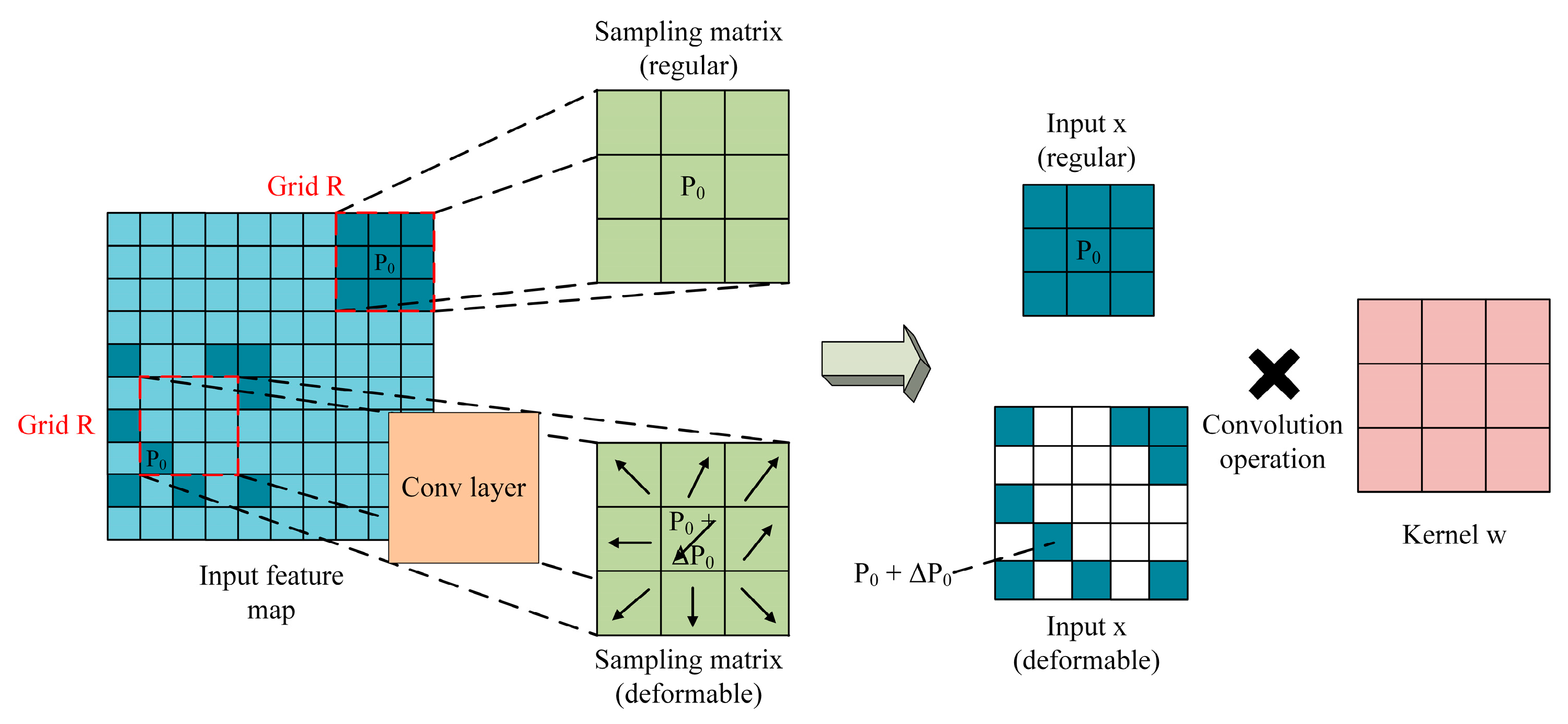
2.3.1. Deformable Convolution
Figure 6 shows the difference between the regular convolution and the deformable convolution. From Figure 6, it can be seen that the main difference of the two convolutions is that the sampling matrix of the former is fixed and regular while that of the latter is unfixed and deformable. Therefore, the receptive field used to conduct dot product with the kernel is regular for the former and is irregular for the latter. It should be noted that the offset of the sampling matrix of the deformable convolution is determined based on the algorithm that can better learn the geometrical property of the objects to be detected, and all the results of three detectors are based on using deformable convolution in the last three convolutional layers (i.e., the 3 × 3 filter in Conv5_x) in the ResNet-101 feature extraction network.
2.3.2. Deformable RoI Pooling
A regular RoI pooling transforms a rectangular region proposal into a feature with fixed size. As shown in Figure 7, the output of the regular RoI pooling can be obtained through (1).
In the deformable RoI pooling, as can be seen from Figure 8, firstly, at the top path, the feature map is generated through the regular RoI pooling; after that, a FC layer generates the normalized offsets that is then converted to the offset through (2), where γ = 0.1. The offset normalization is indispensable to ensure that the offset learning is not affected by the RoI size.
Finally, at the bottom path, the deformable RoI pooling is conducted and the output feature map is pooled based on regions with augmented offsets through (3):
2.3.3. Deformable Position-Sensitive (PS) RoI Pooling
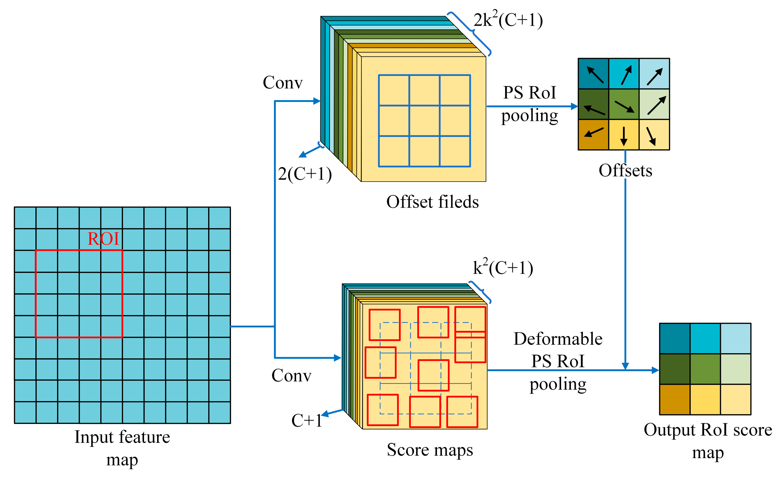
For original PS RoI pooling in R-FCN, all the input feature maps are firstly converted to k2 score maps for each object class as mentioned before (In total C + 1 for C object classes + 1 background). In deformable PS RoI pooling, as shown in Figure 9, at the top path, similar to the original one, convolution is firstly used to generate 2k2(C + 1) score maps. That means, for each class, there will be k2 score maps. These k2 score maps represent the {top-left (TL), top-center (TC), …, bottom right (BR)} of the object whose offsets are desired to learn. The original PS RoI pooling for the offset (top path) is done in the sense that they are pooled with the same area and the same color in Figure 9. Finally, at the bottom path, deformable PS RoI pooling is implemented to pool the feature maps augmented by the offsets obtained from the top path.
3. Implementation
In this section, the establishment of crack databases, the configuration of workstation, and the evaluation indexes for the models are introduced briefly.
3.1. Building the Database
Preparing database in advance is necessary for training, validating, and testing the model. Since 2012, many image databases have been built, such as ImageNet, CIFAR, MNIST, Pascal VOC, COCO common objects data set, OpenImage, etc., which contain a large number of labeled images of common objects. In recent years, some image databases for civil structures have also been established [39,40,41]. However, the crack images in these databases are often used for training binary classification models, which means that data types are only classified into two categories of positive samples and negative samples. Up to now, the public database which contains several types of labeled cracks has not been established yet.
In order to achieve multitype crack detection, images of three common types of cracks are collected [33,34], including the alligator crack, the longitudinal crack, and the transverse crack, as shown in Figure 1. These crack images were obtained from two ways, including shooting on site and searching from the internet. The number of crack images obtained from the former method is 200, and these images were collected from five representative concrete bridges with different ages using the Canon 77D camera with a resolution of 5400 × 4800. The second group of images comes from Baidu image recognition (https://graph.baidu.com/pcpage/index?tpl_from=pc), which has the function of searching similar images. By inputting concrete crack images obtained from the first method into the Baidu engine, the web page can provide similar images. Six-hundred-and-forty qualified images of the three types of cracks provided by Baidu image recognition were selected manually. These images were actually captured in different natural environments and shooting conditions and some contained out-of-plane crack images. In total, 840 crack images with different pixel sizes were obtained. In order to reduce the computational cost, the sizes of all these obtained images were adjusted to 227 × 227 pixels through image processing. In addition, through data augmentation (horizontal flip and mirror), 1860 JPG images (620 alligator, 620 longitudinal, 620 transverse) with 227 × 227 pixels were finally obtained for database preparation. These images were labeled manually with the open-source image annotation program (label-Img). It should be noted that if there are two or more cracks in an image, all cracks in the image were labeled and saved in one XML file instead of extracting and marking each damage individually as Kim et al. [42] did. The number of images used for testing accounts for 20% of the total dataset, which is randomly selected and manually screened.
3.2. Workstation and Training Settings
The equipment used for calculation in the study is a desktop workstation with CUDA 10.0, cudnn 7.1, and MXnet deep learning framework installed on the Ubuntu 16.04 system. The hardware configuration of the workstation is as follows: a Core i7-9400Fk @2.9 GHz CPU, 16GB DDR4 memory, and a colorful GeForce RTX 2080 ti graphics processing unit (GPU) with 11 GB memory.
Determining the hyper-parameters is necessary to train a deep learning model. Previous studies have proven that three key parameters, including the anchor size, batch size, and learning rate, have a significant impact on the performance of a deep learning model [43]. In the present study, two groups of anchor sizes (8, 16, 32 and 32, 64, 128), two batch sizes (64, 256), and three learning rates (0.001, 0.0001, and 0.0005) were adopted to train these models under consideration. Therefore, there are 12 combinations of these parameters for each model training. Each case was trained by an end-to-end training strategy. During the training process, the average loss for every 100 batches was recorded and the model for each training epoch was saved. It should be noted that if the crack area matches the crack type of the ground truth with the intersection over union (IoU) at least 50% and the calculated probability of softmax greater than 0.7, the area is counted as a true positive.
3.3. Evaluation Index
The loss, which can be considered as the error between the predicted result and the true result, is a vital index to judge whether convergence is achieved during the training process. Four loss functions were adopted during the model training process, namely, the RPNLogLoss, RCNNLogLoss, RPNL1Loss, and RCNNL1Loss. The RPNLogLoss is used to calculate the classification loss for the RPN network and is expressed as follows:
where is the predicted probability of being an object in the ith anchor, and is 0 or 1 for the negative label and positive label, respectively.
RCNNLogLoss is used to calculate the classification loss of the detection network, which can be calculated as:
where and are the predicted class scores and true class scores, respectively.
RPNL1Loss is used to calculate the regression loss of the RPN network, which can be expressed as:
where is a vector with four parameters determining the sizes and the position of the predicted bounding box, and is also a vector with four parameters determining the sizes and the position of the ground truth.
RCNNL1Loss is used to calculate the regression loss of the detection network, which can be expressed by:
where and also represent the coordinates and the sizes of the ground truth box and predicted bounding box, respectively, and the smooth function in (7) and (8) are both defined as:
The average precision (AP) is used to evaluate the detection accuracy of each category and the mean average precision (mAP) is the average of the APs of all categories under consideration. Details about calculating the APs and mAP can be found in PASCAL VOC Challenge 2007 [44].
4. Discussions and Comparative Study of the Testing Results
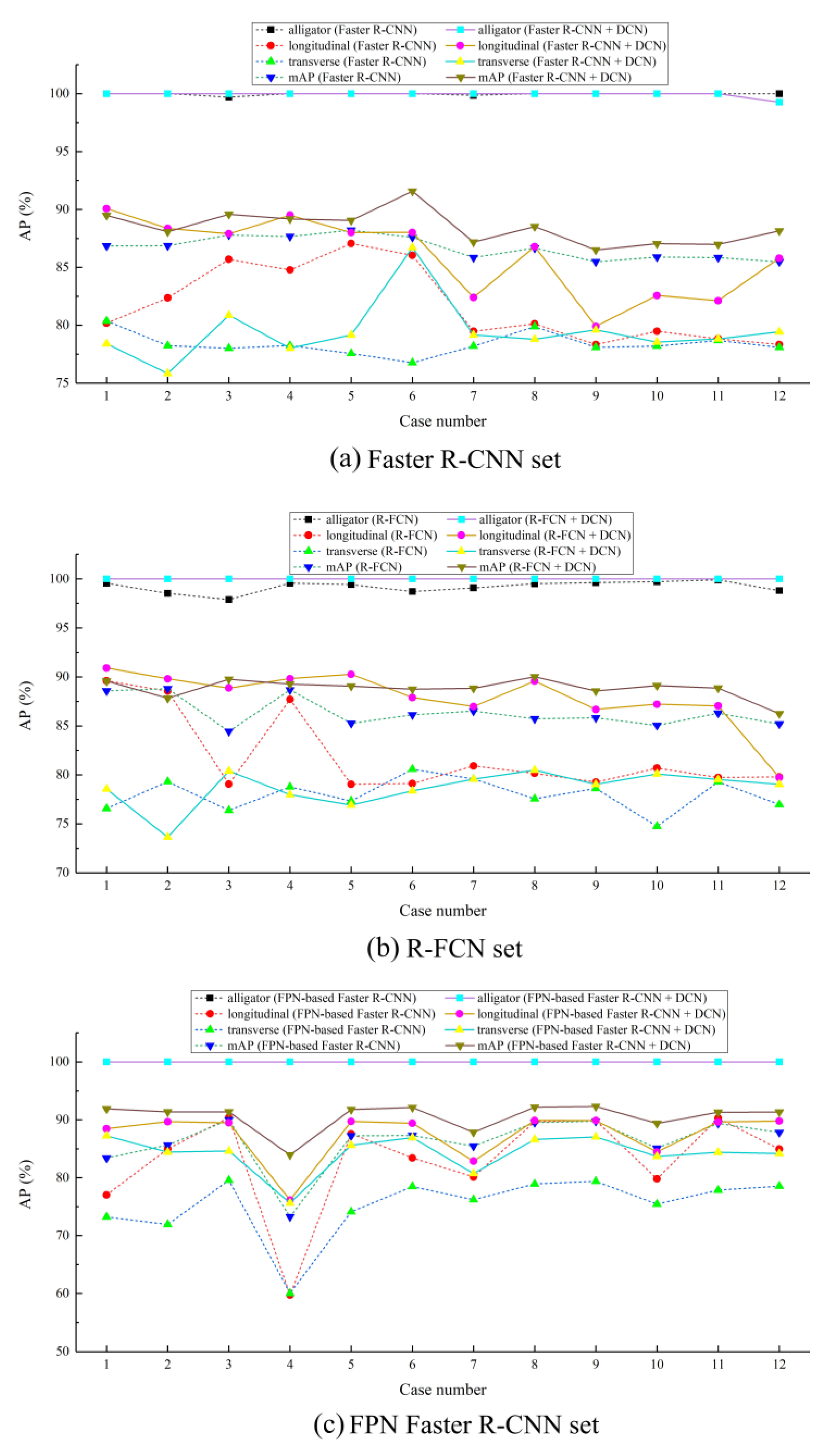
The APs and mAPs of 12 cases for each of the six detectors (three regular and three deformable detectors) trained for 50 epochs are demonstrated in Table 1, Table 2 and Table 3, and in Figure 10. In general, the testing results prove that adding deformable modules can improve the detection accuracy. The optimal combination of parameters for each detector is found through a trial-and-error process.
4.1. Training Results Based on Faster R-CNN
Training the original Faster R-CNN occupies 4 GB of graphics memory, and after adding deformable modules, the graphics memory required rises to 6 GB. Figure 11a,d show the variation of training loss against the number of epochs of Case 6, from which it can be found that almost all training losses fall rapidly at the beginning, and gradually stabilize after training for 50 epochs. Therefore, all the experiments in the study were conducted for 50 epochs, and the time required for each training of the model with and without deformable modules is 8 h and 6 h, respectively. It can be seen from Figure 10a that the APs of the detector with deformable modules is higher than that without deformable modules by different degrees, and the variation of accuracy improvement is between 0% and 9.94%. Specifically, the detector with deformable modules in Case 6 achieves a detection accuracy of 100%, 88.03%, and 86.71% for the alligator crack, longitudinal crack, and transverse crack, respectively, and the mAP is increased by 3.98% compared with the original detector without deformable modules.
4.2. Training Results Based on R-FCN
Training the original R-FCN occupies 4 GB of graphics memory, and after adding deformable modules the graphics memory required raises to 6 GB. Figure 11b,e show that almost all training losses in Case 8 fall rapidly at the beginning, and gradually stabilize after training for 50 epochs, which is basically the same as that of Faster R-CNN. The time required for each training of the model with and without deformable modules is 9 h and 7.5 h, respectively. It can be seen from Figure 10b that the APs of the detector with deformable modules is higher than that without deformable modules, and the improvement of detection accuracy is more obvious compared with that of the Faster R-CNN. Specifically, the detector with deformable modules in Case 8 achieves a detection accuracy of 100%, 89.57%, and 80.48% for the alligator crack, longitudinal crack, and transverse crack, respectively, and mAP is increased by 4.28% compared to the original detector without deformable modules.
4.3. Training Results Based on FPN-Based Faster R-CNN
Training the original FPN-based Faster R-CNN occupies 8 GB of graphics memory, and after adding deformable modules the graphics memory required rises to 11 GB. As shown in Figure 11c,f, the losses in Case 6 also showed the same trend as the previous cases discussed. The time required for each training of the model with and without deformable modules is 7.5 h and 6 h, respectively. It can be seen from Figure 10c that the AP of the detector with deformable modules is higher than that without deformable modules, and the variation of accuracy improvement is between 0% and 16.43%. Specifically, the detector with deformable modules in Case 6 achieves a detection accuracy of 100%, 89.41%, and 86.93% for the alligator crack, longitudinal crack, and transverse crack, respectively, and the mAP is increased by 4.81% compared to the original detector without deformable modules.
4.4. Analysis and Discussion of the Testing Results
Based on the discussion above, it can be seen that for all the three types of cracks under consideration, the detection accuracy of all the three detectors with deformable modules is improved compared to that of the corresponding detectors without deformable modules. The accuracy improvement for different cracks is different, with 4% to 8% improvement for longitudinal and transverse cracks and less than 1% improvement for alligator cracks. The reason why the accuracy improvement for the alligator crack is not obvious is that the detection accuracy of all the detectors without deformable modules is already very high (almost 100%). There may be two explanations for the high detection accuracy of the alligator crack: (1) the characteristics of the longitudinal and transverse crack are quite different from that of the alligator crack; and (2) the features of alligator cracks account for a large part of the image, which makes the object annotation more obvious. In addition, it is found that the learning rate and anchor size are quite important hype-parameters for training the model, while the batch size has little effect on the detection accuracy.
It can be seen from Table 1, Table 2 and Table 3 that the Faster R-CNN, the R-FCN, and the FPN-based Faster R-CNN achieved a relatively better performance in Case 6, Case 8, and Case 6, respectively, and the mAP of the three detectors with deformable modules is 91.58%, 90.01%, and 92.11%, respectively. Figure 12 shows the variation of mAPs with the number of epochs of the detectors in their optimal cases, from which it can be seen that the overall detection accuracy of the three detectors increases sharply in the early stage of training, and gradually become stable after 50 epochs. With deformable modules, all three original detectors achieved better detection accuracy and the FPN-based Faster R-CNN achieved the highest detection accuracy due to the idea of multiscale detection.
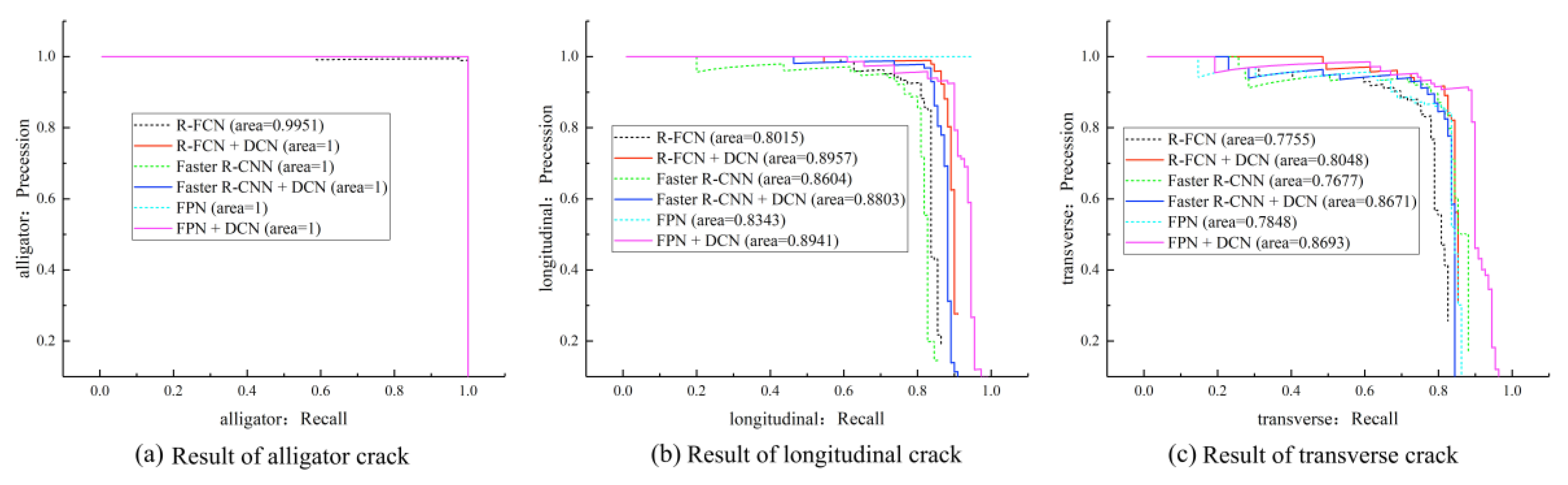
The precision-recall (PR) curves of the detectors in their optimal cases are drawn in Figure 13, from which it can be seen that with the improvement of recall, the precision of training model can still be maintained at a high level, which is particularly significant for detecting cracks in civil structures.
The visualization of some testing results obtained from the optimal cases mentioned above are shown in Figure 14. During the visualization process, the threshold score of the anchor and the threshold value of non-maximum suppression were adopted as 0.8 and 0.3, respectively. It can be seen from Figure 14 that the cracks captured under different shooting environments were accurately detected although several missed detections occurred. It should be noted that the detection accuracy of the detectors for detecting the longitudinal and transverse cracks can be further improved by augmenting the database.
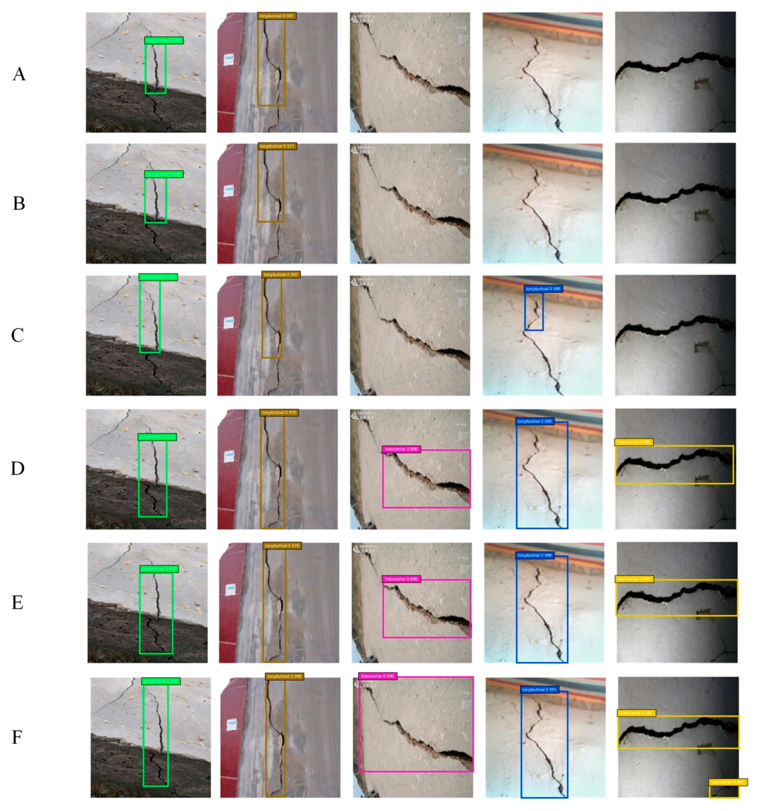
5. Performance on Detecting Cracks with Out-of-Plane Deformation
To better illustrate the advantages of the deformable modules, five new images were captured and classified with the six detectors under the optimal configurations, and the results are shown in Figure 15. In each row in Figure 15, from left to right, the crack in the first image was taken for the corner of a concrete structure, the cracks in the third and fifth images were taken for the surface of concrete piers with oval cross sections, and the cracks in the second and fourth images were taken for two flat concrete structures. Therefore, the cracks in the first, third, and fifth images can be regarded as out-of-plane cracks and the cracks in the other two images can be regarded as in-plane cracks. From Figure 15, it can be seen that for the detectors without a deformable module, the cracks in the first and second images are partially identified while the cracks in the other three images are barely classified successfully. However, for the detectors with deformable modules, the cracks in all five images were almost classified completely accurately. This indicates that adding deformable modules helps these detectors classify not only in-plane cracks but out-of-plane cracks.
6. Conclusions
In the present study, a new idea of embedding deformable modules into traditional region-based crack detectors was proposed. The new crack detector not only improves the precision of crack detection, but also enables the detection of out-of-plane cracks that are difficult for traditional crack detectors to detect. Three networks, including the Faster R-CNN, R-FCN, and FPN-based Faster R-CNN, were adopted to demonstrate the feasibility and efficacy of the new crack detector. A total 1860 images, with uniform size of 227 × 227 pixels, of three types of cracks (alligator, longitudinal, and transverse) were obtained and used as the dataset. Thirty-six cases were investigated by using the three detectors with and without deformable modules. The testing results show that with the addition of deformable modules the mAPs of the Faster R-CNN, R-FCN, and FPN-based Faster R-CNN were improved by 1.76%, 2.44%, and 4.41%, respectively. Specifically, under the optimal configuration, the mAPs of the three detectors with deformable modules were increased by 3.98%, 4.28%, and 4.81%, respectively, compared to that of the three detectors without deformable modules. More importantly, embedding deformable modules enables the three detectors to detect out-of-plane cracks in concrete. Due to the multi-scale feature extraction of FPN, the FPN-based Faster R-CNN showed the best performance among the three detectors, achieving the highest mAP of 92.11% and APs of 100%, 89.41%, and 86.93% for alligator, longitudinal, and transverse cracks, respectively.
Although deformable modules have proven to improve the detection accuracy of in-plane and out-of-plane cracks, at this stage it only works for surface-breaking cracks and still has difficulty to detect crack depth. In the future, efforts will be made to use 3D image reconstruction technology to further improve the detection accuracy of in-plane and out-of-plane cracks, as well as the performance on crack depth detection. In addition, the influence of where the deformable module is embedded on the performance of the deformable convolutional networks will be further studied in future research work.
Author Contributions
Conceptualization, L.D. and W.W.; methodology, H.-H.C. and P.S.; investigation and result analysis, H.-H.C., P.S., and X.K.; writing—original draft, H.-H.C., W.W.; supervision and writing—review and editing, L.D.; project administration, L.D. All authors have read and agreed to the published version of the manuscript.
Funding
This research was funded by the National Natural Science Foundation of China (Grant numbers 51808209, 51778222) and Natural Science Foundation of Hunan Province (2019JJ50065).
Acknowledgments
The authors gratefully acknowledge the reviewers for their useful suggestions and comments.
Conflicts of Interest
The authors declare no conflict of interest with respect to the research, authorship, and publication of this article.
References
- Xu, Y.; Zhou, Z.; Zhang, B. Application of bionic crack monitoring in concrete bridges. J. Highw. Transp. Res. Dev. 2012, 6, 44–49. [Google Scholar] [CrossRef]
- Rehman, S.K.U.; Ibrahim, Z.; Memon, S.A.; Jameel, M. Nondestructive test methods for concrete bridges: A review. Constr. Build. Mater. 2016, 107, 58–86. [Google Scholar] [CrossRef] [Green Version]
- Kim, J.-T.; Stubbs, N. Nondestructive crack detection algorithm for full-scale bridges. J. Struct. Eng. 2003, 129, 1358–1366. [Google Scholar] [CrossRef]
- Hopwood, T. Acoustic emission inspection of steel bridges. Public Works 1988, 119, 66–70. [Google Scholar]
- Dorafshan, S.; Thomas, R.J.; Maguire, M. Comparison of deep convolutional neural networks and edge detectors for image-based crack detection in concrete. Constr. Build. Mater. 2018, 186, 1031–1045. [Google Scholar] [CrossRef]
- Ohno, K.; Ohtsu, M. Crack classification in concrete based on acoustic emission. Constr. Build. Mater. 2010, 24, 2339–2346. [Google Scholar] [CrossRef]
- Aggelis, D.G. Classification of cracking mode in concrete by acoustic emission parameters. Mech. Res. Commun. 2011, 38, 153–157. [Google Scholar] [CrossRef]
- Farhidzadeh, A.; Salamone, S.; Singla, P. A probabilistic approach for damage identification and crack mode classification in reinforced concrete structures. J. Intell. Mater. Syst. Struct. 2013, 24, 1722–1735. [Google Scholar] [CrossRef]
- Aldahdooh, M.; Bunnori, N.M. Crack classification in reinforced concrete beams with varying thicknesses by mean of acoustic emission signal features. Constr. Build. Mater. 2013, 45, 282–288. [Google Scholar] [CrossRef]
- Worley, R.; Dewoolkar, M.M.; Xia, T.; Farrell, R.; Orfeo, D.; Burns, D.; Huston, D.R. Acoustic emission sensing for crack monitoring in prefabricated and prestressed reinforced concrete bridge girders. J. Bridge Eng. 2019, 24, 04019018. [Google Scholar] [CrossRef] [Green Version]
- Wu, L.; Mokhtari, S.; Nazef, A.; Nam, B.H.; Yun, H.B. Improvement of crack detection accuracy using a novel crack de-fragmentation technique in image-based road assessment. J. Comput. Civ. Eng. 2016, 30, 04014118. [Google Scholar] [CrossRef]
- Liu, Y.F.; Cho, S.; Spencer, B.F.; Fan, J.S. Concrete crack assessment using digital image processing and 3d scene reconstruction. J. Comput. Civ. Eng. 2016, 30, 04014124. [Google Scholar] [CrossRef]
- Turner, D.Z. Peridynamics-based digital image correlation algorithm suitable for cracks and other discontinuities. J. Eng. Mech. 2015, 141, 04014115. [Google Scholar] [CrossRef]
- Wang, K.C.P. Designs and implementations of automated systems for pavement surface distress survey. J. Infrastruct. Syst. 2000, 6, 24–32. [Google Scholar] [CrossRef]
- Yamaguchi, T.; Nakamura, S.; Saegusa, R.; Hashimoto, S. Image-based crack detection for real concrete surfaces. Ieej Trans. Electr. Electron. Eng. 2010, 3, 128–135. [Google Scholar] [CrossRef]
- Georgieva, K.; Koch, C.; König, M. Wavelet transform on multi-gpu for real-time pavement distress detection. Comput. Civ. Eng. 2015, 1, 99–106. [Google Scholar]
- Abdel-Qader, I.; Abudayyeh, O.; Kelly, M.E. Analysis of edge-detection techniques for crack identification in bridges. J. Comput. Civ. Eng. 2003, 17, 255–263. [Google Scholar] [CrossRef]
- Lei, B.; Ning, W.; Xu, P.P.; Song, G. New crack detection method for bridge inspection using UAV incorporating image processing. J. Aerosp. Eng. 2018, 31, 04018058. [Google Scholar] [CrossRef]
- Ellenberg, A.; Kontsos, A.; Bartoli, I.; Pradhan, A. Masonry crack detection application of an unmanned aerial vehicle. Comput. Civ. Build. Eng. 2014, 1, 1788–1795. [Google Scholar]
- Dorafshan, S.; Thomas, R.J.; Maguire, M. Fatigue crack detection using unmanned aerial systems in fracture critical inspection of steel bridges. J. Bridge Eng. 2018, 23, 04018078. [Google Scholar] [CrossRef]
- Dai, S.; Liu, X.; Kumar, N. Experimental study on the fracture process zone characteristics in concrete utilizing dic and ae methods. Appl. Sci. 2019, 9, 1346. [Google Scholar] [CrossRef] [Green Version]
- Yu, Y.; Zeng, W.; Liu, W.; Zhang, H.; Wang, X. Crack propagation and fracture process zone (FPZ) of wood in the longitudinal direction determined using digital image correlation (DIC) technique. Remote Sens. 2019, 11, 1562. [Google Scholar] [CrossRef] [Green Version]
- Périé, J.-N.; Passieux, J.-C. Special issue on advances in digital image correlation (DIC). Appl. Sci. 2020, 10, 1530. [Google Scholar] [CrossRef] [Green Version]
- Cha, Y.J.; Choi, W.; Büyüköztürk, O. Deep learning-based crack damage detection using convolutional neural networks. Comput.-Aided Civ. Infrastruct. Eng. 2017, 32, 361–378. [Google Scholar] [CrossRef]
- Kim, H.; Ahn, E.; Shin, M.; Sim, S.-H. Crack and noncrack classification from concrete surface images using machine learning. Struct. Health Monit. 2019, 18, 725–738. [Google Scholar] [CrossRef]
- Cha, Y.J.; Choi, W.; Suh, G.; Mahmoudkhani, S.; Büyüköztürk, O. Autonomous structural visual inspection using region-based deep learning for detecting multiple damage types. Comput.-Aided Civ. Infrastruct. Eng. 2018, 33, 731–747. [Google Scholar] [CrossRef]
- Beckman, G.H.; Polyzois, D.; Cha, Y.-J. Deep learning-based automatic volumetric damage quantification using depth camera. Autom. Constr. 2019, 99, 114–124. [Google Scholar] [CrossRef]
- Dung, C.V.; Duc, A.L. Autonomous concrete crack detection using deep fully convolutional neural network. Autom. Constr. 2019, 99, 52–58. [Google Scholar] [CrossRef]
- Choi, W.; Cha, Y.-J. SDDNet: Real-time crack segmentation. IEEE Trans. Ind. Electron. 2019, 99, 12. [Google Scholar] [CrossRef]
- Dai, J.; Qi, H.; Xiong, Y.; Li, Y.; Zhang, G.; Hu, H.; Wei, Y. Deformable convolutional networks. In Proceedings of the IEEE International Conference on Computer Vision, Venice, Italy, 22–29 October 2017; Volume 1, pp. 764–773. [Google Scholar]
- Xu, Z.; Xu, X.; Wang, L.; Yang, R.; Pu, F. Deformable convnet with aspect ratio constrained nms for object detection in remote sensing imagery. Remote Sens. 2017, 9, 1312. [Google Scholar] [CrossRef] [Green Version]
- Siddiqui, S.A.; Malik, M.I.; Agne, S.; Dengel, A.; Ahmed, S. DeCNT: Deep deformable cnn for table detection. IEEE Access 2018, 6, 74151–74161. [Google Scholar] [CrossRef]
- Mustafa, R.; Mohamed, E.A. Concrete crack detection based multi-block clbp features and svm classifier. J. Theor. Appl. Inf. Technol. 2015, 81, 151–160. [Google Scholar]
- Wang, S.F.; Qiu, S.; Wang, W.J.; Xiao, D.; Wang, C.P. Cracking classification using minimum rectangular cover-based support vector machine. J. Comput. Civ. Eng. 2017, 31, 04017027. [Google Scholar] [CrossRef]
- He, K.; Sun, J. Convolutional neural networks at constrained time cost. In Proceedings of the IEEE Conference on Computer Vision and Pattern Recognition, Boston, MA, USA, 7–12 June 2015; Volume 1, pp. 5353–5360. [Google Scholar]
- Srivastava, R.K.; Greff, K.; Schmidhuber, J. Highway networks. arXiv 2015, arXiv:1505.00387. [Google Scholar]
- He, K.; Zhang, X.; Ren, S.; Sun, J. Deep residual learning for image recognition. In Proceedings of the IEEE Conference on Computer Vision and Pattern Recognition, Las Vegas, NV, USA, 27–30 June 2016; Volume 1, pp. 770–778. [Google Scholar]
- Lin, T.Y.; Dollár, P.; Girshick, R.; He, K.; Hariharan, B.; Belongie, S. Feature pyramid networks for object detection. In Proceedings of the IEEE Conference on Computer Vision and Pattern Recognition, Honolulu, HI, USA, 21–26 July 2017; Volume 1, pp. 2117–2125. [Google Scholar]
- Cho, H.; Yoon, H.-J.; Jung, J.-Y. Image-based crack detection using crack width transform (CWT) algorithm. IEEE Access 2018, 6, 60100–60114. [Google Scholar] [CrossRef]
- Manca, M.; Karrech, A.; Dight, P.; Ciancio, D. Image processing and machine learning to investigate fibre distribution on fibre-reinforced shotcrete round determinate panels. Constr. Build. Mater. 2018, 190, 870–880. [Google Scholar] [CrossRef]
- Zhang, L.; Yang, F.; Zhang, Y.D.; Zhu, Y.J. Road crack detection using deep convolutional neural network. In Proceedings of the 2016 IEEE International Conference on Image Processing (ICIP), Phoenix, AZ, USA, 25–28 September 2016; Volume 1, pp. 3708–3712. [Google Scholar]
- Kim, B.; Cho, S. Automated vision-based detection of cracks on concrete surfaces using a deep learning technique. Sensors 2018, 18, 3452. [Google Scholar] [CrossRef] [Green Version]
- Fan, Q.; Brown, L.; Smith, J. A closer look at Faster R-CNN for vehicle detection. In Proceedings of the 2016 IEEE Intelligent Vehicles Symposium (IV), Gothenburg, Sweden, 19–22 June 2016; Volume 1, pp. 124–129. [Google Scholar]
- Everingham, M.; Van Gool, L.; Williams, C.K.; Winn, J.; Zisserman, A. The pascal visual object classes (VOC) challenge. Int. J. Comput. Vis. 2010, 88, 303–338. [Google Scholar] [CrossRef] [Green Version]
Figure 1.
Overall schematic diagram of the proposed method.

Figure 2.
Overall architecture of the residual networks including the ResNet-50, ResNet-101, ResNet-152.
Figure 2.
Overall architecture of the residual networks including the ResNet-50, ResNet-101, ResNet-152.

Figure 3.
Overall architecture of the three region-based detection frameworks under consideration.

Figure 4.
Illustration of the position-sensitive region-of-interest (RoI) pooling.

Figure 5.
Schematic of the architecture that combines the feature pyramid network (FPN) and faster region-based convolutional neural network (Faster R-CNN).
Figure 5.
Schematic of the architecture that combines the feature pyramid network (FPN) and faster region-based convolutional neural network (Faster R-CNN).

Figure 6.
Illustration of 3 × 3 regular and deformable convolution process.

Figure 7.
Example of a 3 × 3 regular average RoI pooling.

Figure 8.
Illustration of 3 × 3 deformable RoI pooling.

Figure 9.
Illustration of deformable position-sensitive (PS) RoI pooling.

Figure 10.
Performance of three sets of models on the testing set.

Figure 11.
Training loss against epoch. Original framework without adding deformable modules: (a–c); framework combined with deformable modules: (d–f). (Note: Deformable modules conveniently represented as DCN in all figures).
Figure 11.
Training loss against epoch. Original framework without adding deformable modules: (a–c); framework combined with deformable modules: (d–f). (Note: Deformable modules conveniently represented as DCN in all figures).

Figure 12.
Mean average precisions (mAPs) of the detectors under their optimal configurations versus the number of epochs.
Figure 12.
Mean average precisions (mAPs) of the detectors under their optimal configurations versus the number of epochs.

Figure 13.
PR curves of the models under their optimal configurations.

Figure 14.
Examples of testing results from three detectors under their optimal configurations. (alligator: k–o; longitudinal: a–e; transverse: f–j. The missed detections are highlighted with frames by red dashed line).
Figure 14.
Examples of testing results from three detectors under their optimal configurations. (alligator: k–o; longitudinal: a–e; transverse: f–j. The missed detections are highlighted with frames by red dashed line).

Figure 15.
Comparison of the performance of the six detectors on five new images. (A–C) were detected by Faster R-CNN, R-FCN, and FPN-based Faster R-CNN without deformable modules, respectively; (D–F) were detected by Faster R-CNN, R-FCN, and FPN-based Faster R-CNN with deformable modules, respectively.


Table 1.
Testing Results of Faster R-CNN.
| Case Number | Anchor Scale | RPN Batchsize | Learning Rate | Without Deformable Module——[email protected] | With Deformable Module——[email protected] | ||||||
|---|---|---|---|---|---|---|---|---|---|---|---|
| Alligator | Longitudinal | Transverse | mAP | Alligator | Longitudinal | Transverse | mAP | ||||
| 1 | 8,16,32 | 64 | 0.0001 | 100 | 80.18 | 80.37 | 86.85 | 100 | 90.08 | 78.41 | 89.50 |
| 2 | 0.0005 | 100 | 82.36 | 78.24 | 86.87 | 100 | 88.37 | 75.84 | 88.07 | ||
| 3 | 0.001 | 99.71 | 85.69 | 78.01 | 87.80 | 100 | 87.91 | 80.87 | 89.59 | ||
| 4 | 256 | 0.0001 | 100 | 84.77 | 78.25 | 87.67 | 100 | 89.51 | 78.02 | 89.18 | |
| 5 | 0.0005 | 100 | 87.06 | 77.56 | 88.21 | 100 | 88.01 | 79.16 | 89.06 | ||
| 6 | 0.001 | 100 | 86.04 | 76.77 | 87.60 | 100 | 88.03 | 86.71 | 91.58 | ||
| 7 | 32,64,128 | 64 | 0.0001 | 99.86 | 79.48 | 78.20 | 85.85 | 100 | 82.40 | 79.16 | 87.19 |
| 8 | 0.0005 | 100 | 80.13 | 79.88 | 86.67 | 100 | 86.79 | 78.79 | 88.53 | ||
| 9 | 0.001 | 100 | 78.34 | 78.09 | 85.48 | 100 | 79.91 | 79.60 | 86.50 | ||
| 10 | 256 | 0.0001 | 100 | 79.48 | 78.20 | 85.89 | 100 | 82.57 | 78.55 | 87.04 | |
| 11 | 0.0005 | 100 | 78.83 | 78.69 | 85.84 | 100 | 82.12 | 78.82 | 86.98 | ||
| 12 | 0.001 | 100 | 78.34 | 78.09 | 85.48 | 99.27 | 85.79 | 79.43 | 88.16 | ||
Table 2.
Testing Results of R-FCN.
| Case Number | Anchor Scale | RPN Batchsize | Learning Rate | Without Deformable Module——[email protected] | With Deformable Module——[email protected] | ||||||
|---|---|---|---|---|---|---|---|---|---|---|---|
| Alligator | Longitudinal | Transverse | mAP | Alligator | Longitudinal | Transverse | mAP | ||||
| 1 | 8,16,32 | 64 | 0.0001 | 99.57 | 89.60 | 76.56 | 88.58 | 100 | 90.91 | 78.55 | 89.58 |
| 2 | 0.0005 | 98.53 | 88.55 | 79.31 | 88.80 | 100 | 89.81 | 73.64 | 87.82 | ||
| 3 | 0.001 | 97.89 | 79.06 | 76.37 | 84.44 | 100 | 88.86 | 80.39 | 89.75 | ||
| 4 | 256 | 0.0001 | 99.57 | 87.70 | 78.77 | 88.68 | 100 | 89.83 | 77.98 | 89.27 | |
| 5 | 0.0005 | 99.43 | 79.04 | 77.33 | 85.27 | 100 | 90.27 | 76.91 | 89.06 | ||
| 6 | 0.001 | 98.71 | 79.10 | 80.57 | 86.13 | 100 | 87.90 | 78.37 | 88.75 | ||
| 7 | 32,64,128 | 64 | 0.0001 | 99.09 | 80.91 | 79.58 | 86.53 | 100 | 86.98 | 79.56 | 88.84 |
| 8 | 0.0005 | 99.51 | 80.15 | 77.55 | 85.73 | 100 | 89.57 | 80.48 | 90.01 | ||
| 9 | 0.001 | 99.62 | 79.26 | 78.61 | 85.83 | 100 | 86.68 | 79.02 | 88.57 | ||
| 10 | 256 | 0.0001 | 99.71 | 80.69 | 74.74 | 85.05 | 100 | 87.22 | 80.10 | 89.11 | |
| 11 | 0.0005 | 99.90 | 79.73 | 79.28 | 86.30 | 100 | 87.04 | 79.52 | 88.85 | ||
| 12 | 0.001 | 98.81 | 79.79 | 76.97 | 85.19 | 100 | 79.72 | 79.02 | 86.25 | ||
Table 3.
Testing Results of FPN-based Faster R-CNN.
| Case Number | Anchor Scale | RPN Batchsize | Learning Rate | Without Deformable Module——[email protected] | With Deformable Module——[email protected] | ||||||
|---|---|---|---|---|---|---|---|---|---|---|---|
| Alligator | Longitudinal | Transverse | mAP | Alligator | Longitudinal | Transverse | mAP | ||||
| 1 | 8,16,32 | 64 | 0.0001 | 100 | 77.03 | 73.22 | 83.42 | 100 | 88.47 | 87.23 | 91.90 |
| 2 | 0.0005 | 100 | 84.99 | 71.92 | 85.64 | 100 | 89.68 | 84.42 | 91.36 | ||
| 3 | 0.001 | 100 | 90.38 | 79.58 | 89.99 | 100 | 89.48 | 84.61 | 91.36 | ||
| 4 | 256 | 0.0001 | 100 | 59.71 | 60.02 | 73.24 | 100 | 76.14 | 75.65 | 83.93 | |
| 5 | 0.0005 | 100 | 87.60 | 74.11 | 87.24 | 100 | 89.74 | 85.62 | 91.79 | ||
| 6 | 0.001 | 100 | 83.43 | 78.48 | 87.30 | 100 | 89.41 | 86.93 | 92.11 | ||
| 7 | 32,64,128 | 64 | 0.0001 | 100 | 80.16 | 76.21 | 85.46 | 100 | 82.85 | 80.74 | 87.86 |
| 8 | 0.0005 | 100 | 89.67 | 78.93 | 89.53 | 100 | 89.90 | 86.60 | 92.17 | ||
| 9 | 0.001 | 100 | 89.89 | 79.38 | 89.76 | 100 | 89.89 | 87.04 | 92.31 | ||
| 10 | 256 | 0.0001 | 100 | 79.82 | 75.44 | 85.09 | 100 | 84.45 | 83.69 | 89.38 | |
| 11 | 0.0005 | 100 | 90.28 | 77.87 | 89.38 | 100 | 89.63 | 84.40 | 91.31 | ||
| 12 | 0.001 | 100 | 84.95 | 78.54 | 87.83 | 100 | 89.80 | 84.18 | 91.33 | ||
© 2020 by the authors. Licensee MDPI, Basel, Switzerland. This article is an open access article distributed under the terms and conditions of the Creative Commons Attribution (CC BY) license (http://creativecommons.org/licenses/by/4.0/).
Share and Cite
MDPI and ACS Style
Deng, L.; Chu, H.-H.; Shi, P.; Wang, W.; Kong, X. Region-Based CNN Method with Deformable Modules for Visually Classifying Concrete Cracks. Appl. Sci. 2020, 10, 2528. https://doi.org/10.3390/app10072528
AMA Style
Deng L, Chu H-H, Shi P, Wang W, Kong X. Region-Based CNN Method with Deformable Modules for Visually Classifying Concrete Cracks. Applied Sciences. 2020; 10(7):2528. https://doi.org/10.3390/app10072528
Chicago/Turabian StyleDeng, Lu, Hong-Hu Chu, Peng Shi, Wei Wang, and Xuan Kong. 2020. "Region-Based CNN Method with Deformable Modules for Visually Classifying Concrete Cracks" Applied Sciences 10, no. 7: 2528. https://doi.org/10.3390/app10072528
Note that from the first issue of 2016, this journal uses article numbers instead of page numbers. See further details here.