Optimized YOLOv3 Algorithm and Its Application in Traffic Flow Detections


1
Navigation Institute, Jimei University, Xiamen 361021, China
2
School of Information Engineering, Jimei University, Xiamen 361021, China
3
Department of Chemical and Materials Engineering, National University of Kaohsiung, Kaohsiung 811, Taiwan
*
Authors to whom correspondence should be addressed.
Appl. Sci. 2020, 10(9), 3079; https://doi.org/10.3390/app10093079
Submission received: 23 March 2020
/
Revised: 13 April 2020
/
Accepted: 24 April 2020
/
Published: 28 April 2020
(This article belongs to the Special Issue Innovation and Application of Intelligent System)
Abstract
:Featured Application
This article applies the neural network of one-stage target detection to detect and count the urban traffic flows in different scenarios and weather conditions. This research can be used to provide information-based support for the development and optimization of the transportation systems of a modern smart city. When the data of detections and statistical analyses of traffic flows has been further applied, traffic management departments can make better decisions on road infrastructure optimization or traffic limits to avoid a large number of traffic congestion and traffic accidents, and that can improve the life quality and convenience of urban people.
Abstract
In the intelligent traffic system, real-time and accurate detections of vehicles in images and video data are very important and challenging work. Especially in situations with complex scenes, different models, and high density, it is difficult to accurately locate and classify these vehicles during traffic flows. Therefore, we propose a single-stage deep neural network YOLOv3-DL, which is based on the Tensorflow framework to improve this problem. The network structure is optimized by introducing the idea of spatial pyramid pooling, then the loss function is redefined, and a weight regularization method is introduced, for that, the real-time detections and statistics of traffic flows can be implemented effectively. The optimization algorithm we use is the DL-CAR data set for end-to-end network training and experiments with data sets under different scenarios and weathers. The analyses of experimental data show that the optimized algorithm can improve the vehicles’ detection accuracy on the test set by 3.86%. Experiments on test sets in different environments have improved the detection accuracy rate by 4.53%, indicating that the algorithm has high robustness. At the same time, the detection accuracy and speed of the investigated algorithm are higher than other algorithms, indicating that the algorithm has higher detection performance.
1. Introduction
With the dramatic improvement of people’s standards of living, the rapid expansion of cities, and the growing number of private cars, traffic congestion has become an important issue that restricts urban development and affects the quality of life. In the intelligent transportation system, accurate traffic predictions can provide the basis for making a decision on urban traffic management and for finding the optimization of transportation facilities. For that, the accurate prediction of traffic transportation is an important part of developing the smart transportation system of the modern intelligent city. The rapid detections of vehicles in traffic images or videos are the main tasks of urban traffic prediction, for that, investigating an algorithm with capabilities of real-time computation and correct detections of vehicles are very important [1].
The traditional target detection methods are as follows: Xu et al. proposed a featured operator, which can extract features from the region of interest selected on the images and implement target detection by training a classifier [2]. This method will greatly reduce the detection accuracy because the scene is a little complicated. Qiu et al. proposed an optical target detection, which is based on the methods of optical flow and the inter-frame differences [3]. The accuracy of the optical flow method is ideal but it has the problem of lower detection speed. The inter-frame difference method is fast but the accuracy is not ideal. Felzenszwalb et al. had proposed a sliding window classification method, which first extracts the features of the region of interest through sliding windows and then performs classification by a support vector machine (SVM) classifier to achieve target detection [4]. This method has a large amount of calculation, which leads to a slower detection speed [5]. Suriya Prakash et al. proposed an edge-based object detection method, which is susceptible to interference from background and noise and leads to an increase in inaccurate detections [6]. The above traditional target detection methods are not targeted at the sliding window area of selection strategies, they need a large number of calculations, result in a slow detection speed, and the area feature extraction has no generalization.
In recent years, with the rapid developments of computer vision and artificial intelligence technologies, object detection algorithms based on deep learning have been widely investigated. Among them, convolutional neural networks have a strong generalization of the feature extraction of images and are convenient [7]. At present, there are two main methods of target detection in deep learning: one is a target detection algorithm combining convolutional neural networks and candidate region suggestions, represented by region-based convolutional neural networks (R-CNN) [8] and spatial pyramid pooling (SPP)-net [9]. The other is to use the series of the Single Shot MultiBox Detector (SSD) [10] and the You Only Look Once (YOLO) model [11,12,13] as the representative detection algorithms to convert the target detection problem into the regression problem by machine learning. The R-CNN algorithm uses a selective search to select the region suggestion box, which improves the accuracy of target detections. However, a large number of repeated calculations lead to a long time and the candidate box is scaled, which easily results in the loss of image feature information. The SPP-net algorithm proposes a pyramid pooling layer, which solves the problem of the size of the fixed input layer of the network in R-CNN, but its training steps are cumbersome and each step will generate a certain ratio of errors because the convolutional neural network and SVM classification need to be trained separately. As a result, the training takes a long time and a large number of feature files need to be saved after training, which occupies a large amount of hard disk space.
By combining the algorithm characteristics of the SPP-net into the R-CNN, the Faster R-CNN algorithm solves problems such as long training and test time and large space occupation, etc. However, the extraction of the proposed box is still based on the selective search method, that is, the time-consuming problem still exists. [14]. By introducing the RPN (region proposal networks) algorithm instead of the selective search (SS) one, the candidate region frame extraction and back end of the Faster R-CNN are integrated into a convolutional neural network model. For that, the Faster R-CNN algorithm can greatly shorten the extraction time of the candidate region [15]. The Faster R-CNN algorithm is considered to be the first truly end-to-end training and prediction, but its speed is far from the requirement of real-time target detection.
Based on the candidate box area idea of Faster R-CNN, the concept of Prior Box is proposed in the SSD algorithm. Due to the combination of YOLO’s regression thought, the detection speed of the SSD algorithm is the same as YOLO, and the detection accuracy is the same as Faster R-CNN. For that reason, the parameters of the priori frame cannot be obtained through network training automatically and the adjustment process of parameters depends on actual experience, the generalization of the SSD algorithm is not very good. The YOLO series is a regression-based network algorithm that directly uses the full map for training and returns the target frame and target category at different positions. The YOLO algorithm is the first one to choose a method based on the candidate frame area algorithm to train the network. It directly uses the full image for training and returns the target frame and target category at different positions, thereby making it easier to quickly distinguish target objects from the background area but is prone to serious positioning errors.
The YOLOv2 algorithm uses a series of methods to optimize the structure of the YOLO network model, which significantly improves its detection speed. For that, its detection accuracy is equal to that of the SSD algorithm. Because the YOLOv2 basic network is relatively simple, it does not improve target detection accuracy. The YOLOv3 algorithm uses the Feature Pyramid Networks (FPN) idea to achieve multi-scale prediction [16] and uses deep residual network (ResNet) ideas to extract image features to achieve a certain balance between detection speed and detection accuracy [17]. However, the size of the smallest feature map (13 × 13) is much larger than the SSD algorithm (1 × 1), the positioning accuracy of the object by YOLOv3 is low, and the false detection and miss detection is easy to occur. Our team previously published a YOLO-UA algorithm based on YOLO optimization for traffic flow detection, which mainly realized real-time detections and statistics of vehicle flows by adjusting the network structure and optimizing the loss function [18]. According to the team’s achievements and foundation, in this article we investigate the YOLOv3-DL algorithm, a high-performance regression-based algorithm for detecting and collecting statistical information from the traffic flows in real-time. YOLOv3-DL is based on the YOLOv3 algorithm, both Intersection Over Union (IOU) and Distance-IOU (DIOU) are used to enhance its performance. The method of directly optimizing the loss function, which measures the parameters to improve the progress of target positioning, can solve the problems of insufficient positioning accuracy of the YOLOv3 model and low vehicles’ statistical accuracy. After optimization, it can be better applied to detect video vehicles in real-time and in real scenes. By optimizing models and algorithms, we can better improve the performance of the detection system of traffic flows.
2. The Composition and Principle of Traffic Flow Detection System
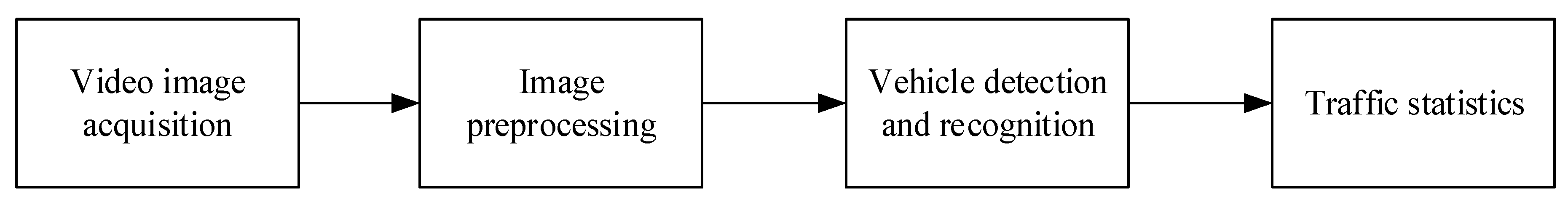
The traffic flow detection system consists of a video image acquisition module, an image pre-processing module, a vehicle detection and identification module, and a vehicle flows statistics module. The main modules of the detection system are shown in Figure 1. The core of the system is the vehicle detection and recognition module, which locates and recognizes the vehicles in the video images. In order to combine target position and recognition into one, which needs to take requirements of the speed detection and recognition accuracy into consideration, the YOLOv3 algorithm is used for the vehicles’ detection and recognition.
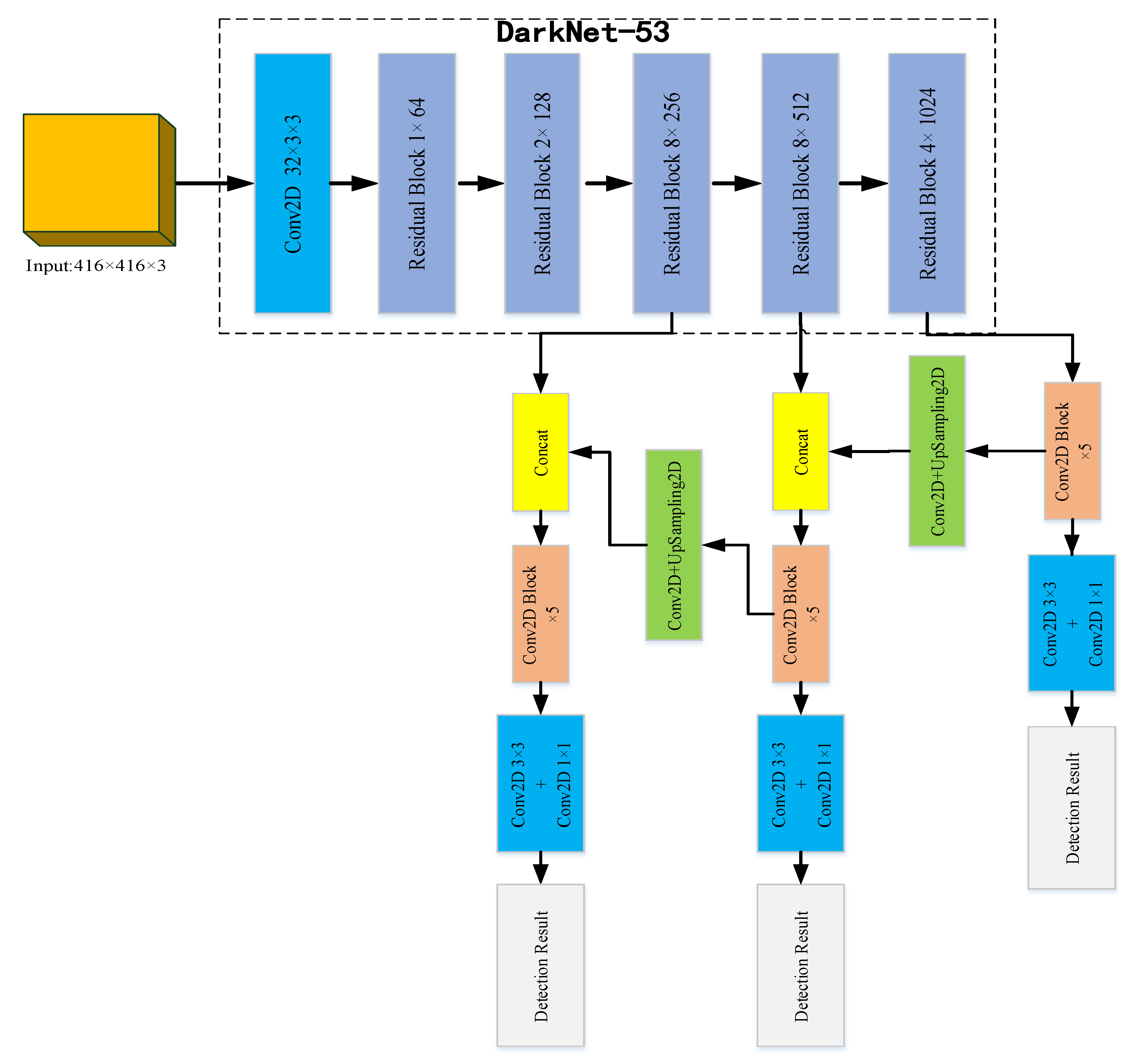
The YOLOv3 algorithm is an improvement on YOLOv1 and YOLOv2 because it has the advantages of high detection accuracy, accurate positioning, and fast speed. Especially when the multi-scale prediction methods are introduced, it can achieve the detection of small targets and has good robustness to environmental scenes, therefore, it has become a current research hotspot. The network structure of the YOLOv3 algorithm is shown in Figure 2. The residual network is mainly used to upgrade the feature extraction network, and the basic backbone network is updated from Darknet-19 to Darknet-53 to extract features and obtain deeper feature information.
The Darknet-53 network in YOLOv3 uses a large number of 1 × 1 and 3 × 3 convolutional layers in order to connect local feature interactions and its function is equivalent to the global connection of the full feature layer and the addition of shortcut connections. This operation enables us to obtain more meaningful semantic information from up-sampled features and finer-grained information from earlier feature mappings. This feature extraction network has 53 convolutional layers, which is called Darknet-53, and its structure is shown at the top in Figure 2. In Darknet-53, 1 × 1 and 3 × 3 alternating convolution kernels are used, and after each layer of convolution, the BN layer is used for normalization. The Leaky Relu function is used as the activation function, the pooling layer is discarded, and the step size of the convolution kernel is enlarged to reduce the size of the feature map. As the network structure is deeper, its ability to extract features is also enhanced. The function of the sampling layer (upsample) is to generate the small-size images by interpolation of small-size feature maps and other methods. When short connections are set up between some layers to connect low-level features with high-level ones, the fine-grained information of high-level abstract features is enhanced, and they can be used for class prediction and bounding box regression.
The YOLOv3 network prediction process is listed below:
- 1)
- First, the images of size 416 × 416 are input into the Darknet-53 network. After performing many convolutions, a feature map of size 13 × 13 is obtained, and then 7 times by 1 × 1 and 3 × 3 convolution kernels are processed to realize the first class and regression bounding box prediction.
- 2)
- The feature map with size 13 × 13 is processed 5 times by 1 × 1 and 3 × 3 convolution kernels, and then the convolution operation is performed by using 1 × 1 convolution kernel, followed by 2 times the upsampling layer, and stitching to the size on the 26 × 26 feature map. The new feature map of size 26 × 26 is then processed 7 times using 1 × 1 and 3 × 3 convolution kernels to achieve the second category and regression bounding box prediction.
- 3)
- A new feature map has a size of 26 × 26. Firstly, we use 1 × 1 and 3 × 3 convolution kernels to process 5 times, perform a double upsampling operation, and stitch it onto the feature map of size 52 × 52. Then, the feature map is processed 7 times using 1 × 1 and 3 × 3 convolution kernels to achieve the third category and regression bounding box prediction.
It can be seen from the above results, that YOLOv3 can output three feature maps of different sizes at the same time, which are 13 × 13, 26 × 26, and 52 × 52. In this way, the feature maps of different sizes are optimized for the detections of small targets, but at the same time, the detections of large targets are weakened. Each feature map predicts three regression bounding boxes at each position, each bounding box contains a target confidence value, four coordinate values, and the probability of C different edges. There are (52 × 52 + 26 × 26 + 13 × 13) × 3 = 10647 regression bounding boxes.
3. YOLO v3 Algorithm Optimization
3.1. Network Structure Optimization
During the feature extraction process of the YOLOv3 network, as the convolutional layers are deepened, the receptive field of a single neuron is gradually increasing. At the same time, the feature extraction capability is also enhanced and the extracted feature is more abstract. At this time, if the shape of the object’s feature map is blurred, the position information of the small target will be inaccurate or even lost in severe cases. Therefore, when the YOLOv3 is used for the vehicles’ detection experiment, there are a large number of vehicles in the images, the phenomenon of missed detections will occur, and the accuracies of the vehicle flow detections will be greatly reduced. To solve this problem, we introduce the idea of spatial pyramid pooling between the 5th and 6th convolutional layers of the YOLOv3 network to optimize the network structure. The SPP-net is a feature enhancement module, which extracts the main information of the feature map and performs stitching, as shown in Figure 3.
The difference between the concatenate operation and the addition operation in the module is that as the idea of the addition operation is derived from ResNet, the input feature map is added to the corresponding dimension of the output feature map, that is, y= f(x) + x. However, the idea of concatenate operation originates from the DenseNet network, and the feature graph is spliced directly according to channel dimension [19]. For example, 8 × 8 × 16 feature graph was splicing with 8×8×16 feature graph to generate 8 × 8 × 32 features.
This module draws on the idea of the spatial pyramid and realizes local and global features through the SPP module. This is why the largest pooling kernel size in the SPP module should be as close as possible or equal to the size of the feature map that needs to be pooled. After the features are fused with the global features, the expression ability of the featured maps is enriched. The main operation in the module is to down-sample the input features using pooling windows with kernel sizes of 5 × 5, 9 × 9, and 13 × 13, the pooling steps are all 1, and the pooled features are input to the concatenate operation to perform dimensional stitching. Because when the YOLOv3 network predicts the target position, the feature map of each size must be convolved 5 times by 1 × 1 and 3 × 3 convolution kernels (that is the Conv2D×5 block in Figure 2). Here, the method of directly adding the SPP module to each Conv2D × 5 structure in the figure is adopted to form an overall feature enhancement module, which can improve the network’s effect of extracting feature maps of each different size.
In summary, the network has the following characteristics after optimization:
- 1)
- The input size can be ignored and a fixed-length output can be generated to solve the problem of inconsistent input image size.
- 2)
- When the multi-level spatial multi-scale block pooling operation is used, not only a sliding window of size for the pooling operation is used, the speed of computing the entire network of features can be improved.
- 3)
- The space pyramid module divides the feature maps into different levels at different levels, calculates the features of each level, and finally fuses the features of each level together, that is, conducive to the situation of large differences in target sizes and in the images to be detected. Especially, the complex multi-target detection can be improved by YOLOv3, for that the detection accuracy has been greatly improved.
3.2. Loss Function Optimization
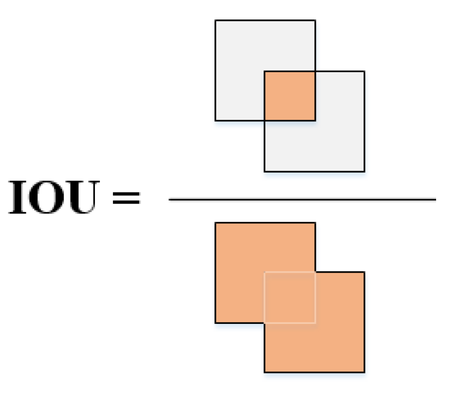
A regression bounding box is a key step in target detection and target tracking in computer vision. Traditional methods mainly improve network performance by deepening the number of layers in the backbone network and optimizing local feature extraction methods, but they often ignore the optimization of loss functions. Intersection Over Union (IOU) is a measure of overlap area, which indicates the degree of overlap between the target window generated by the model and the original labeled window [11]. It is not sensitive to the changes of scales and non-negative, and it is a common evaluation standard in target detection, also known as detection accuracy. The value of IOU is the ratio of the intersection between the detection result, the ground truth, and the union between them. The calculation diagram is shown in Figure 4.
Evaluation indicators for bounding box regression:
where Bgt = (xgt, ygt, wgt, hgt) is the real box and B= (x, y, w, h) is the prediction box. Usually, the distance between the bounding boxes is measured by the coordinates of B and Bgt using the ln-norm (n = 1 or 2) loss function. In recent years, IOU loss is usually used to improve the IOU index. The expression of IOU loss is listed as followed:
It can be seen that when the two frames do not intersect, that is, the IOU is equal to zero, which is equivalent to the loss function having no effect and cannot be learned and trained, for that, theIOU loss is only applicable to the case where the target frame overlaps. In the cases of different distances, different scales, and different aspect ratios, as IOU is used to optimize the loss function, the regression situation is often incomplete. For the case where the target boxes do not overlap, in order to optimize the IOU loss function and solve the positioning and other problems, the DIOU measurement parameters are introduced [20]. When the target box and the prediction box do not overlap, there will be a loss. The centering distance can make the prediction frame to move toward the target. The DIOU loss can directly minimize the distance between the two boxes, it means that by combining the standardized distance between the prediction box and the target box can directly minimize the normalized distance between the anchor box and the target box, for that, the loss convergence is more accurate and faster than that of the IOU.
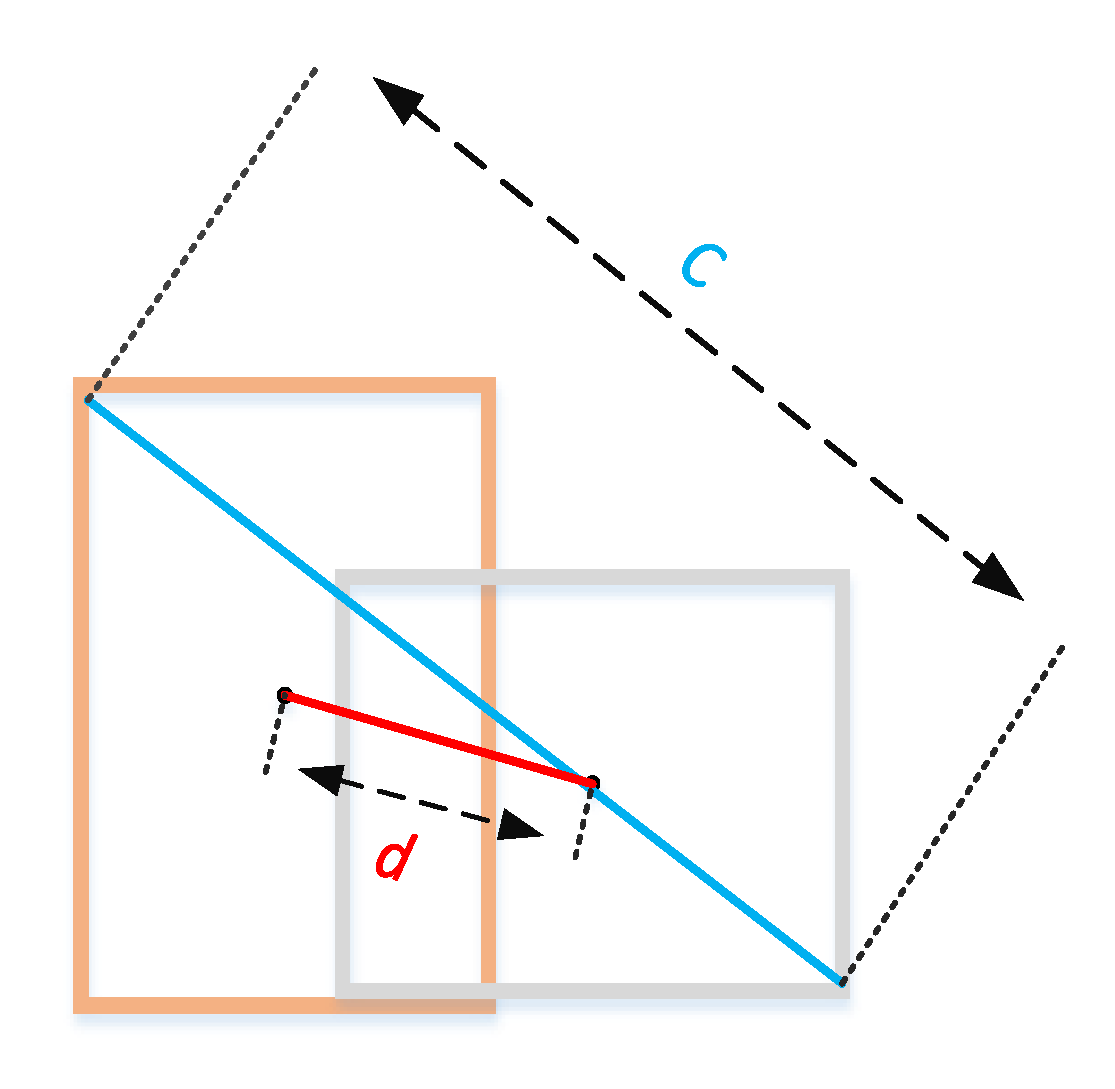
DIOU loss is mainly based on IOU loss plus a constraint term and DIOU loss is shown in Equation (3). Among this, b and bgt represent the center points of the prediction frame and the real frame, respectively, ρ represents the calculation of the Euclidean distance between the two center points. The calculation result is the value of d in Figure 5, and c represents the diagonal distance between the smallest closed area that can contain both the prediction box and the real box.
The DIOU loss can provide a moving direction for the bounding boxes when the target boxes do not overlap, which can directly minimize the distance between the two target boxes. At the same time, the regression convergence speed of DIOU loss is very fast, which solves the problem of IOU loss. In network training, DIOU loss is added to the network loss function. The value of the loss function gradually decreases with the number of iterations and the degree of overlap increases. It can effectively solve the problems of inaccurate positioning of YOLOv3. L2 regularization is used to enhance the generalization of the network to prevent the over-fitting problem, as Equation (4) shows. Where β is a hyperparameter, as the value is larger, the more important regularization will be and ∑ is the sum of squares of the ownership weight.
The network weight update is shown in Equation (5). Where µ is the learning rate of the network, regularization is actually multiplying (1–2 µβ) when the ownership weight is updated.
DIOU loss optimization can have the following effects. 1. It is similar to Generalized Intersection Over Union (GIOU) loss, but when DIOU loss does not overlap the target frame, it can still provide the moving direction for the bounding box. 2. DIOU loss can directly minimize the distance between two target boxes, so it can converge much faster than GIOU loss. 3. For the case where the two boxes are horizontal and vertical, DIOU loss can make the regression very fast, while GIOU loss is almost degraded to IOU loss [21].
In summary, for convenience of expression, the optimized algorithm model is YOLOv3-DL, where DL stands for DIOU loss. After using the above optimization, the YOLOv3-DL model can minimize the distance between two bounding boxes directly, for that, the prediction box and the target box can be completely and quickly matched together with a small number of iterations, effectively solving the positioning accuracy and speed problem existing in the YOLOv3 model. In addition, the feature enhancement methods of multi-layer extraction and fusion are adopted in the network feature extraction, which is beneficial to deal with the large difference of target size in the images to be detected. In the complex multi-target detection system such as traffic flows, this processing has greatly improved the target detection accuracy of the system. Therefore, using YOLOv3-DL in the detection system of traffic flows, at a certain speed the target vehicles can be detected with higher accuracy, and the real-time detection effects of the vehicles can be achieved, thereby, YOLOv3-DL can improve the performance of the detection system of traffic flows.
4. Making the Data Set
In order to study the monitoring of traffic flows in actual scenarios, the data source of this study uses the large-scale data set of DETection and tRACking (DETRAC) for vehicle detection and tracking. The data set is mainly derived from video images of road crossing bridges in Beijing and Tianjin, and manually labeled 8250 vehicles and 1.21 million target object frames. The shooting scenes include sunny, cloudy, rainy, and night, and the height and angle of each shot are different.
The steps for making the experimental data set of this project are as follows:
- 1)
- Collecting daytime, dusk, evening, and rainy pictures from the DETRAC data set, a total of 6203 pictures were collected;
- 2)
- Combining the 6203 pictures and the VOC_2007 data set to make a DL_CAR data set containing 26,820 pictures;
- 3)
- Randomly extracting 80% of the DL-CAR data set to make a training verification set;
- 4)
- Randomly extracting 80% from the training verification set to make the training set;
- 5)
- The remaining 20% of the DL-CAR data set is used as the verification set and test set in a 1:1 ratio;
- 6)
- Organizing your own data set according to the structure of the VOC data set. The folder structure of the VOC data set is shown in Figure 6;
- 7)
- Use OpenCV to read all the images in the folder, name them in the order of reading and unify the format to facilitate later statistics.
In this paper, the LabelImg tool is used to uniformly label each target vehicle on the pictures of the training set, validation set, and test set, and an XML file corresponding to the pictures is generated to store the labeling information for subsequent network training. After that, the XML file corresponding to the picture is generated to store the label information for subsequent network training. The actual labeling steps are:
- 1)
- Using the mouse to select and frame the target vehicle area;
- 2)
- Double-clicking to mark the corresponding target category;
- 3)
- Clicking “Save” after marking.
Each image in the training verification set initializes a 3D label in the form of [7, 7, 25] with 0, column 0 represents the confidence, column 1–4 represents the central coordinates (xc, yc, w, h), and column 5–24 represents the object class sequence number. Next, we parse the XML file and take out all target categories in the file and their coordinate values (xmin, ymin, xmax, ymax) in the upper left and lower corners, these data were then multiplied while using ratio values according to the 448 × 448 image scaling factor to obtain (x1min, y1min, x2max, y2max). Subsequently, Equation (6) is used to convert the coordinates into the form of center point coordinates, and Equation (7) is used to calculate which grid the target center falls into. In the image label, the grid confidence degree is set to 1, the coordinate of the center point is set to the calculation results of Equations (6)–(7), and the corresponding target category index is set to 1.
In order to enhance the robustness of the network, we use random horizontal flip, random cropping, random color distortion, etc. for data enhancement. We create a dictionary for each picture to store its path and label, and add all dictionaries to the list and save the list in a pkl file.
5. Experiment and Analysis of Results
5.1. Experimental Platform
The experiments in this article were performed on the Ubuntu 18.04 system (Canonical Ltd., London, United Kingdom). Under the PyCharm development environment, the program was written in Python 3.6. The YOLOv3-DL algorithm was run under the Darknet framework. The processor was an Inter Core i9-9900K CPU and the NVIDIA GeForce RTX2080Ti graphic card was used to accelerate training.
5.2. Network Training
The initialization weights for YOLOv3-DL training use the weights of the pre-trained YOLOv3 model of the VOC2007 dataset, extract the picture path and labels from the pkl file, and normalize the pixel value of the processed picture [−1,1]. We use the stochastic gradient descent method to train the algorithm 30,000 times. The learning rate is chosen to be 0.001 between 0 and 20,000 iterations. In 20000 ~ 25000 iterations, 0.1 times the current learning rate, and in 25,000 ~ 30000 iterations, the learning rate is multiplied by 0.01 times. The adjustment of the learning rate reduces training loss. Batch is set to 64 and Subdivision is set to 8. As a result, each batch will not be added to the network as a whole, but it will be divided into 8 parts. After the batch is run, it will be packaged to complete an iteration. Which can reduce the memory usage.
5.3. Analysis of Experimental Data
5.3.1. Experimental Evaluation Parameters
To verify the effectiveness of the optimization, the DL-CAR data set is used to perform the following tests, analyze the experimental data, and compare the experimental results. The problems of missed detection and false detection will happen in the monitoring processes of traffic flows. In this experiment, Precision, Recall, and mAP are used as evaluation parameters. The “Precision” (accuracy) is the ratio of the number of correctly detected statistical vehicles to the total number of detected statistical vehicles. The “Recall” (recall rate) is the ratio of the number of correctly detected statistical vehicles to the total number of vehicles in the data set. The calculation method is shown in Equations (8)–(10).
In these formulas, True Positive (TP) indicates the number of correctly detected vehicles, True Negative (TN) indicates the number of correctly detected backgrounds, False Positive (FP) indicates the number of incorrect detections, and False Negative (FN) indicates the number of missed detections, respectively. In Equation (10), xr is the maximum value of the recall rate greater than the corresponding precision rate of the interval segment, and then the average value of the maximum value of 11 points is calculated. In practice, we do not directly calculate the PR curve but smooth the PR curve. That is, for each point on the PR curve, the value of Precision is the value of the largest Precision to the right of that point.
5.3.2. Comparative analysis of Different Algorithm Experiments
The XML file is parsed in the image folder of the dataset and the actual number of vehicles is counted in the dataset. The optimized YOLOv3-DL model is used to detect the number of vehicles in the statistical data set, which is called the number of statistics. The Precision, Recall, and Accuracy of vehicle statistics was calculated and compared with the YOLOv3 model. The experimental results are shown in Table 1 and Table 2.
From the results in Table 1 and Table 2, under the presupposition, we found that the actual vehicle base of the data set is large. Compared with the results of the YOLOv3 model, the statistical accuracy of the YOLOv3-DL model is increased by 3.86% and the recall rate is increased by 3.65%. In the data set labeling, we do not fully label the vehicles that are far away, the targets are small, and the images are blurred. The actual number in the table represents the total number of vehicles labeled with the Labellmg tool when our previous data set is prepared. In Table 1 and Table 2, the number of statistical vehicles in the model data set is higher than the actual number of vehicles. It can be explained that the above two models can be used to detect vehicles with large targets and vehicles with small targets, so the above table appears. The number of statistics in China is higher than the actual number, which indirectly shows that the above model has better generalization in vehicles’ detection.
5.3.3. Comparative Analysis of Experiments in Different Scenarios
In order to study the adaptability of the optimization model to multi-scenario and multi-weather traffic detections, 1000 sets of pictures were taken for each scene through the self-made datasets of sunny, cloudy, rainy, and night, then they were tested with YOLOv3 and YOLOv3-DL models. The experimental results are shown in Table 3 and Table 4.
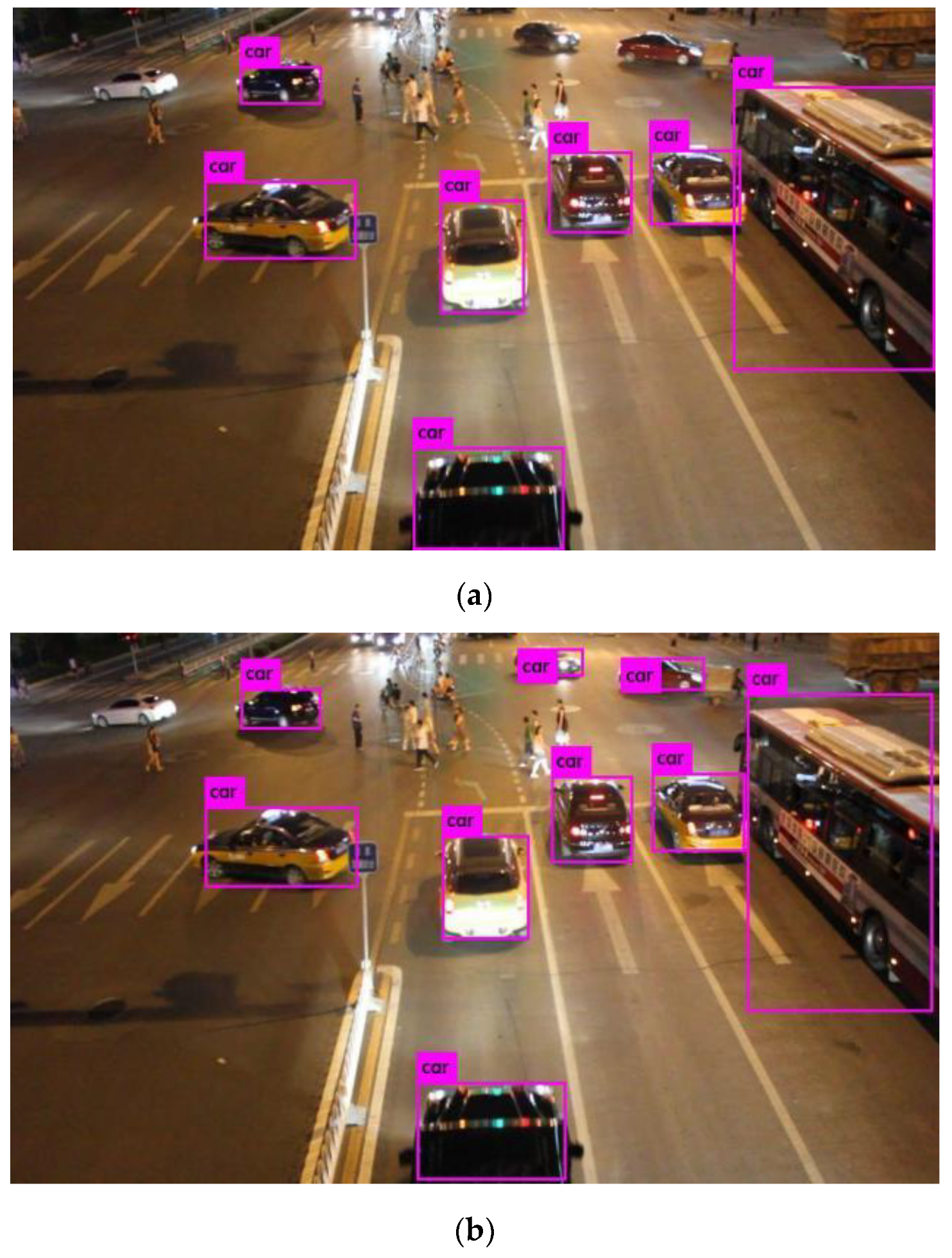
Using the DIOU-optimized network model YOLOv3-DL, we find that the statistical average accuracy is improved to 4.53% and the network performance has improved significantly. For different scenes and weathers, its adaptability has been improved as compared to that of YOLOv3, which can more accurately detect vehicles and be used for monitoring tasks of traffic flows. Based on the results of experimental tests on multiple scenes and weathers, some vehicles will be missed in the detections of YOLOv3 before optimization, which leads to a decline in statistical accuracy, as shown in Figure 7.
5.3.4. Video Stream Experimental Data Analysis
In order to test the detection capability of the YOLOv3-DL algorithm in the video stream, we collected vehicles’ driving videos for experiments in a variety of different scenarios and different weathers. The length of each collected video is uniformly 40 s. For further comparison, we take a Test-1 video at the roadside on a clear day at dusk, a Test-2 video on the flyover at noon on a clear day, and a Test-3 video on the sidewalk on a cloudy morning. The test results shown in Table 5 and Table 6 have also presented that even in different weather conditions, the accuracy rates of the YOLOv3-DL algorithm are higher than those of the YOLOv3 algorithm.
The test results show that it takes an average of 25 ms to count the vehicles per frame image, and the monitoring of traffic flows using the YOLOv3-DL algorithm is almost equal to the real traffic flow. As compared with the previous results of YOLOv3, the video monitoring accuracy rate of traffic flows has been improved, and we also note that the video collection location should not be too high and the field of view should not be too large. Because when the location is too high, it may cause missed detection, and the field of vision will cause false detection. The average accuracy rates of traffic statistics in Table 5 and Table 6 are 90.8% and 98.8%, respectively, and the average statistical times of YOLOv3 and YOLOv3-DL are 32 ms and 25 ms, respectively. When these results are compared with other monitoring algorithms of traffic flows, such as Faster R-CNN and SSD, as the results in Table 7 show, the YOLOv3-DL algorithm has the maximum accuracy rate and shortest monitoring time.
6. Conclusions
Due to the limitations of the YOLOv3 model, when more vehicles are close to each other in the images or the vehicles’ target size is not the same, it will have missed detections and positioning problems, further affecting the accuracy rates of traffic flow statistics and prediction information. By using the YOLOv3-Dl algorithm and optimized by DIOU, the traffic flow statistics with a high accuracy rate can be generated, and the results obtained after adjusting the threshold parameters are very close to the actual number of vehicles. After optimization, the algorithm can reliably conduct the monitoring of traffic flows and statistical analysis in a variety of scenarios and weather conditions. The experimental results show that the YOLOv3 model needs to be further improved in real-time and accuracy rate of traffic monitoring. Therefore, we will introduce the pyramid space module (i) the feature extraction of the network structure to optimize YOLOv3 themselves, (ii) DIOU loss to solve the problem of unbalanced category, (iii) during the training of batch standardization to further improve its adaptability to all kinds of weathers and scenarios. In this experiment, we can see on the test set, the detection accuracy rate of the YOLOv3-DL algorithm increased by 3.86% as compared with that of YOLOv3, and under different environmental conditions, the detection accuracy rate of the YOLOv3-DL algorithm increased by 4.53% as compared with that of YOLOv3. In the video monitoring of traffic flows, as compared with the previous Faster R-CNN, SSD, and YOLOv3 algorithms, the YOLOv3-DL algorithm achieves the accuracy rate of 98.8% and the detection speed of 25 ms at the same time, which meets the requirements of high precision and fast speed required by monitoring of traffic flows and further improves the real-time detection system of traffic flows.
Author Contributions
Investigation, Y.-Q.H., J.-C.Z. and C.-F.Y.; Methodology, Y.-Q.H., J.-C.Z., S.-D.S., and J.L.; Formal analysis, Y.-Q.H., S.-D.S., C.-F.Y., and J.L.; Writing—original draft preparation, Y.-Q.H., J.-C.Z., S.-D.S., C.-F.Y., and J.L.; Writing-review and editing, C.-F.Y., Y.-Q.H. and J.-C.Z. All authors have read and agreed to the published version of the manuscript.
Acknowledgments
This work was supported by key project of Fujian science and technology plan (No. 2017h0028); Fund project of Jimei University (No. zp2020042). This work was also supported by projects under No. MOST 108-2221-E-390-005 and MOST 108-2622-E-390-002-CC3.
Conflicts of Interest
The authors declare no conflict of interest.
References
- Liu, Y. Big Data Technology and Its Analysis of Application in Urban Intelligent Transportation System. In Proceedings of the International Conference on Intelligent Transportation, Big Data & Smart City (ICITBS), Xiamen, China, 25–26 January 2018; pp. 17–19. [Google Scholar]
- Xu, Y.Z.; Yu, G.Z.; Wang, Y.P.; Wu, X.K.; Ma, Y.L. A Hybrid Vehicle Detection Method Based on Viola-Jones and HOG + SVM from UAV Images. Sensors 2016, 16, 1325–1348. [Google Scholar] [CrossRef] [PubMed] [Green Version]
- Qiu, Q.J.; Yong, L.; Cai, D.W. Vehicle detection based on LBP features of the Haar-like Characteristics. In Proceedings of the 11th World Congress on Intelligent Control and Automation, Shenyang, China, 29 June–4 July 2014; pp. 1050–1055. [Google Scholar]
- Felzenszwalb, P.F.; Girshick, R.B.; Mcallester, D.; Ramanan, D. Object Detection with Discriminatively Trained Part-Based Models. IEEE Trans. Softw. Eng. 2010, 32, 1627–1645. [Google Scholar] [CrossRef] [PubMed] [Green Version]
- Prakash, J.S.; Vignesh, K.A.; Ashok, C.; Adithyan, R. Multi class Support Vector Machines classifier for machine vision application. In Proceedings of the International Conference on Machine Vision and Image Processing (MVIP), Taipei, Taiwan, 14–15 December 2012; pp. 197–199. [Google Scholar]
- Kenan, M.U.; Hui, F.; Zhao, X.; Prehofer, C. Multiscale edge fusion for vehicle detection based on difference of Gaussian. Opt.-Int. J. Light Electron Opt. 2016, 127, 4794–4798. [Google Scholar]
- Lecun, Y.; Bottou, L.; Bengio, Y.; Haffner, P. Gradient-based learning applied to document recognition. Proc. IEEE 1998, 86, 2278–2324. [Google Scholar] [CrossRef] [Green Version]
- Girshick, R.; Donahue, J.; Darrell, T.; Malik, J. Rich Feature Hierarchies for Accurate Object Detection and Semantic Segmentation. In Proceedings of the IEEE Conference on Computer Vision and Pattern Recognition, Columbus, OH, USA, 24–27 June 2014; pp. 580–587. [Google Scholar]
- He, K.; Zhang, X.; Ren, S.; Sun, J. Spatial Pyramid Pooling in Deep Convolutional Networks for Visual Recognition. IEEE Trans. Pattern Anal. Mach. Intell. 2015, 37, 1904–1916. [Google Scholar] [CrossRef] [PubMed] [Green Version]
- Thakar, V.; Saini, H.; Ahmed, W.; Soltani, M.M.; Aly, A.; Yu, J.Y. Efficient Single-Shot Multibox Detector for Construction Site Monitoring. In Proceedings of the 4th IEEE International Smart Cities Conference (ISC2), Kansas City, MO, USA, 16–19 September 2018; pp. 1–6. [Google Scholar]
- Redmon, J.; Divvala, S.; Girshick, R.; Farhadi, A. You Only Look Once: Unified, Real-Time Object Detection. In Proceedings of the IEEE Conference on Computer Vision and Pattern Recognition (CVPR), Las Vegas, NV, USA, 27–30 June 2016; pp. 779–788. [Google Scholar]
- Redmon, J.; Farhadi, A. YOLO9000: Better, Faster, Stronger. In Proceedings of the IEEE Conference on Computer Vision and Pattern Recognition (CVPR), Honolulu, HI, USA, 21–26 July 2017; pp. 6517–6525. [Google Scholar]
- Redmon, J.; Farhadi, A. YOLOv3: An Incremental Improvement. In Proceedings of the IEEE Conference on Computer Vision and Pattern Recognition (CVPR), Salt Lake City, UT, USA, 18–22 June 2018; pp. 1854–1862. [Google Scholar]
- Liu, J.; Huang, Y.; Peng, J.; Yao, J.; Wang, L. Fast Object Detection at Constrained Energy. IEEE Trans. Emerg. Top. Comput. 2018, 6, 409–416. [Google Scholar] [CrossRef]
- Ren, S.; He, K.; Girshick, R.; Sun, J. Faster R-CNN: Towards Real-Time Object Detection with Region Proposal Networks. IEEE Trans. Pattern Anal. Mach. Intell. 2017, 39, 1137–1149. [Google Scholar] [CrossRef] [PubMed] [Green Version]
- Tesema, F.B.; Lin, J.; Ou, J.; Wu, H.; Zhu, W. Feature Fusing of Feature Pyramid Network for Multi-Scale Pedestrian Detection. In Proceedings of the 15th International Computer Conference on Wavelet Active Media Technology and Information Processing (ICCWAMTIP), Chengdu, China, 14–16 December 2018; pp. 10–13. [Google Scholar]
- He, K.; Zhang, X.; Ren, S.; Sun, J. Deep Residual Learning for Image Recognition. In Proceedings of the IEEE Conference on Computer Vision and Pattern Recognition (CVPR), Las Vegas, NV, USA, 10–13 December 2016; pp. 770–778. [Google Scholar]
- Cao, C.Y.; Zheng, J.C.; Huang, Y.Q.; Liu, J.; Yang, C.F. Investigation of a Promoted You Only Look Once Algorithm and Its Application in Traffic Flow Monitoring. Appl. Sci. 2019, 9, 3619. [Google Scholar] [CrossRef] [Green Version]
- Huang, G.; Liu, Z.; Maaten, L.V.D.; Weinberger, K.Q. Densely Connected Convolutional Networks. In Proceedings of the IEEE Conference on Computer Vision and Pattern Recognition, Honolulu, HI, USA, 21–26 July 2017; pp. 234–258. [Google Scholar]
- Zheng, Z.; Wang, P.; Liu, W.; Li, J.; Ye, R.; Ren, D. Distance-IoU Loss: Faster and Better Learning for Bounding Box Regression. 2019, pp. 1458–1467. Available online: https://arxiv.org/abs/1911.08287 (accessed on 9 March 2020).
- Rezatofighi, H.; Tsoi, N.; Gwak, J.; Sadeghian, A.; Reid, I.; Savarese, S. Generalized Intersection Over Union: A Metric and a Loss for Bounding Box Regression. In Proceedings of the 32nd IEEE/CVF Conference on Computer Vision and Pattern Recognition (CVPR), Long Beach, CA, USA, 16–21 June 2019; pp. 658–666. [Google Scholar]
Figure 1.
Detection System Process.

Figure 2.
YOLOv3 network structure diagram.

Figure 3.
Spatial Pyramid Pooling Module.

Figure 4.
Intersection Over Union (IOU) Calculation.

Figure 5.
Boundary Box Regression Diagram.

Figure 6.
VOC Data Set Structure.

Figure 7.
Comparison of Vehicle Detection Based on Optimized Models (a) YOLOv3 algorithm detection results and (b) YOLOv3-DL algorithm detection results.
Figure 7.
Comparison of Vehicle Detection Based on Optimized Models (a) YOLOv3 algorithm detection results and (b) YOLOv3-DL algorithm detection results.


Table 1.
YOLOv3 general model traffic statistics.
| Data Sets | Number of Actual | Number of Statistics | Precision (%) | Recall (%) | Accuracy Rate (%) |
|---|---|---|---|---|---|
| Training set | 11,1351 | 11,2422 | 94.23 | 95.14 | 95.14 |
| Training verification set | 139098 | 14,0427 | 94.24 | 95.14 | 95.14 |
| Verification set | 27,747 | 27,982 | 94.36 | 95.16 | 95.16 |
| Test set | 34,760 | 35,416 | 93.22 | 94.98 | 95.01 |
Table 2.
YOLOv3-DL general model traffic statistics.
| Data Sets | Number of Actual | Number of Statistics | Precision (%) | Recall (%) | Accuracy Rate (%) |
|---|---|---|---|---|---|
| Training set | 11,1351 | 11,3929 | 96.73 | 98.97 | 98.97 |
| Training verification set | 13,9098 | 14,0937 | 96.77 | 98.05 | 98.97 |
| Verification set | 27,747 | 28,374 | 96.92 | 99.11 | 99.11 |
| Test set | 34,760 | 3,5870 | 95.82 | 98.88 | 98.83 |
Table 3.
YOLOv3 multi-environment traffic statistics.
| Data Sets | Number of Actual | Number of Statistics | Precision (%) | Recall (%) | Accuracy Rate (%) |
|---|---|---|---|---|---|
| Sunny | 6823 | 6837 | 94.85 | 95.05 | 95.05 |
| Cloudy | 5922 | 5968 | 94.52 | 95.26 | 95.25 |
| Rainy | 8517 | 8629 | 93.49 | 94.73 | 94.69 |
| Night | 5731 | 5825 | 93.74 | 95.27 | 95.26 |
Table 4.
YOLOv3-DL multi-environment traffic statistics.
| Data Sets | Number of Actual | Number of Statistics | Precision (%) | Recall (%) | Accuracy Rate (%) |
|---|---|---|---|---|---|
| Sunny | 6823 | 6861 | 98.33 | 98.87 | 98.91 |
| Cloudy | 5922 | 6031 | 98.17 | 99.99 | 99.97 |
| Rainy | 8517 | 8694 | 97.59 | 99.61 | 99.56 |
| Night | 5731 | 5852 | 97.88 | 99.95 | 99.94 |
Table 5.
YOLOv3 video traffic monitoring.
| Video | Number of Actual | Number of Statistics | Accuracy (%) |
|---|---|---|---|
| Test-1.mp4 | 50 | 44 | 88 |
| Test-2.mp4 | 67 | 62 | 92.5 |
| Test-3.mp4 | 25 | 23 | 92 |
Table 6.
YOLOv3-DL video traffic monitoring.
| Video | Number of Actual | Number of Statistics | Accuracy (%) |
|---|---|---|---|
| Test-1.mp4 | 50 | 49 | 98 |
| Test-2.mp4 | 67 | 66 | 98.5 |
| Test-3.mp4 | 25 | 25 | 100 |
Table 7.
Different algorithm traffic monitoring.
| Algorithm | Accuracy (%) | Time/ms |
|---|---|---|
| ViBe | 96.2 | 158 |
| Faster R-CNN | 83.5 | 85 |
| SSD | 85.8 | 54 |
| YOLOv3 | 90.8 | 32 |
| YOLOv3-DL | 98.8 | 25 |
© 2020 by the authors. Licensee MDPI, Basel, Switzerland. This article is an open access article distributed under the terms and conditions of the Creative Commons Attribution (CC BY) license (http://creativecommons.org/licenses/by/4.0/).
Share and Cite
MDPI and ACS Style
Huang, Y.-Q.; Zheng, J.-C.; Sun, S.-D.; Yang, C.-F.; Liu, J. Optimized YOLOv3 Algorithm and Its Application in Traffic Flow Detections. Appl. Sci. 2020, 10, 3079. https://doi.org/10.3390/app10093079
AMA Style
Huang Y-Q, Zheng J-C, Sun S-D, Yang C-F, Liu J. Optimized YOLOv3 Algorithm and Its Application in Traffic Flow Detections. Applied Sciences. 2020; 10(9):3079. https://doi.org/10.3390/app10093079
Chicago/Turabian StyleHuang, Yi-Qi, Jia-Chun Zheng, Shi-Dan Sun, Cheng-Fu Yang, and Jing Liu. 2020. "Optimized YOLOv3 Algorithm and Its Application in Traffic Flow Detections" Applied Sciences 10, no. 9: 3079. https://doi.org/10.3390/app10093079
Note that from the first issue of 2016, this journal uses article numbers instead of page numbers. See further details here.