Investigation on Sensorless Estimating Method and Characteristics of Friction for Ball Screw System


1
School of Mechanical Engineering and Automation, Liaoning University of Technology, Jinzhou 121001, China
2
Weichai Power Co., Ltd., Weifang 261061, China
3
School of Mechanical Engineering and Automation, Northeastern University, Shenyang 110819, China
*
Author to whom correspondence should be addressed.
Appl. Sci. 2020, 10(9), 3122; https://doi.org/10.3390/app10093122
Submission received: 14 April 2020
/
Revised: 25 April 2020
/
Accepted: 27 April 2020
/
Published: 29 April 2020
Abstract
:In this study, a novel sensorless method is developed to estimate the friction in a ball screw system using asynchronous experimental data for a worktable position (WP) and the servo motor torque current (SMTC), which is collected by the FOCAS library functions from a FANUC digital control system. The corresponding time stamps are retrieved by a high-resolution performance counter in Windows. The fluctuations in friction over the whole travel distance of the worktable (WTDOW) are analyzed using a piecewise polynomial fitting algorithm to extract the instantaneous average friction value (IAFV) and the friction fluctuating signal (FFS). The IAFVs can describe the effect of the WP and the pitch errors of the shaft on the friction. The FFT results of the FFS show that the friction depends on the rolling tool, the pitch of the shaft and the refeeding of the balls in the ball screw and linear ball rail guides. The experimental results show that the estimated friction can capture the characteristic spectra of the FFS. The effects of the feed velocity and direction, the effects of the WP on the IAFV, and the frequencies and amplitudes of the significant FFT components are discussed. The nonuniform pitch errors of the shaft impact the repeatability of the IAFVs at a given WP. The variations in the mean value of the IAFVs with the feed velocity for tests at a fixed WP show nonconventional Stribeck behavior. These results also demonstrate that the friction force varies with the WP, which is not captured by Stribeck characteristics. This study provides an effective method to evaluate the performance of a ball screw system and to predict the friction in that system without the use of sensors.
1. Introduction
In high-precision positioning applications, the friction in the feed drive system can cause significant positioning error [1,2]. The successful compensation of friction is essential for accurate motion control. However, friction is caused by extremely complex interactions between the surface and near-surface regions of two interacting materials, such as in lubrication, and the surface textures of the bodies in contact with each other [3]. These factors make the friction of feed drive systems undesirably nonlinear and difficult to model. Therefore, a comprehensive understanding of the friction behavior of a feed drive system is required to develop a good friction model for accurate motion control and compensation design.
There are two important friction behaviors in a ball screw system: (1) elastic deformation and an increase in the friction of the pre-sliding regime and (2) plastic deformation and an increase in static friction [4].
In the pre-sliding regime, frictional forces dominate the hysteretic nonlocal memory of the displacement [5]. These forces act together with the stick-slip in the contact between the drive and the balls to generate an asymmetric path for the driving force [6]. In addition, basic parameters, such as the contact angle, the ball diameter, and the preload, are nonlinearly related to the ball screw friction [7]. The LuGre model describes experimentally observed friction behaviors, which include the Stribeck effect, spring-like characteristics for stiction and a varying breakaway forces [8]. Tjahjowidodo et al. [9] adopted various friction models, ranging from the Coulomb model to the generalized Maxwell-slip (GMS) model, to describe friction compensation. The Coulomb model and the Stribeck effect were found to be effective for describing motion with a high displacement, whereas the GMS model was effective for describing friction behavior in the pre-sliding regime. The complexity of the structures of these different friction models increases from the Coulomb model to the GMS model. A single experiment can be used to identify a model for friction behavior. However, the selection of the excitation signal is a critical component of this identification process for a single experiment [9]. Yeh and Su observed periodic friction for which the fast Fourier transform (FFT) results included the 1-, 2-, 3- and 4-component amplitudes of the position frequency [10]. Yamada and Kakinuma observed that the instantaneous average friction values (IAFVs) varied with the worktable position (WP) [11]. Manufacturing tolerances and incorrect alignment of the linear guides and the ball screw can cause preloading over the useful travel of the screw to differ from the specified value [12]. As a result, the friction varies over the useful travel of a ball screw. Therefore, the friction characteristics of a ball screw drive system are not only foundational for developing a friction model for compensation control but can also be used as a technical specification for evaluating the manufacturing tolerances and assembly accuracy of the components in a system. However, there have been no studies on how the friction of a ball screw feed drive system depends on position. An experimental system with a measurement apparatus needs to be developed to specifically address this issue. It is difficult to apply the results of the aforementioned studies to evaluate the quality of parts and their assembly and to predict the compensation friction for the ball screw drive systems that are used in commercial machine tools.
In this study, a sensorless method is developed for friction estimation, and the friction characteristics of a ball screw drive system in a commercial machine tool are analyzed. This paper is organized as follows: In Section 2, the experimental apparatus and procedure are described. In Section 3, an equation for describing the ball screw system is presented, and the corresponding friction is estimated. In Section 4, the position- and velocity-dependent characteristics of the IAFV and the spectra of the FFS are discussed, respectively. Finally, the conclusions are presented in Section 5.
2. Experimental Setup and Data Collection
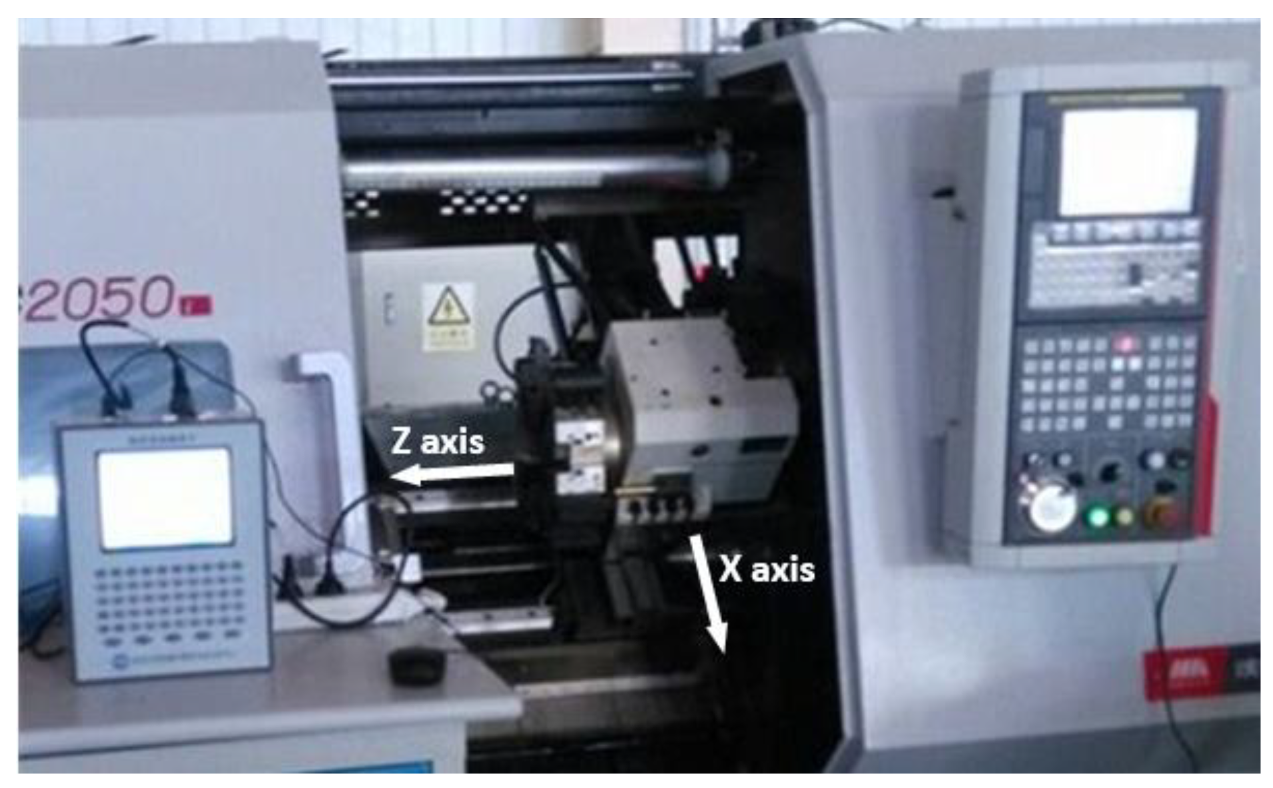
This experimental study was conducted using a lathe with a Fanuc 0i Mate-TD, as illustrated in Figure 1, which consists of two worktables that are referenced to the x-axis and the z-axis. The z-axis worktable was installed on a 45°-slant bed by a pair of linear ball guides. The x-axis worktable was installed on the z-axis worktable using another pair of linear ball guides.
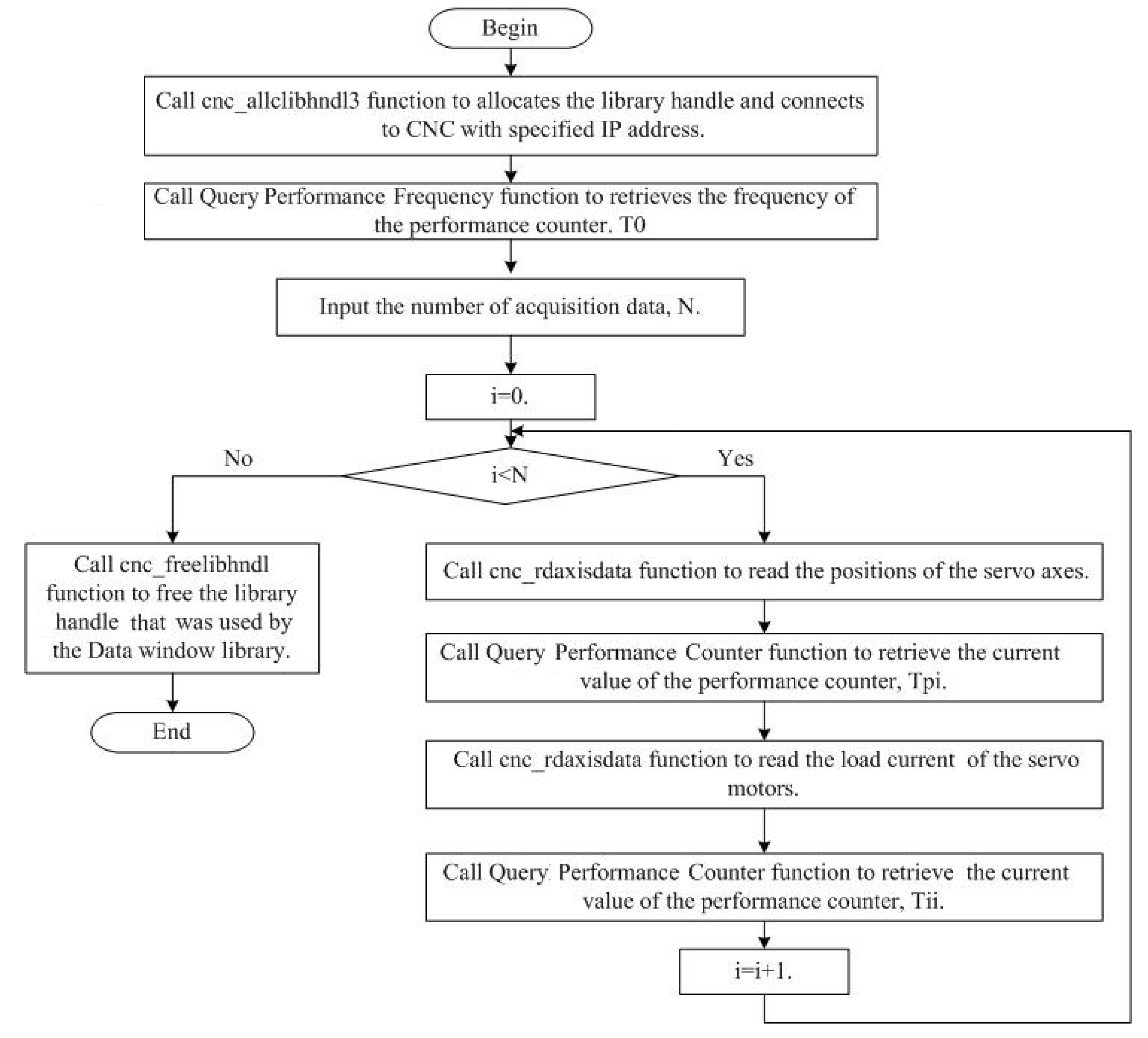
The servo data read is facilitated by the remote functions of the CNC Fanuc 0i Mate-TD via the FOCAS1/Ethernet protocol. This API and the FOCAS1/Ethernet driver installed in the CNC, which is accessed through a TCP/IP socket (192.168.1.1, 8193) using an Ethernet communication network, enables an application on a personal computer to execute the function, cnc_rdaxisdata, to read various data related to the servo axis or the spindle axis. Figure 2 shows the current communication ability of the CNC Fanuc 0i Mate-TD, which contains the Ethernet card and the FOCAS1 communication protocol [13]. Here, a PC104 bus computer is used to execute an application program on a Microsoft Windows XP system to read the positions of the servo axes and the servo motor torque current (SMTC). The program was written in the C language. The data for the servo axes that are retrieved from the CNC Fanuc 0i Mate-TD do not have time stamps. Thus, the motion parameters of the worktable cannot be calculated. However, Microsoft Windows XP provides APIs that can be used to acquire high-resolution time stamps or measure time intervals. The program uses the functions Query Performance Frequency() and Query Performance Counter() to mark the time stamps after the retrieval of a piece of data related to the servo axes. These operations for performance measurement include the computation of the response time of the CNC system and latency, as well as the execution of the profiling code, and the time interval between the ends of the events for executing the function, cnc_rdaxisdata, twice and can be independent of any external time of day [14]. Hence, these intervals can be defined as the intervals between two data points that are related to the servo axes. Figure 3 provides a block diagram of the application program.
In Figure 3, the interval of one loop is approximately 70 to 73 ms. Prior to conducting the experiment, the runtime of the NC program was evaluated to determine the number of acquisition data, thereby ensuring that the runtime of the NC program would be less that of the acquisition data application program on the PC104 computer. Here, only the z-axis worktable is investigated, and its specifications are listed in Table 1. The experimental procedure is given below.
- (1)
- Manually adjust the z-axis worktable using the control panel to locate the starting position for the experiment.
- (2)
- Run the application program on the PC104 computer and ensure that the PC104 computer connects successfully to the CNC Fanuc 0i Mate-TD.
- (3)
- Input the number of acquisition data, N, and begin data sampling.
- (4)
- Run the NC program on the CNC Fanuc 0i Mate-TD to perform an idling test.
The application program on the PC104 computer ends after the lathe stops. Then, the time stamps relating the WP and the SMTC are redefined. In the acquisition data, the values of the WP change from a series of start positions to intermediate positions to a series of end positions. The time stamp that relates the last value of the start position for the worktable is referred to as the time start point, and the time stamp that relates the first value of the end position for the worktable is considered to be the end of the experiment. The time that relates the WP to the SMTC is the difference between their corresponding time stamps and the start point.
3. Sensorless Friction Estimation
3.1. Equation of Motion for the Feed Drive System
Here, we use the feed drive system of the z-axis worktable as an example to estimate the friction force. As shown in Figure 4, this feed drive system consists of an a.c. servo motor, a coupler, a pair of linear ball guides, a ball screw and nut, bearings, a lathe bed saddle, and a turret. The ball screw on the z-axis is supported by a pair of angular contact ball bearings at each end. The inertia of the motor armature, the coupler, and the ball screw are lumped together into an equivalent inertial term, J. The viscous damping of the bearings is lumped into an equivalent term, B. Neglecting the deformations of the lead screw bar and the screw-nut contact, the equation of motion for the motor shaft can be expressed as follows:
where is the motor constant of the servo motor; is the SMTC; , and are the angular displacement, the angular velocity and the angular acceleration of the motor shaft, respectively; and is the torque with which the screw-nut drives the z-axis worktable.
Let p denote the lead of the screw; then, the relationship between the angular displacement, , and the displacement of the worktable, z, can be expressed as follows:
and the force, , with which the screw nut drives the worktable can be expressed as
Then, the equation for the worktable is expressed as
where denotes the mass of the worktable; denotes the friction force of the worktable; and denotes the acceleration of the worktable along the z-direction.
Substituting Equations (2)–(4) into Equation (1) and rearranging them yields the following equation of motion for the feed drive system:
3.2. Algorithm of Sensorless Friction Estimation
In the operation of a feed drive servomechanism, the friction and the screw pretension vary instantaneously [10,11,12]. As a result, the velocity of the worktable also varies instantaneously [15,16]. If the velocity and acceleration of the worktable are experimentally measured, the friction can be determined by solving Equation (5). However, only data for the WP versus time are obtained in Section 2. The experimental data are sampled as given below.
The data knots for the WP are
The data knots for the SMTC are
In the experimental data, , , and range from 70 to 75 ms. The experimental data are interpolated as time-continuous functions of the WP and the SMTC using a cubic spline algorithm. The velocity and acceleration of the worktable are then determined by finding the first and second derivatives of the time-continuous function of the WP, respectively. For a feed servomechanism, the friction force and the screw pretension vary periodically with the WP, and their respective spectra include multiple frequency components of the positioning frequency [10,11]. To overcome the effect of the worktable velocity on the estimation of the friction force, the velocity, and acceleration for the worktable, the SMTC are resampled with one mth of the screw lead as the sampling period. The experimental data are processed using MATLAB, as described below.
- (1)
- Cubic spline functions are used to interpolate between all of pairs of knots, and , and between and , to yield time-continuous functions for the WP and the SMTC, and , respectively.
- (2)
- The first and second derivatives of the time spline function of the WP are calculated to yield the velocity and acceleration functions of the worktable, and , respectively.
- (3)
- All of the knots, and , are interpolated to yield the position-dependent run time of the worktable, .
- (4)
- The WP is sampled with one mth of the screw lead as the sampling period to yield two arrays of position sampling points, for the forward experiment and for the backward experiment.
- (5)
- The resampling time points, , are determined by using the function and the position sampling point, Z.
- (6)
- The velocity and acceleration for the worktable and the SMTC that correspond to the resampling time points are determined by using the functions , and .
- (7)
- The friction force is calculated from Equation (5).
The starting position of the worktable is manually adjusted to the absolute zero of the lathe. The end point is fixed at 410 mm of the absolute position of the worktable, and the feed speed is 5 mm/min. To estimate the friction of the servomechanism, a NC program automatically controls the worktable to move from the start point to the end point with a residence time of one second, after which the worktable returns to the start point. The sampling cycle of the screw length is set at p/1024 to resample the velocity and acceleration of the worktable and the SMTC. In Figure 5, the variation in the estimated friction with the WP is shown for both the forward and backward motion of the worktable. The estimated friction fluctuates significantly around the IAFVs with the WP, and the IAFVs also vary with the WP.
4. Friction Characteristics Analysis
4.1. Position-Dependent Friction Characteristics
4.1.1. Instantaneous Average Friction
As mentioned above, the estimated friction oscillates around the IAFV, which also varies with the WP. Here, the IAFVs are assumed to be polynomial functions of the WP:
The coefficients of Equation (6) are determined by using the least squares polynomial fitting algorithm. Table 2 lists the average standard deviations for different orders of polynomials over the whole travel distance of the worktable (WTDOW). The quartic polynomial () exhibits the lowest average standard deviation for both the forward and backward feeds of all the polynomial orders and is therefore used to fit the IAFV.
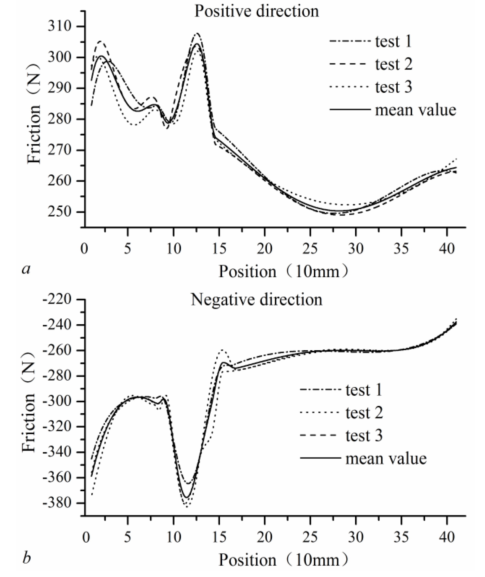
In Figure 6a,b, the estimated friction and its IAFV are compared by using dotted lines to show the polynomial fits over the WTDOW for the forward and backward feeds. The estimated friction exhibits different fluctuation patterns over the WTDOW; thus, a single quartic polynomial (as shown by the dotted lines) cannot fit the IAFVs well. To match the fluctuation patterns of the estimated friction, the WTDOW is divided into three intervals: Interval 1, which ranges from 0 to 85 mm; Interval 2, which ranges from 85 to 150 mm; and Interval 3, which ranges from 150 to 410 mm. The friction signals fluctuate smoothly over Intervals 1 and 3. Hence, the quartic polynomial () is used to fit the IAFVs for these intervals. The estimated friction exhibits anomalous fluctuations over Interval 2: Here, a quintic polynomial (m = 5) is used to describe the IAFVs. A global continuous curve fitting method in which the piecewise least squares method is combined with global continuity [17] is used for the continuous and smooth sections of the IAFV curve. The results are plotted as solid lines in Figure 6. The piecewise polynomials clearly describe the fluctuation characteristics of the IAFVs better than a single polynomial fit over the entire WTDOW.
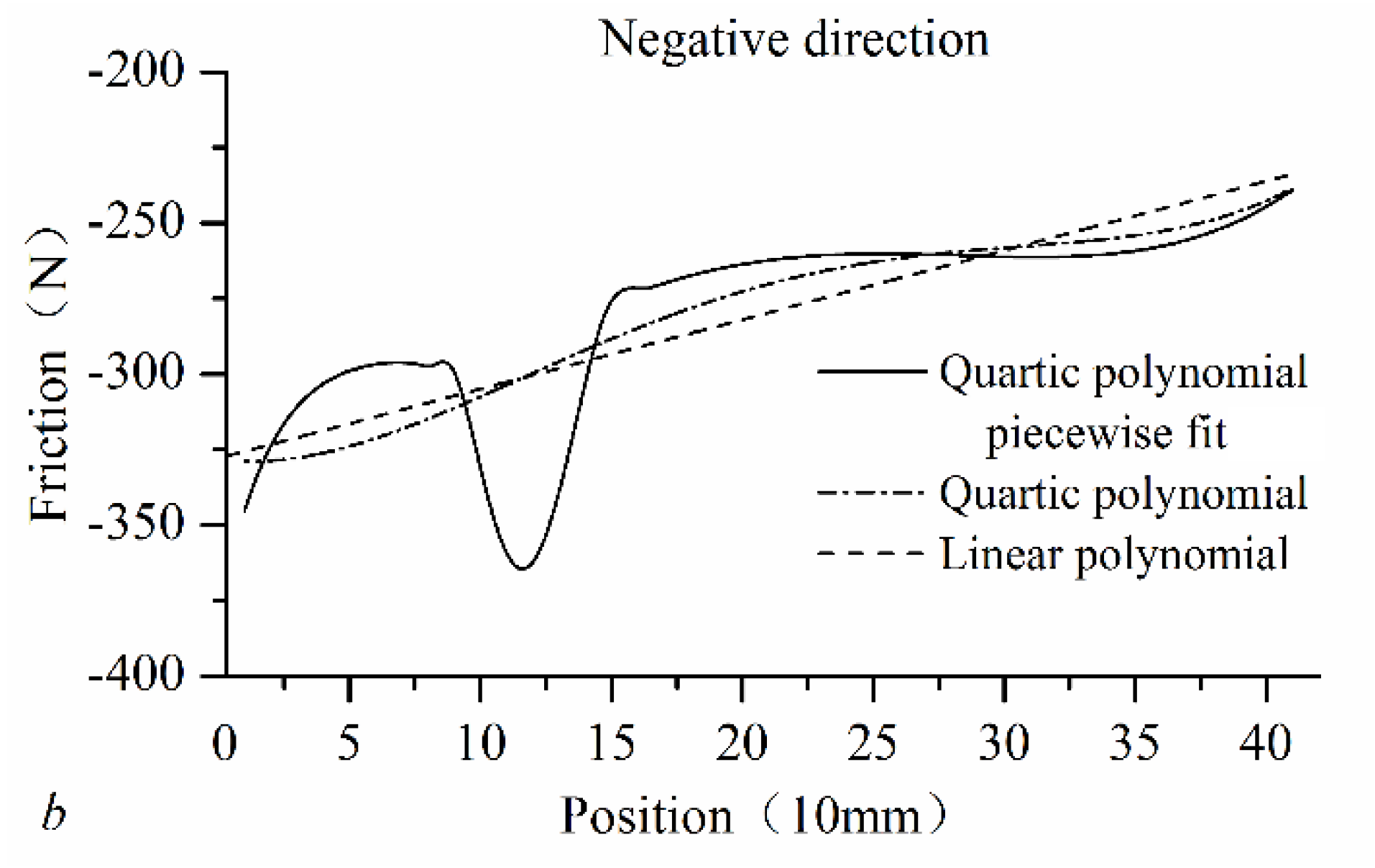
Figure 7 presents a comparison of the IAFV curves using linear, polynomial, and piecewise polynomial fits. For the linear fit, the absolute values of the IAFV increase as the worktable approaches the servomotor. The dashed-dotted lines and the solid lines fluctuate around the dashed lines. This phenomenon has been observed in studies on estimating friction [11] and on measuring the pretension in a double-nut [12]. The rigidity of the ball drive system affects the engagement of the balls and races and hence their contact forces, which causes the friction to vary. The torsional rigidity of the torque transmission segment of screw (TTSOS) decreases linearly as the distance between the worktable and the servomotor increases. The higher the torsional rigidity of the TTSOS is, the higher the contact force between the balls and the races becomes. As a result, the friction increases as the worktable approaches the servomotor.
However, incorrect alignment of the linear guides and the ball screw also results in the unbalanced spread of the inner forces [12]. An experiment was performed where a check rod, 40 mm in diameter and 400 mm in length, was installed by using the top of the lathe tailstock and the chuck. The optoNCDT 2300 sensor, which is an optical system for performing measurements with micrometer accuracy, was installed on the turret to measure the distance between the surface of the check rod and the sensor during the motion of the worktable. The worktable was set to move from 25 mm to 370 mm at a velocity of 400 mm/min. The variation in the measured distance with the position is shown in Figure 8. In Figure 8, the fluctuation curve results from the incorrect alignment of the linear guides and the ball screw. The maximum deviation A corresponds to the maximum of the IAFVs in Figure 7.
Furthermore, the lead accuracy has an impact on the inner force of the nut [12]. The difference in leads affects the engagement of the balls and races and consequently produces a variation in the friction. Due to nonuniform wear and the tolerances used in the manufacturing process of the shaft, different pitch errors were observed over the WTDOW. The experimental apparatus consists of a lathe and a servomotor installed at the end of the spindle. The turning operations are usually performed in Intervals 1 and 2, which lead to screw wear and larger pitch errors of the shaft. All of these effects determine the path of the IAFV over the WTDOW. The dashed lines in Figure 7 result from the torsional rigidity of the TTSOS, and the difference between the solid line and the dashed line results from the nonuniform pitch error and incorrect alignment of the linear guides and the ball screw. Comparing the results from Figure 5 to Figure 7 shows that the IAFVs for the forward feed are smaller than those for the backward feed, especially when the worktable approaches the servomotor. A higher friction indicates a higher force of engagement for the balls and races. The shaft is in a tensile state for the forward feed and in a compressive state for the backward feed. Thus, the shaft in a compressive state produces a higher force of engagement for the balls and races than when the shaft is in a tensile state.
4.1.2. Spectra of Friction Fluctuating Signals
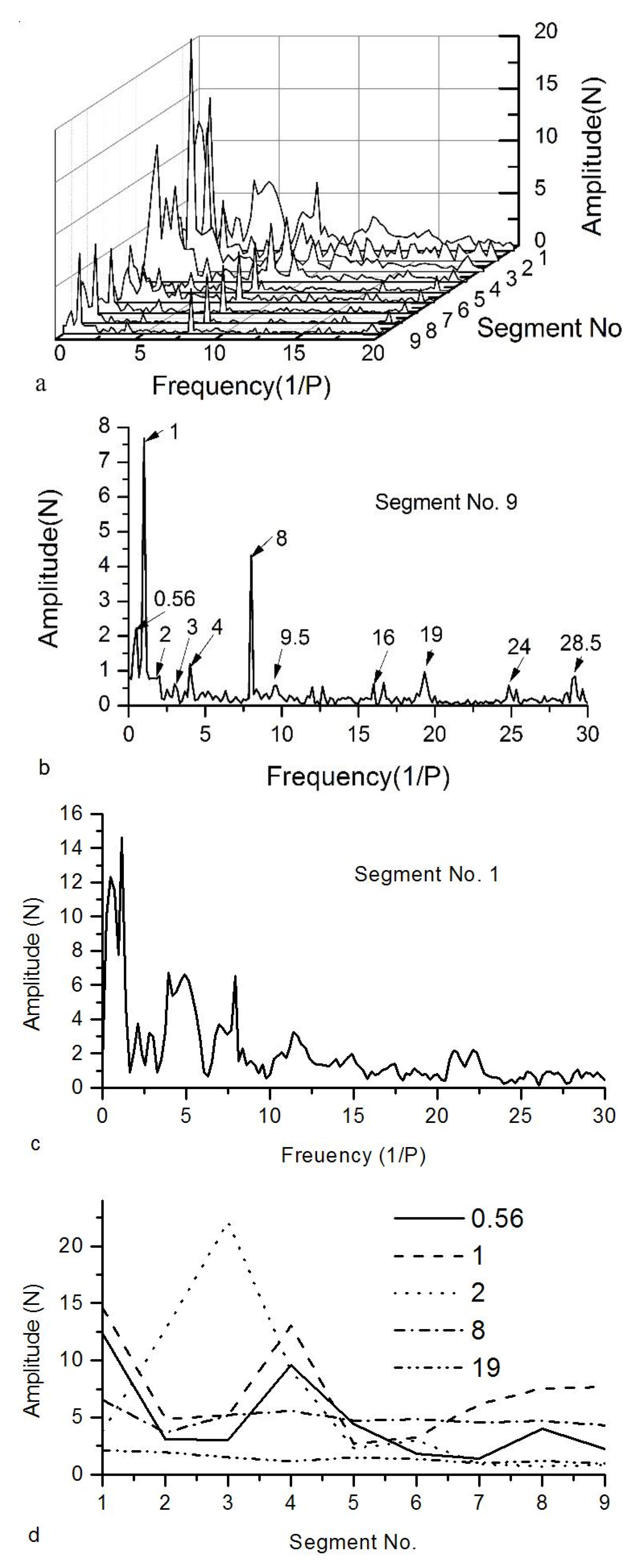
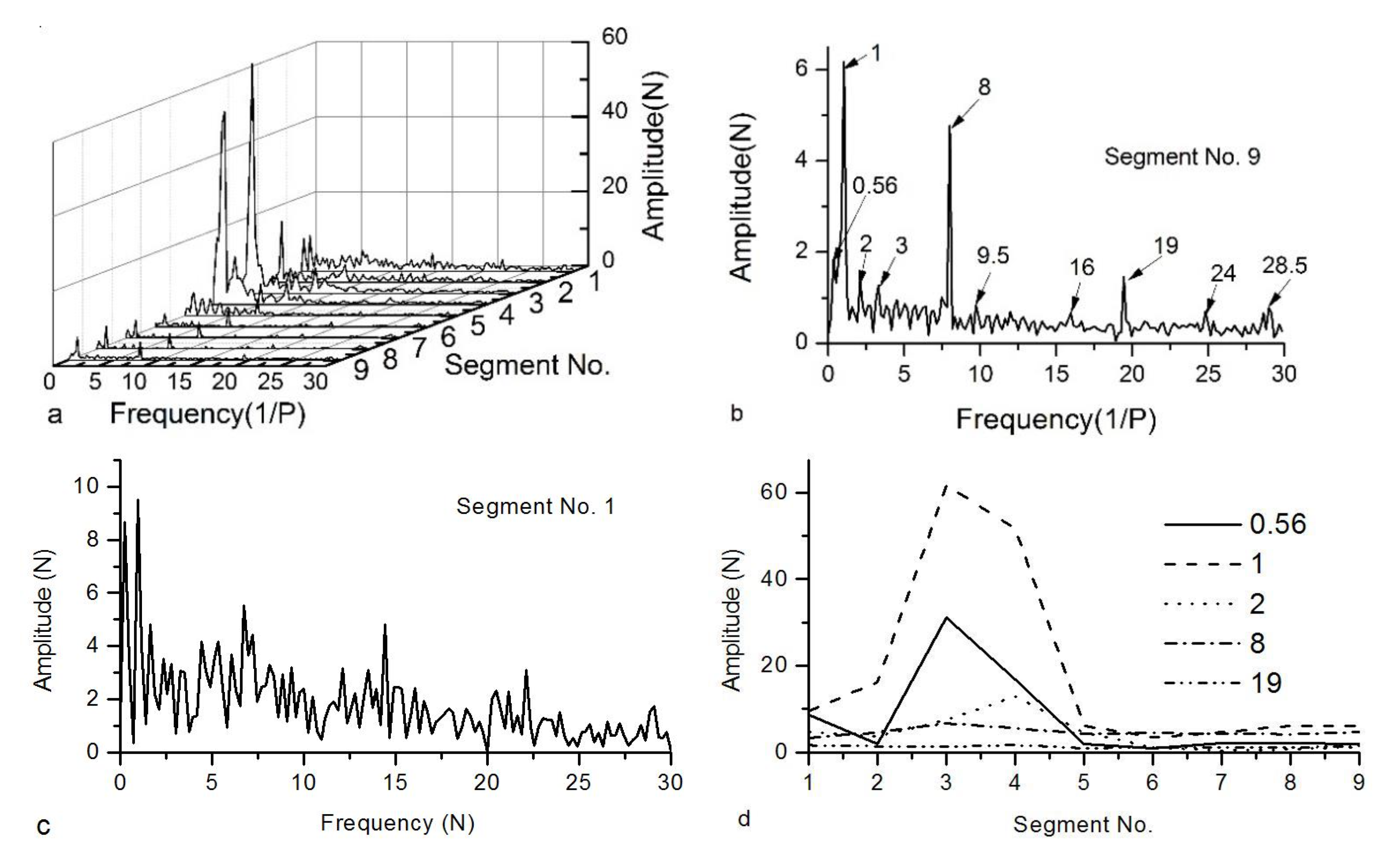
Subtracting the IAFVs plotted as solid lines of the estimated friction yields the friction fluctuating signal (FFS). To investigate the variation in the spectral characteristics of the friction with the WP, Intervals 1 and 2 are each divided into two identical segments, and Interval 3 is divided into five segments. Fast Fourier transform (FFT) is applied to the spectra to analyze the frequency characteristics of the FFS over the nine intervals. The FFT results at a feed velocity of 5 mm/min for the forward and backward feeds are shown in Figure 9 and Figure 10, respectively. As shown in Figure 9b and Figure 10b, the significant FFT components (SFFTCs) can be classified into four groups. Group 1 has only one component, 0.56; Group 2 consists of the components 1, 2, 3 and 4; Group 3 is composed of the components 8, 16, and 24; and Group 4 is composed of the components 9.5, 19 and 28.5. The amplitude of component 0.56 is attributed to the rolling tool. This component was reported in the experimental results of ball screw preloading [12]. The pitch errors of the ball screw are a significant performance index for screw manufacturing and wear in use. Variations in the leads of the screw cause nonuniform compression, resulting in an impact between the balls and races that can lead to single and multiple friction oscillations of the shaft rotating frequency, such as those observed for the amplitudes of the component in Group 2 and reported in friction studies [10] and measurements of ball and screw preloading [12]. During the motion of the feed drive servomechanism, the balls refeeding within the screw-nut and the linear ball rail guides cause an impact that leads to high frequency signals during ball and screw preloading [12,18,19]. The balls asynchronously enter and leave working circulation and slide within their recycling paths. In this way, the refeeding of the balls excites a component of the fundamental frequency as well as the components of double and triple frequencies. The fundamental frequency of the ball refeeding within the screw-nut per revolution of the shaft is expressed as
where d denotes the diameter of the lead screw; db denotes the ball diameter; β denotes the contact angle between the raceway and the ball; and z denotes the number of balls that form a circle in a raceway. For this servomechanism, .
The following values are used for the linear guide parameters in Equation (7). The diameter of the raceway of the guideway d goes to infinity; the ball diameter db is 6 mm; the contact angle β is 0; and the number of balls in the path of the raceway, z, is 19. Thus, . The amplitudes of the components for Groups 3 and 4 correspond to the friction oscillation that is excited by the refeeding of the balls within the screw-nut and the linear ball rail guides, respectively.
As shown in Figure 9a–c and Figure 10a–c, as the worktable approaches the servomotor, the amplitude spectrum of the FFS becomes more continuous, and the spectral components become more complex. These results show that the balls move more randomly within the working circulation due to the pitch errors of the shaft. As shown in Figure 9d and Figure 10d, the WP and the feed direction have very small effects on the amplitudes of components 8 and 19; they significantly affect the amplitudes of components 0.56, 1 and 2 over Intervals 1 and 2, and have small effects over Interval 3. Thus, the incorrect alignment of the linear guides and the ball screw and pitch errors can excite fluctuations in friction due to the rolling tool and the shaft lead.
4.2. Velocity-Dependent Friction Characteristics
4.2.1. Effect of the Feed Velocity on the IAFVs
In the previous section, we discussed that for a constant feed velocity, the IAFV can be expressed in terms of a piecewise polynomial fitting function of the WP. To enhance the expression accuracy of the relationship between the IAFV and the WP, three idling tests over the WTDOW were conducted to estimate the friction at one feed velocity using three groups with forward feed friction and three groups with backward feed friction. Then, a piecewise polynomial fitting algorithm was applied to the estimated friction to determine three groups of coefficients for the forward and backward feeds. The mean parameter curve method [20] was applied to the three groups of coefficients for the piecewise polynomial fits to construct new piecewise polynomials of the coefficient means (PPOCM) to describe the relationship between the mean value of instantaneous average friction (MVOIAF) and the WP. Tests were conducted for 18 specific feed velocities, ranging from 5 to 560 mm/min, to determine the relationship of the friction to the feed velocity and the WP. In Figure 11, the IAFV curves are shown for the three tests and the PPOCM curves for a feed velocity of 5 mm/min. The IAFV curves for the three tests do not coincide, except for the case of the backward feed in the interval [25, 41].
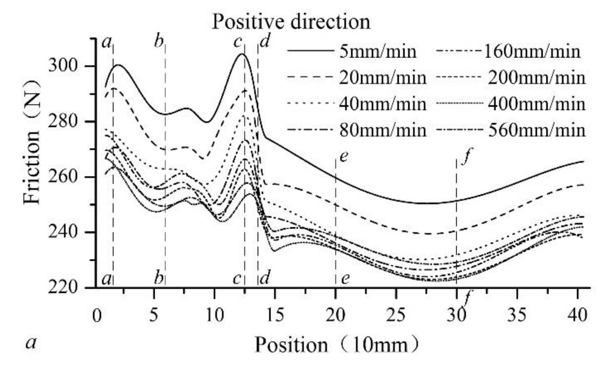
In Figure 12, the variations in the MVOIAFs with the WP are shown for eight feed velocities. For the forward feed, the MVOIAF curve exhibits its maximum at a feed velocity of 5 mm/min and a secondary maximum at a feed velocity of 20 mm/min over the WTDOW. However, the MVOIAF curves exhibit minimum values for feed velocities of 560, 400, and 200 mm/min. For the backward feed, the highest MVOIAF curve is observed for a feed velocity of 5 mm/min, except over the interval [4.9, 9.5] where there is a higher MVOIAF for a feed velocity of 20 mm/min. The MVOIAF curves exhibit minima at the following locations: over the interval [1, 9.7], at a feed velocity of 200 mm/min, over the interval [9.7, 10.05], at a feed velocity of 400 mm/min, and over the interval [10.05, 41], at a feed velocity of 560 mm/min. Therefore, the effect of feed velocity on the estimated friction varies with the WP. In addition, the peaks of the IAFV curves, which result from the pitch errors, decreases as the feed velocity increases. To describe the effect of the feed velocity on the MVOIAFs, the average coefficients of the PPOCMs are assumed to be a quintic polynomial function of the feed velocity v:
where denotes the feed direction, which is denoted by F or B for the forward or backward feeds, respectively; j denotes the interval j, where j = 1, 2, or 3;; and k denotes the kth coefficient of Equation (8), where k = 0, 1, 2, or 4.
MATLAB software was used to apply the method of least squares to the coefficients of the MVOIAF curves for the abovementioned 18 experiments to determine the coefficients of Equation (8) for the three intervals. Figure 13 is a 3D graph that shows the variations in the MVOIAF with the WP and the feed velocity. Based on the variations in the MVOIAF with the WP in Figure 12, six specific positions, denoted by a-a to f-f, were chosen to study the variation in the friction with the feed velocity. These positions are listed in Table 3.
Friction is usually expressed as a nonlinear function of velocity, such as in the Coulomb friction model, the Coulomb model with Stribeck friction, the LuGre and Leuven model, and the generalized Maxwell-slip friction model [9]. The most commonly used engineering models employ the static friction, Coulomb friction and viscous friction models. The relationship between the friction and the velocity for steady-state motion can be expressed as follows [8,21]:
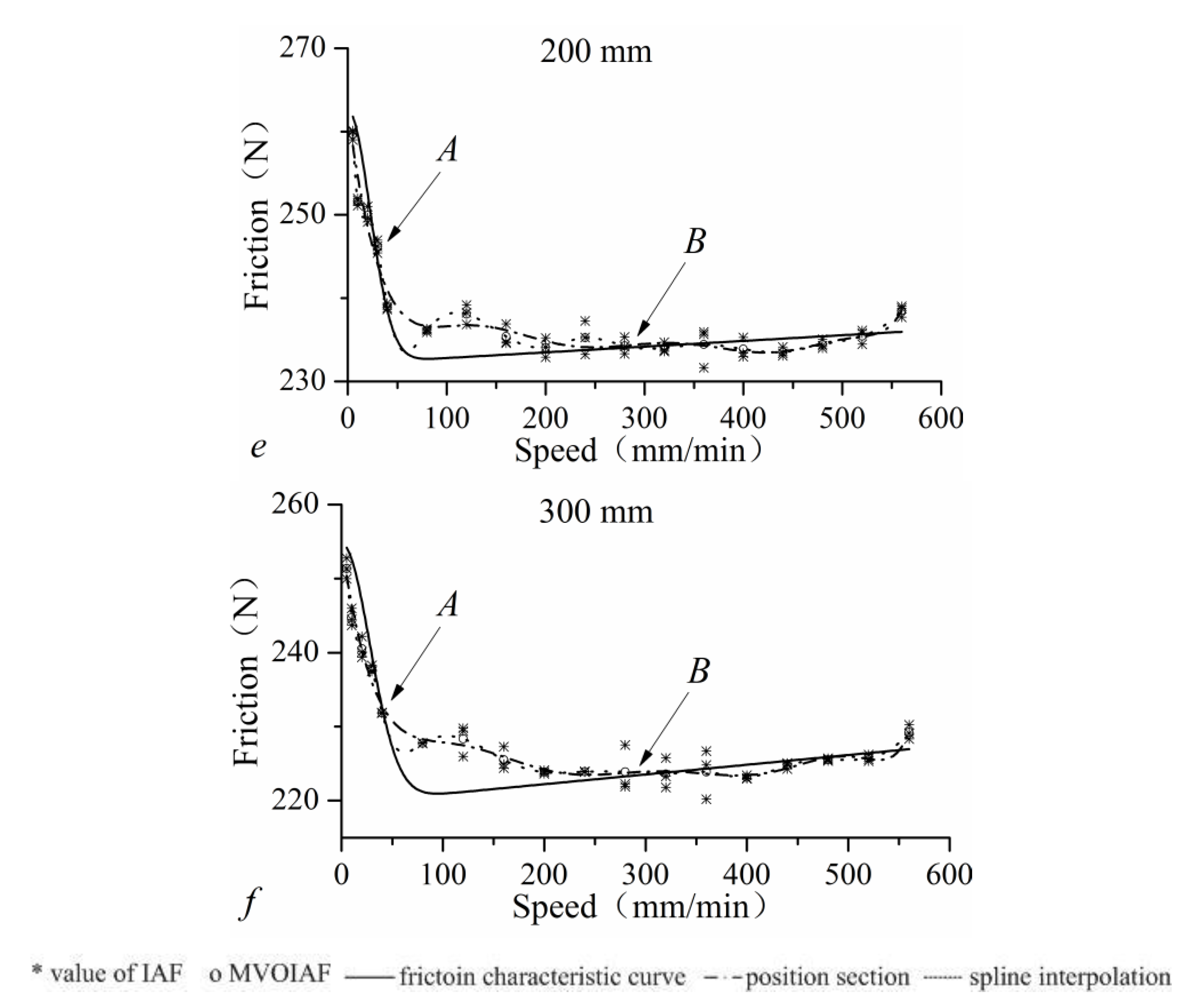
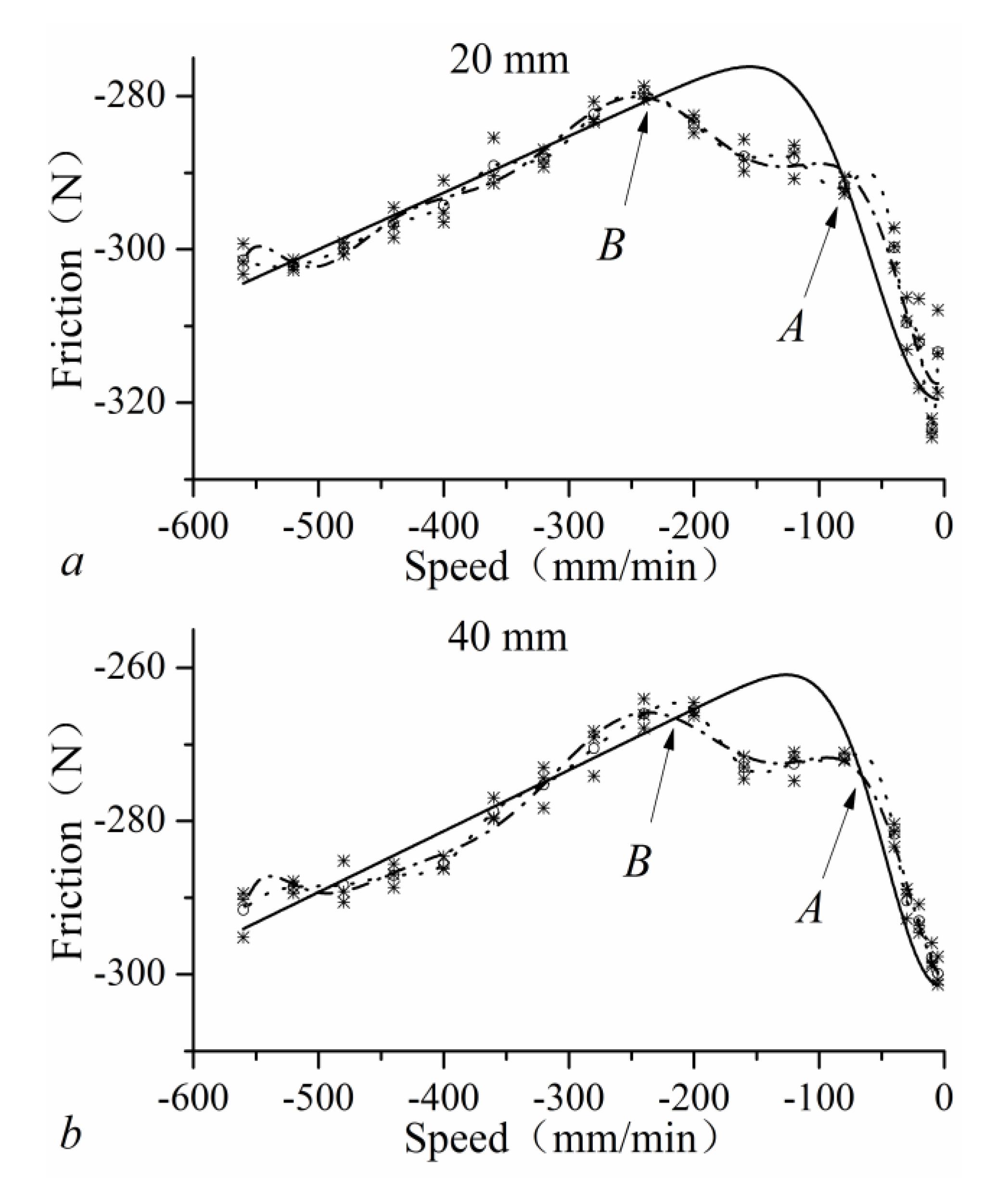
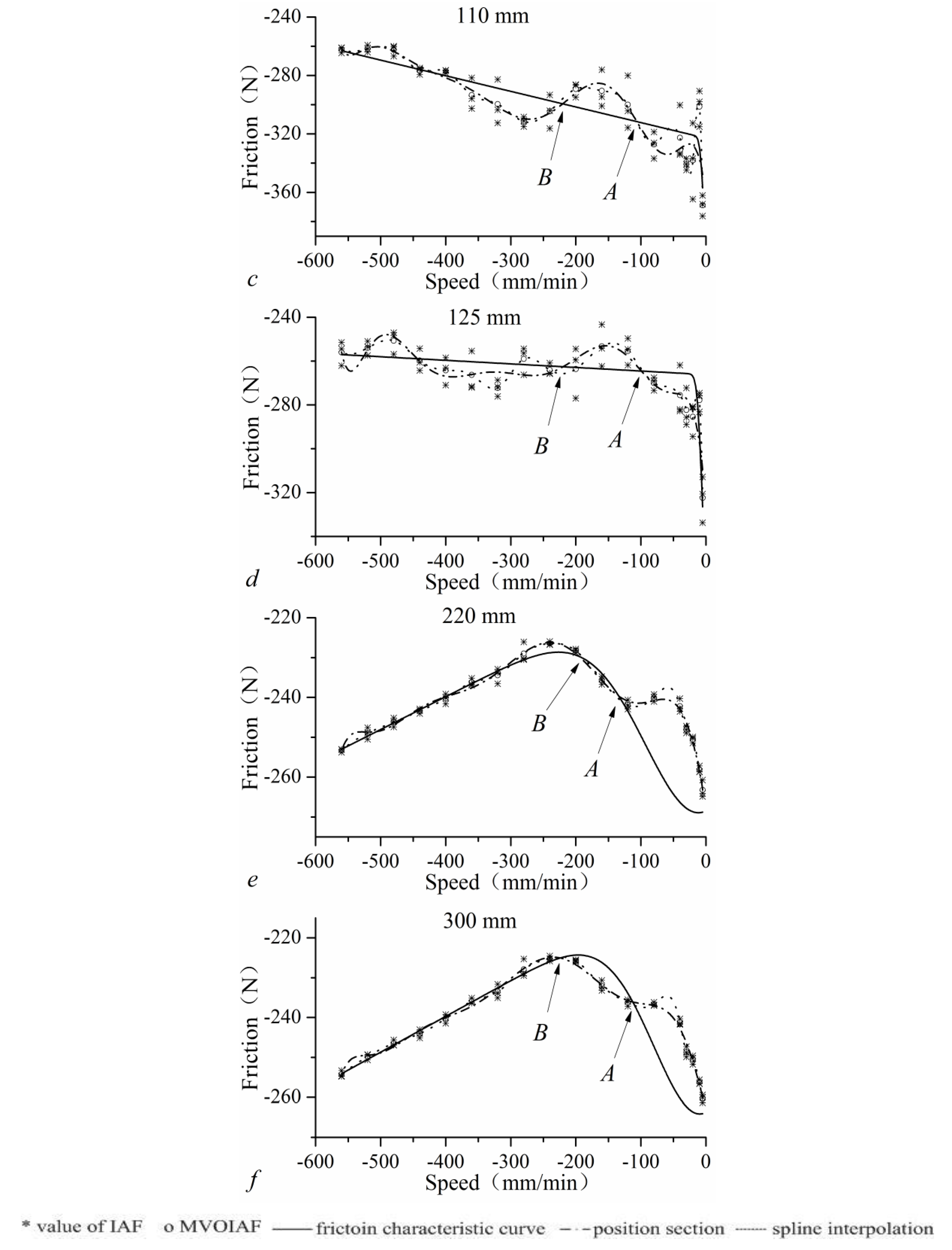
The MVOIAFs corresponding to the specific positions in Table 3 for the 18 velocities can be calculated by using the PPOCM to obtain six groups of data for the forward and backward feeds. The optimization function, fmin, which is provided by the MATLAB optimization toolbox [22], is used to identify the model parameters in Equation (9) to generate the friction characteristic curve (FCC). Figure 14 and Figure 15 provide comparisons of the experimental data with the friction characteristic curves, the position section obtained by DPFMOPV, and the spline interpolation curves of the MVOIAFs for the forward and backward feeds, respectively.
Comparing the spline interpolation curves with the position section curves in Figure 14 and Figure 15 clearly shows that the DPFMOPV can accurately predict the variations in the MVOIAFs with the WP and the feed velocity. Comparing Figure 11 and Figure 12 with Figure 14 and Figure 15 reveals that the nonuniform pitch errors of the shaft have an impact on the repeatability of the IAFVs for the three experiments. There are especially large differences during the decline following the peak of the IAF curves resulting from the pitch errors that can be observed between the three experiments in Figure 14b,d and Figure 15c,d. The IAFVs exhibit good repeatability for Interval 3 and point b-b over the range of the experimental backward feed velocity, as shown in Figure 14b,e,f. For the other intervals, the repeatability of the IAFVs is better for feed velocities above 400 mm/min. The shapes of the friction characteristic curve vary with the WP and the feed direction, and the position sections fluctuate around the corresponding friction characteristic curves. For the interval between 60 and 125 mm, the friction characteristic curves decrease as the feed velocity increases, exhibiting nonconventional Stribeck-curve behavior, as shown in Figure 14b,c and Figure 15c,d. The first two intersection points of the friction characteristic curve with the position section at the end of low feed velocity are denoted by A and B. The velocities corresponding to points A and B are denoted by and and also vary with the WP. When the feed velocity is less than , the values of the friction characteristic curve are greater than the values of the position section, and for , the values of friction characteristic curve are less than the position section values.
4.2.2. Effect of Feed Velocity on the FFS Spectra
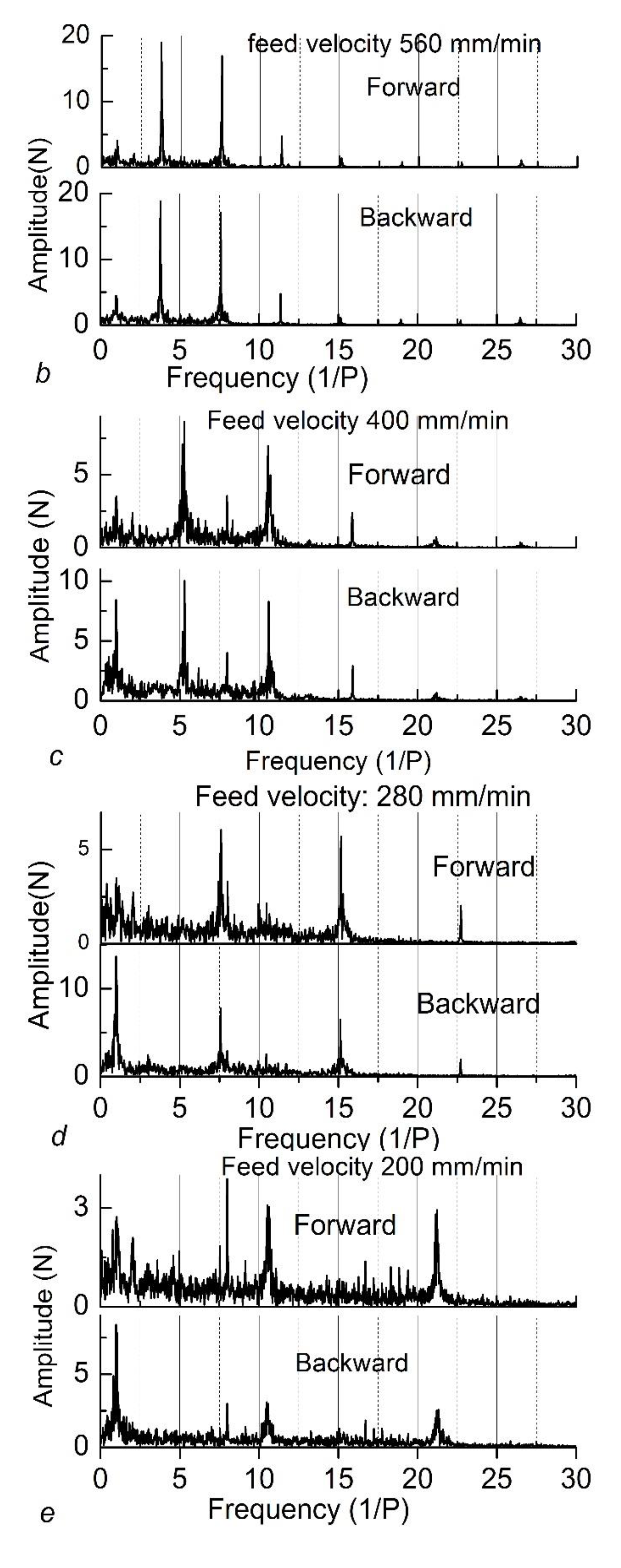
During the experimental process, the number of sampling data in one lead depends on the feed velocity. For a forward feed velocity of 560 mm/min, there are 15 data points in one lead. The component amplitudes of the FFS for the nine segments are shown in Figure 16a. There are no amplitudes of significant FFT components distributed symmetrically around 15 Hz, indicating that there is no frequency aliasing. This result verifies the effectiveness of the experimental procedure and the calculation algorithm for friction over the range of the experimental feed velocity. However, changes are observed in the frequencies of the significant components (FOSFFTC) that are greater than 3. In Figure 16b–f, the effects of the feed velocity and direction on the frequency spectrum over the WTDOW are shown. The FOSFFTCs vary with the feed velocity, but the feed direction has no effect on the FOSFFTCs.
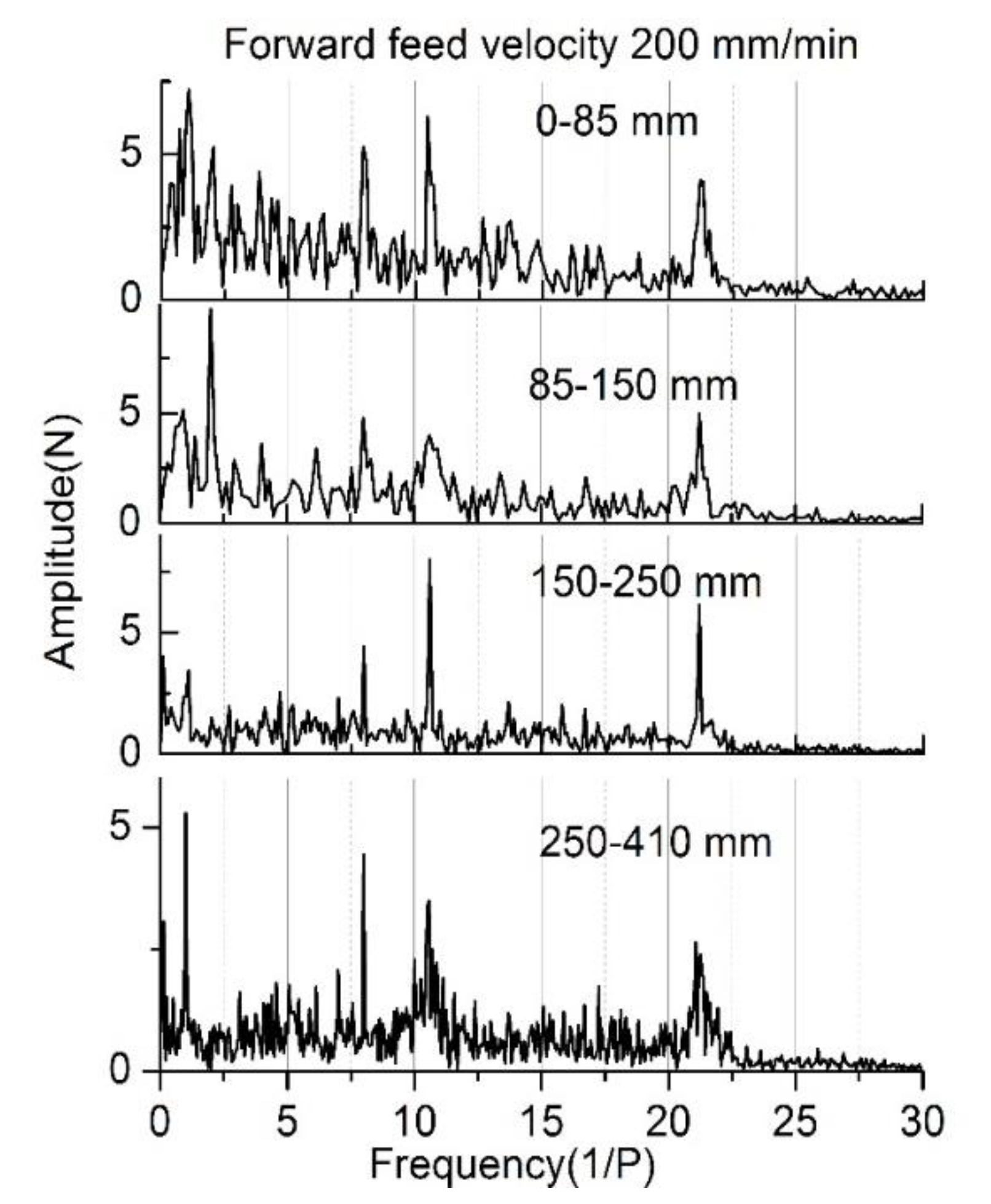
The most complex FOSFFTC in Figure 16 occurs at a forward feed velocity of 200 mm/min and is shown over different segments in Figure 17. From Figure 16 and Figure 17, it can be seen that the FOSFFTCs are constant at a fixed feed velocity. These results show that the local pitch errors have no effect on the FOSFFTCs. The balls within the working circulation of the screw-nut may undergo rolling and sliding motions. When the feed velocity is less than 120 mm/min, the balls in the screw-nut undergo pure rolling, and the FOSFFTCs are constant, as shown in Figure 9, Figure 10 and Figure 16f. However, at feed velocities above 120 mm/min, the balls experience rolling and sliding motion, which changes the refeeding frequency of the balls within the screw-nut and hence the FOSFFTCs. Therefore, change in the FOSFFTCs results from the sliding motion of the balls in the screw-nut. Here, a new frequency corresponding to the change in the FOSFFTCs is called the regenerated frequency of ball sliding motion (RFOBSM).
4.3. Discussion
The variation in the IAFV with the WP at a fixed feed velocity depends on the torsional rigidity of the TTSOS, the pitch errors, and the incorrect alignment of the linear guides and the ball screw. The higher the torsional rigidity of the TTSOS is, the higher the IAFV. Pitch errors and incorrect contact cause a local increase in the IAFV and affect the repeatability of the IAFVs for the different feed tests. The local increase in the IAFVs decreases as the feed velocity increases. The larger the nonuniform pitch errors of the shaft are, the larger the differences between the IAFVs for the different tests at low feed velocities. The variation in the MVOIAFs with the feed velocity at a fixed position exhibits nonconventional Stribeck-curve behavior.
The SFFTCs of the FFS consist of four groups. The fundamental frequency component is excited by the rolling tool marks, while the fundamental frequency and multiple components result from the pitch of the shaft and the refeeding of the balls within the screw-nut and the linear ball rail guides. At a low feed velocity, the high torsional rigidity of the TTSOS and local pitch errors cause the frequency spectrum of the FFS to become more continuous, whereas increasing the feed velocity results in discontinuities in the FFS frequency spectrum. The FOSFFTCs that are excited by the pitch of the shaft and the rolling tool marks do not vary with the feed velocity, and their amplitudes increase with the local pitch errors. The effect of local pitch errors on the amplitudes of the corresponding components decreases as the feed velocity increases. The amplitude of the fundamental frequency component resulting from the pitch of the shaft over the WTDOW for the backward feed is much greater than that for the forward feed, which is affected very little by the feed velocity. However, this difference decreases as the feed velocity increases.
The balls within the working circulation of the screw-nut undergo pure rolling for feed velocities less than 120 mm/min, rolling and intermittent sliding for feed velocities ranging from 120 to 440 mm/min, and rolling and continuous sliding for feed velocities above 440 mm/min. In pure rolling, the FOSFFTCs that are excited by the refeeding of the balls remain constant, and the amplitudes of their components are not affected by the feed velocity and direction or the WP. The direction of sliding motion is opposite to that of the ball’s center motion resulting from rolling, which produces a decrease in the fundamental frequency of the RFOBSMs. The feed direction has almost no effect on the amplitudes of the RFOBSM, which increase with the sliding velocity.
5. Conclusions
In this work, a method for estimating the friction of the servo feed system is developed by using the WP and SMTC. These are obtained from the FOCAS library function of a FANUC digital control system. A piecewise polynomial fitting algorithm is applied to the fluctuating friction patterns to separate the IAFV and the FFS. The FFT results of the FFS demonstrate that the estimated friction can effectively capture the characteristics of the frequency spectrum over the experimental range of the feed velocity.
The variations in the mean value of the IAFVs with the feed velocity for tests at a fixed WP show nonconventional Stribeck behavior. The variations in the friction force with the WP cannot be described by Stribeck characteristics. This study provides an effective method to evaluate the performance of ball screw systems and to predict friction without the use of a sensor.
Author Contributions
Conceptualization, Y.C.; Data curation, S.Z.; Formal analysis, Z.L.; Funding acquisition, C.Z.; Investigation, Y.C.; Software, Y.Z.; Writing—original draft, Y.C.; Writing—review &editing, C.Z. All authors have read and agreed to the published version of the manuscript.
Funding
This research was funded by the National Natural Science Foundation of China, grant number 51775094 and Youth Project of Liaoning Provincial Department of Education, grant number JYTQN201728.
Conflicts of Interest
The authors declare no conflict of interest.
References
- Kang, C.M.; Yu, C.; Kuo, Z.; Tie, L.; Li, J.; Yanga, B. Comprehensive compensation method for thermal error of a vertical drilling center. Trans. Can. Soc. Mech. Eng. 2019, 43, 92–101. [Google Scholar] [CrossRef] [Green Version]
- Duan, M.; Lu, H.; Zhang, X.; Zhang, Y.; Li, Z.; Liu, Q. Dynamic Modeling and Experiment Research on Twin Ball Screw Feed System Considering the Joint Stiffness. Symmetry 2018, 10, 686. [Google Scholar] [CrossRef] [Green Version]
- Yuan, W.; Fang, G.; Zhang, X.; Tang, Y.; Wan, Z.; Zhang, S. Heat Transfer and Friction Characteristics of Turbulent Flow through a Circular Tube with Ball Turbulators. Appl. Sci. 2018, 5, 776. [Google Scholar] [CrossRef] [Green Version]
- Armstrong, H.B.; Dupont, P.; Canudasde Wit, C.A. Survey of models, analysis tools and compensation methods for the control of machines with friction. Automatic 1994, 30, 1083–1138. [Google Scholar] [CrossRef]
- Lampacrt, V.; Al-bender, F.; Swevers, J. The generalized maxwell-slip friction model: A novel model for friction simulation and compensation. IEEE Trans. Autom. Control 2005, 50, 1883–1887. [Google Scholar] [CrossRef]
- Karnopp, D. Computer simulation of stick-slip friction in mechanical dynamic systems. Asme J. Dyn. Sys. Meas. Contr. 1985, 107, 100–103. [Google Scholar] [CrossRef]
- Xua, N.; Tanga, W.; Chena, Y.; Baoa, D.; Guob, Y. Modeling analysis and experimental study for the fiction of a ball screw. Mech. Mach. Theory 2015, 87, 57–69. [Google Scholar] [CrossRef]
- Caudasde Wit, C.A.; Olsson, H.; Astrom, K.J. A new model for control of systems with friction. IEEE Trans. Auto. Contr. 1995, 40, 419–425. [Google Scholar] [CrossRef] [Green Version]
- Tjahjowidodo, T.; Al-Bender, F.; Van Brussel, H.; Symens, W. Friction characterization and compensation in electro-mechanical systems. J. Sound. Vib. 2007, 308, 632–646. [Google Scholar] [CrossRef]
- Yeh, S.S.; Su, H.C. Development of friction identification methods for feed drives of CNC machine tools. Int. J. Manuf. Technol. 2011, 52, 263–278. [Google Scholar] [CrossRef]
- Yamada, Y.; Kakinuma, Y. Sensorless cutting force estimation for full-closed controlled ball-screw-driven stage. Int. J. Adv. Manuf. Technol. 2016, 87, 3337–3348. [Google Scholar] [CrossRef]
- Frey, S.; Walther, M.; Verl, A. Periodic variation of preloading in ball screws. Prod. Eng. Res. Devel. 2010, 4, 261–267. [Google Scholar] [CrossRef]
- FANUC, FOCAS1: FANUC Open CNC API Sepcifications version 1-FOCAS1/Ethernet CNC/PMC Data window library. 2003. Available online: http://www.graco.unb.br/alvares/romi/Focas1/Disk2/Doc/FWLIB32.htm (accessed on 1 January 2016).
- Álvares, A.J.; Ferreira, J.C.E. WebTurning: Teleoperation of a CNC turning center through the Internet. J. Mater. Process. Technol. 2006, 179, 251–259. [Google Scholar] [CrossRef]
- Satito, K.; Kamiyama, K.; Ohmea, T.; Matsuda, T. A microprocessor-controlled speed regulator with instantaneous speed estimation for motor drives. IEEE Trans. Ind. Electron. 1988, 35, 95–99. [Google Scholar] [CrossRef]
- Brown, R.H.; Sechneider, S.C.; Mulligan, M.G. Analysis of algorithms for velocity estimation from discrete position versus time data. IEEE Trans. Ind. Electron. 1992, 39, 11–19. [Google Scholar] [CrossRef]
- Hou, C.J.; Ceng, Y.S.; Wu, D.Q. Global Continuous Curve Fitting Method of Piecewise Least Square Fitting with Global Continuity. J. Chongqing Norm. Univ. (Nat. Sci.) 2011, 28, 44–48. [Google Scholar]
- Hung, J.P.; James, S.S.; Jerry, J. Impact failure analysis of re-circulating mechanism in ball serew. Eng. Fail. Anal. 2004, 11, 561–573. [Google Scholar] [CrossRef]
- Ispaylar, M.H. Betriebseigenschafen von Profilschienen Wälzführungen; CompuTEAM: Somerset, UK, 1996; pp. 116–124. [Google Scholar]
- Liu, Q. The differences between the mean of fluorescence parameter and parameter value of average curve of fast chlorophyll a fluorescence induction curves. For. Sci. Technol. 2015, 40, 10–14. [Google Scholar]
- Xi, X.C.; Poo, A.N.; Hong, G.S. Tacking error-based static friction compensation for a bi-axial CNC machine. Precis. Eng. 2010, 480–488. [Google Scholar] [CrossRef]
- Grace, A. Optimization Toolbox for Use with MATLAB User’s Guide; The MathWorks Inc.: Natick, MA, USA, 1994. [Google Scholar] [CrossRef]
Figure 1.
Experimental setup.

Figure 2.
The API FOCAS1 protocol.
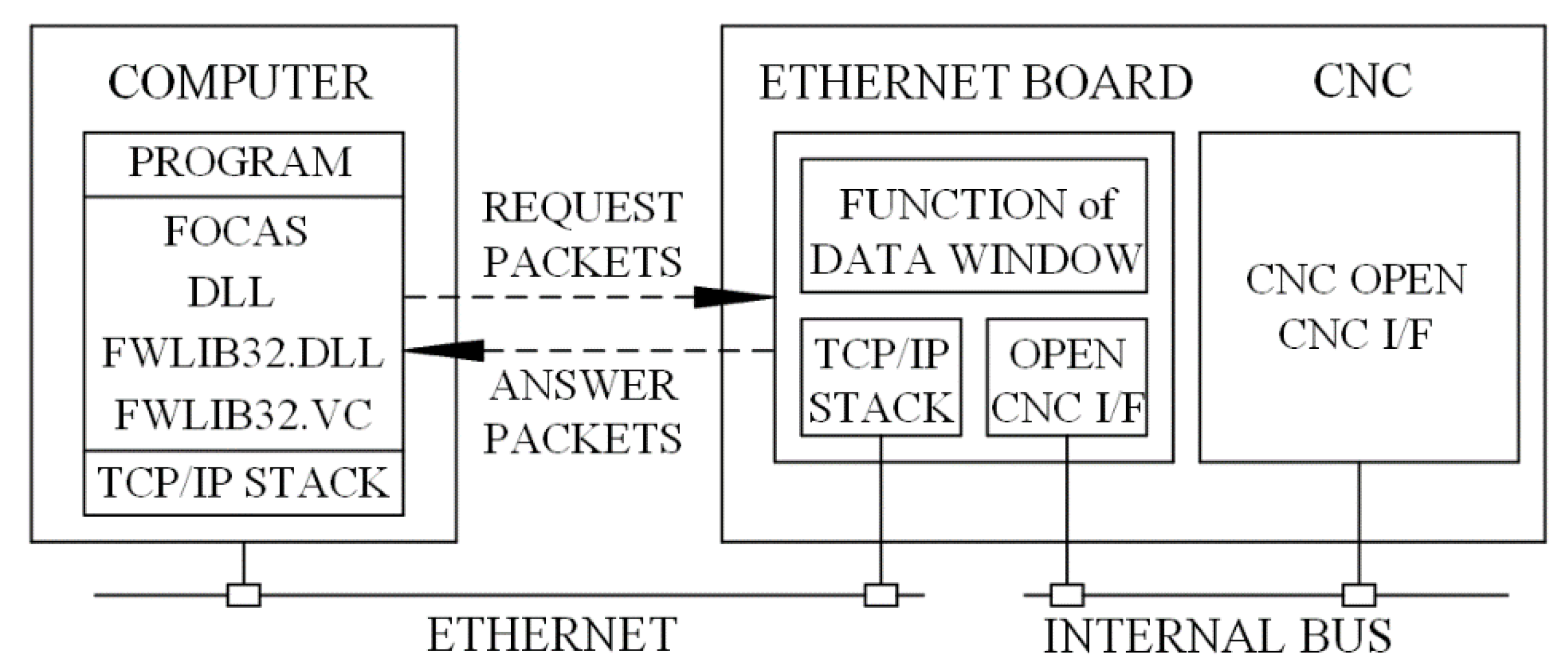
Figure 3.
Block diagram of the data collection application program.

Figure 4.
Servo feed drive system for a lathe along the z-axis.
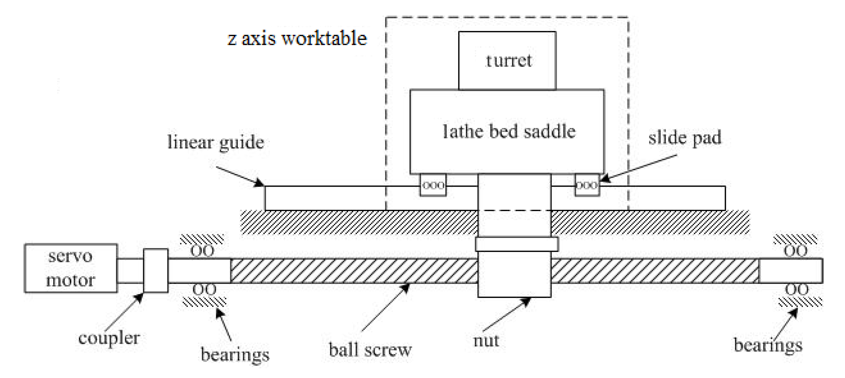
Figure 5.
Variation in the estimated friction with WP for a feed velocity of 5 mm/min.
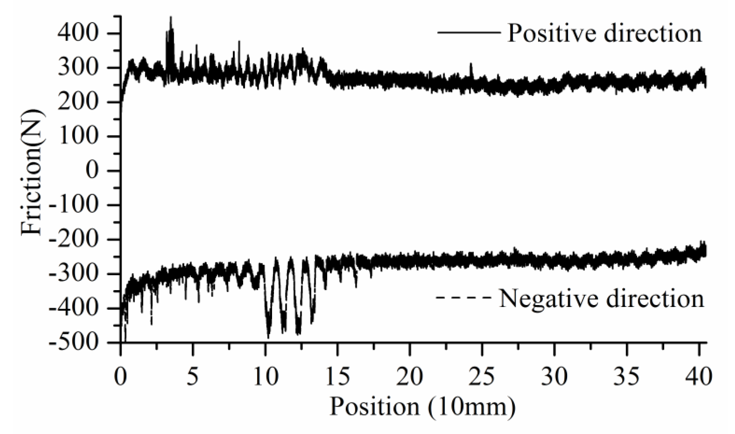
Figure 6.
Comparison of the estimated friction with IAFVs. (a) Position direction; (b) Negative direction.
Figure 6.
Comparison of the estimated friction with IAFVs. (a) Position direction; (b) Negative direction.
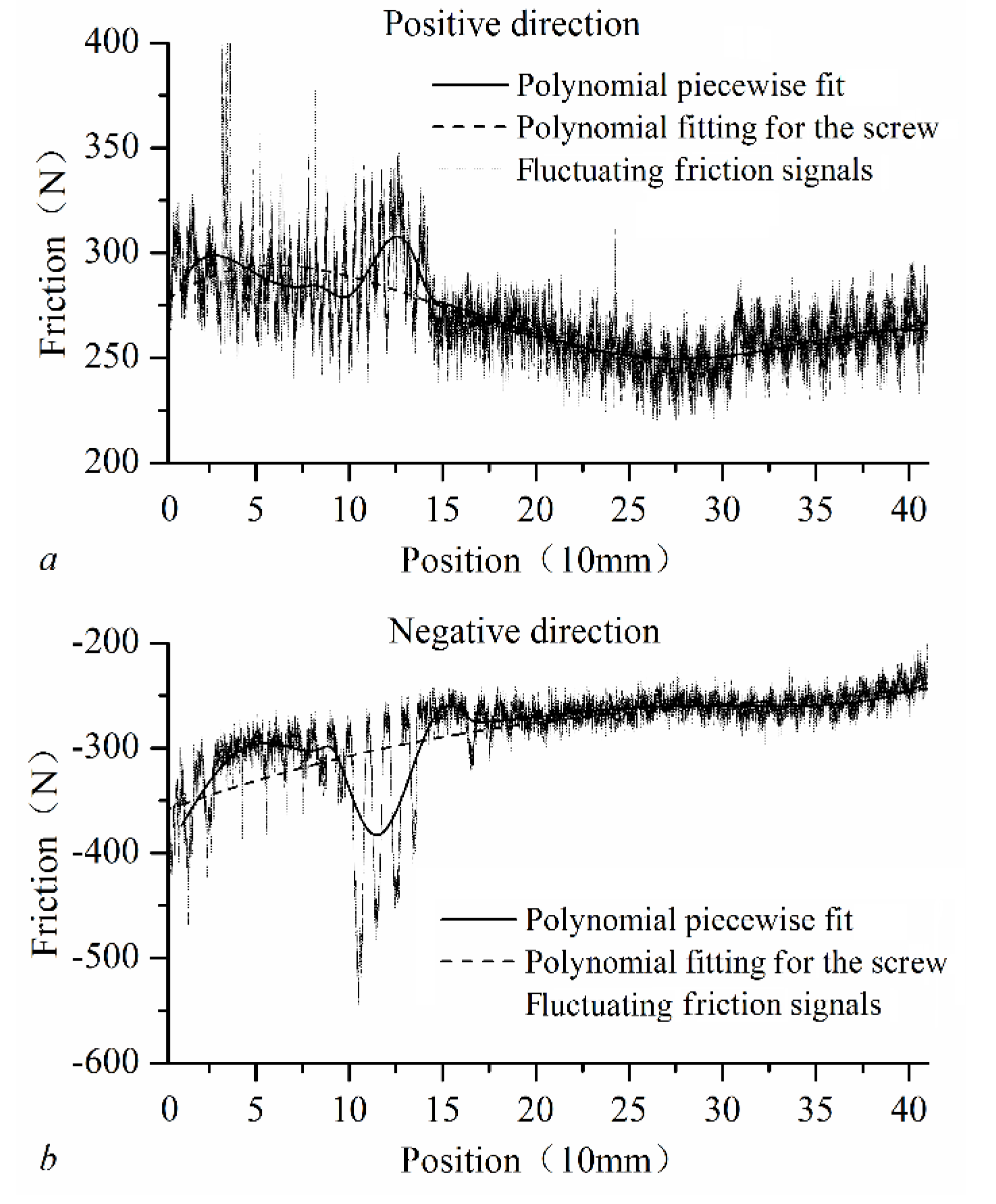
Figure 7.
IAFVs obtained using linear, quartic, and piecewise polynomial fits. (a) Position direction; (b) Negative direction.
Figure 7.
IAFVs obtained using linear, quartic, and piecewise polynomial fits. (a) Position direction; (b) Negative direction.
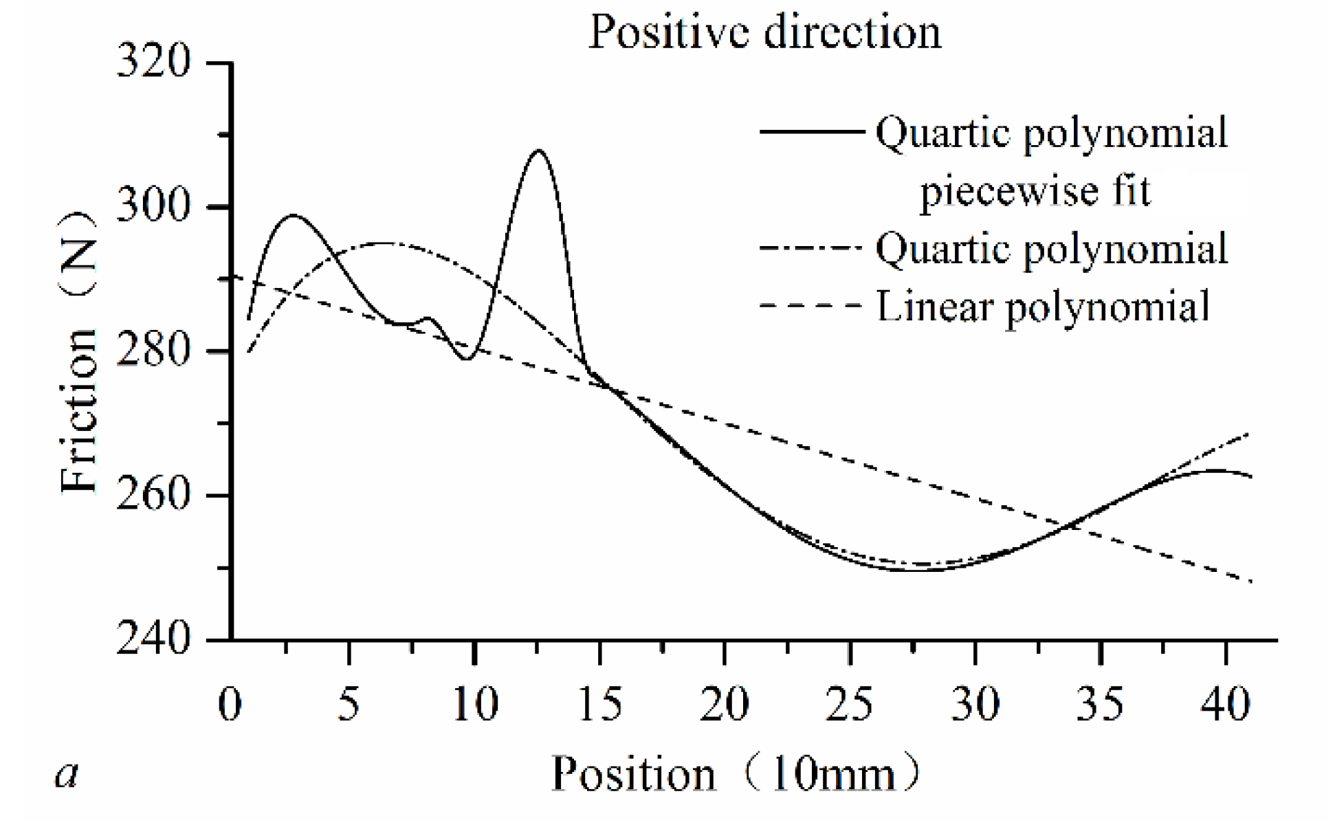

Figure 8.
Variation in the measured distance with WP.
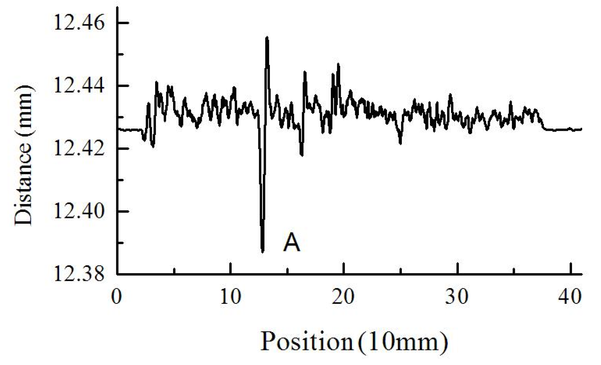
Figure 9.
Variations in the friction frequency spectrum with WP at a forward feed of 5 mm/min. (a) FFS of all segments; (b) FFS of segment No. 9; (c) FFS of segment No. 1; (d) Amplitude of all segments for significant frequency components.
Figure 9.
Variations in the friction frequency spectrum with WP at a forward feed of 5 mm/min. (a) FFS of all segments; (b) FFS of segment No. 9; (c) FFS of segment No. 1; (d) Amplitude of all segments for significant frequency components.

Figure 10.
Variations in the friction frequency spectrum with the WP at a backward feed of 5 mm/min. (a) Friction frequency spectrum of all the segments; (b) Friction frequency spectrum of segment No. 9; (c) Friction frequency spectrum of segment No. 1; (d) Amplitude of all segments for significant frequency components.

Figure 11.
IAFV curves and associated MVOIAF for three tests at a feed velocity of 5 mm/min. (a) Position direction; (b) Negative direction.
Figure 11.
IAFV curves and associated MVOIAF for three tests at a feed velocity of 5 mm/min. (a) Position direction; (b) Negative direction.

Figure 12.
Variations in the MVOIAF with WP for the different feed velocities. (a) Position direction; (b) Negative direction.
Figure 12.
Variations in the MVOIAF with WP for the different feed velocities. (a) Position direction; (b) Negative direction.

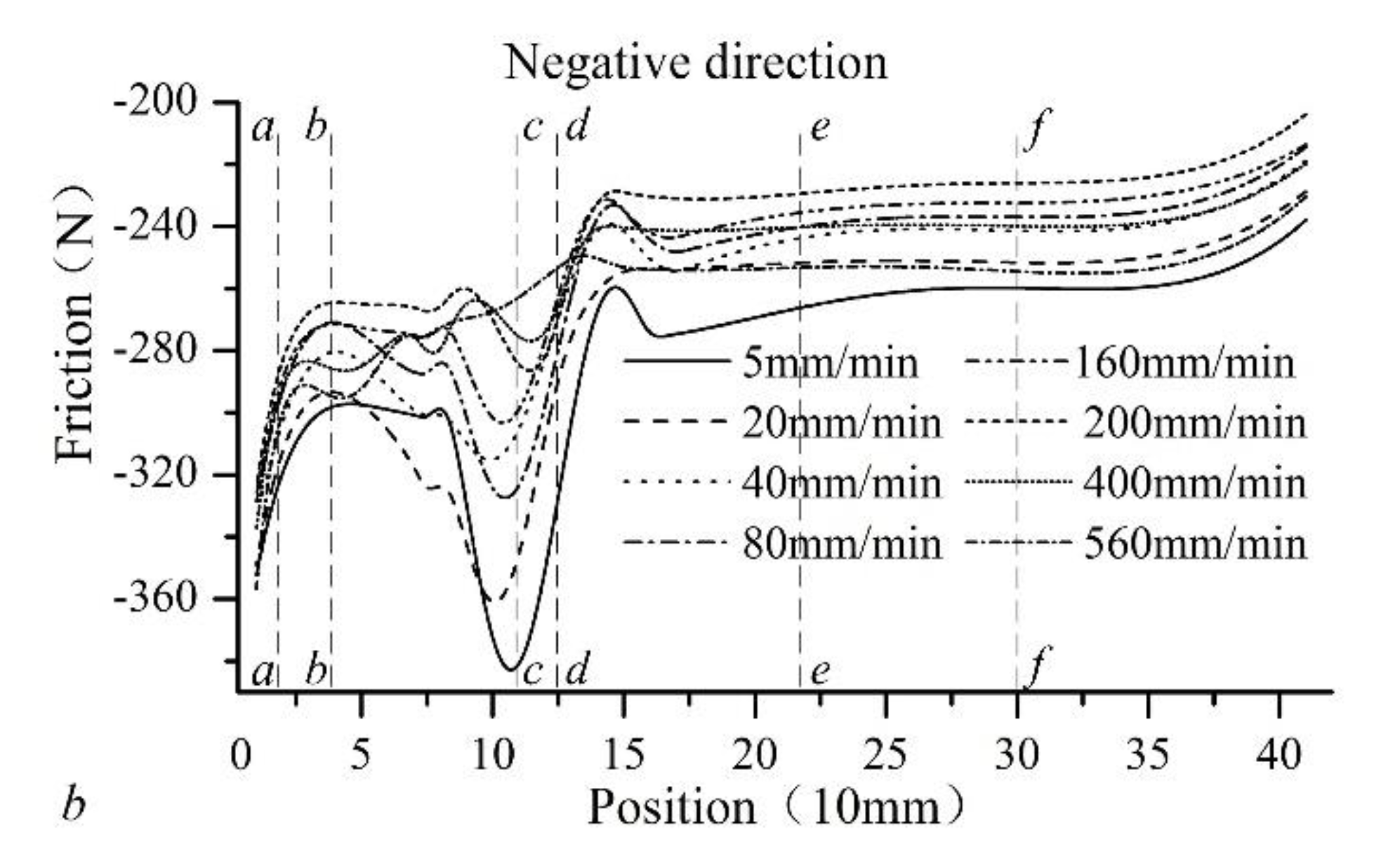
Figure 13.
Variations in the MVOIAF with WP and the feed velocity.
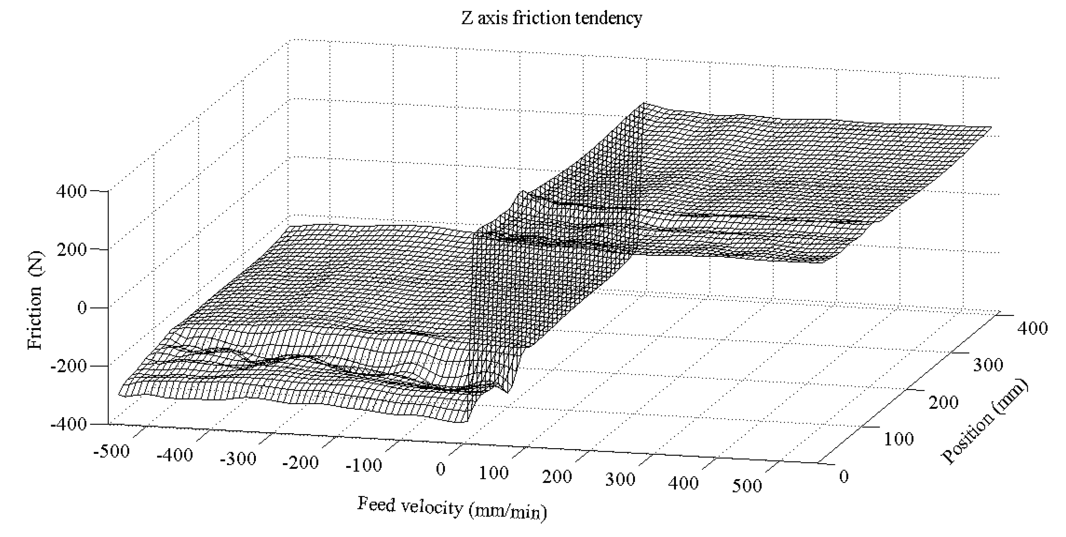
Figure 14.
Comparison of the experimental data with three model curves for the forward feed. (a) Position of 20 mm; (b) Position of 60 mm; (c) Position of 125 mm; (d) Position of 135 mm; (e) Position of 200 mm; (f) Position of 300 mm.
Figure 14.
Comparison of the experimental data with three model curves for the forward feed. (a) Position of 20 mm; (b) Position of 60 mm; (c) Position of 125 mm; (d) Position of 135 mm; (e) Position of 200 mm; (f) Position of 300 mm.
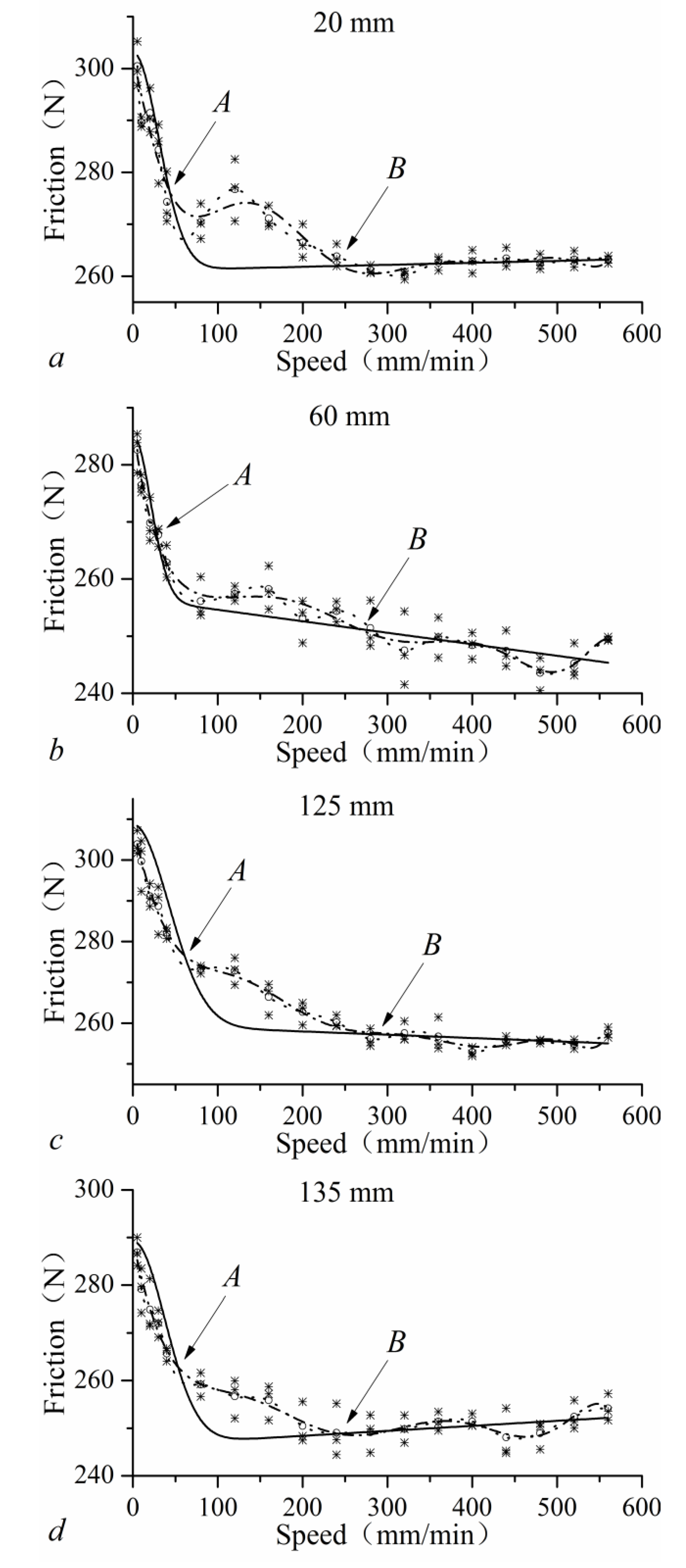

Figure 15.
Comparison of the experimental data with three model curves for the backward feed. (a) Position of 20 mm; (b) Position of 40 mm; (c) Position of 110 mm; (d) Position of 125 mm; (e) Position of 220 mm; (f) Position of 300 mm.
Figure 15.
Comparison of the experimental data with three model curves for the backward feed. (a) Position of 20 mm; (b) Position of 40 mm; (c) Position of 110 mm; (d) Position of 125 mm; (e) Position of 220 mm; (f) Position of 300 mm.


Figure 16.
Effects of the feed velocity and direction on the FFT spectrum for FFS. (a) The component amplitudes of the FFS for the nine segments at the forward feed velocity of 560 mm/min; (b) The frequency spectrum over the WTDOW at the feed velocity of 560 mm/min; (c) The frequency spectrum over the WTDOW at the feed velocity of 400 mm/min; (d) The frequency spectrum over the WTDOW at the feed velocity of 280 mm/min; (e) The frequency spectrum over the WTDOW at the feed velocity of 200 mm/min; (f) The frequency spectrum over the WTDOW at the feed velocity of 80 mm/min.
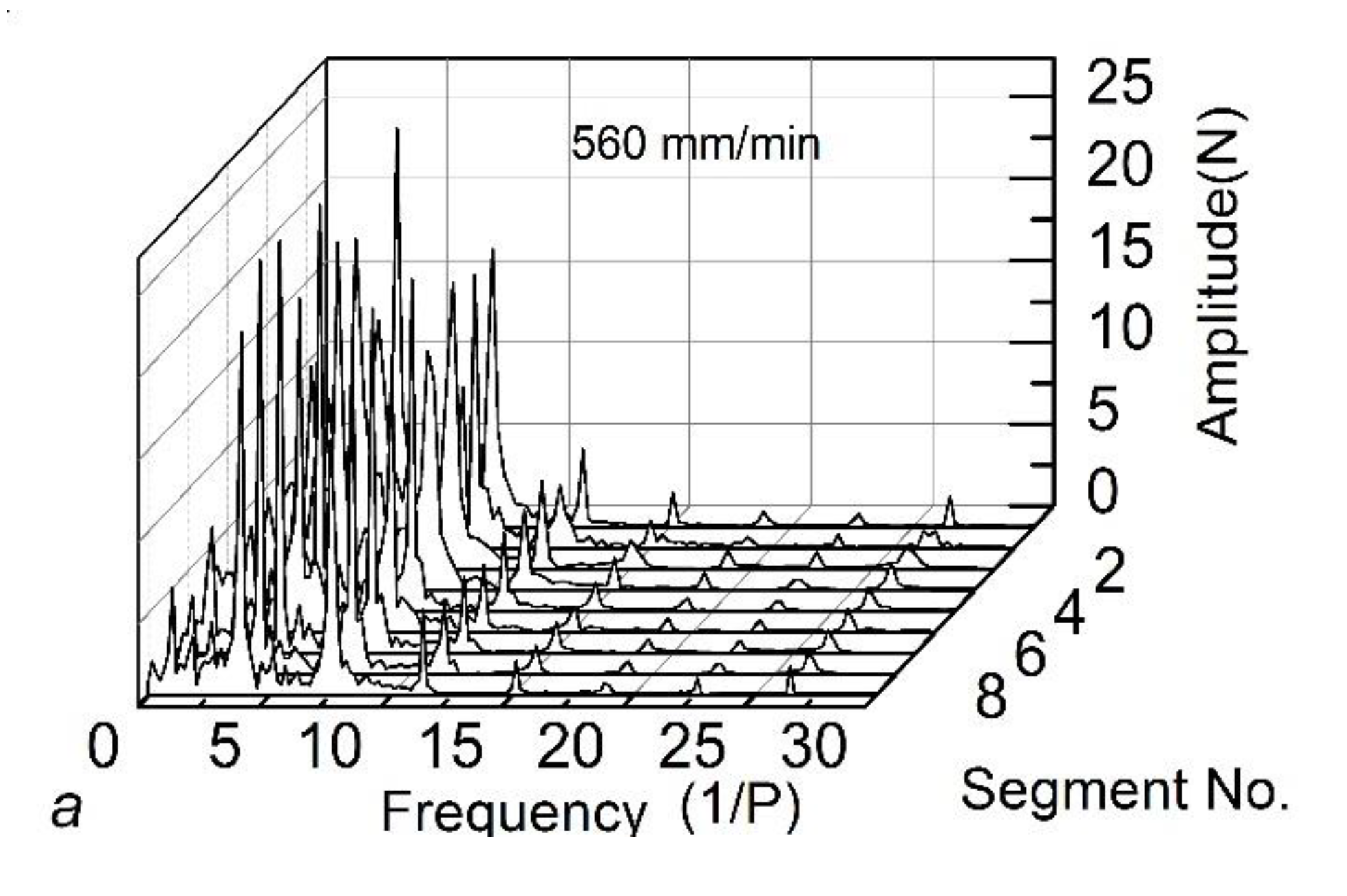

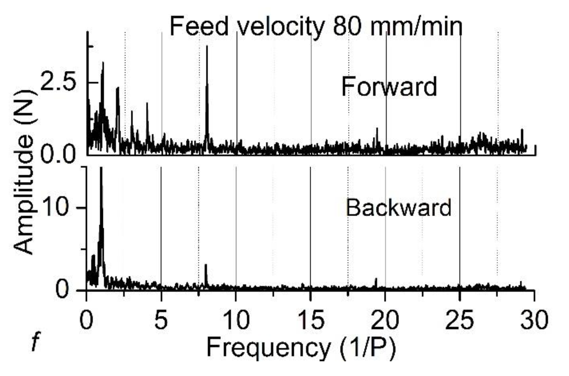
Figure 17.
Amplitudes of FFT components for different segments.

Table 1.
Specifications for the ball screw drive system.
| Parameters | Value | Unit | |
|---|---|---|---|
| Lathe | Worktable mass | 425 | kg |
| Screw lead | 10 | mm | |
| Ball diameter of lead screw | 5.56 | mm | |
| Ball diameter of linear guideway | 5.56 | mm | |
| Number of balls for the guideway in a raceway | 19 | ||
| Return position Z0 | 410 | mm | |
| Return position Z1 | 0 | mm | |
| Servomotor | Type | β12/3000is | |
| Torque coefficient | 1.82 | Nm/A |
Table 2.
Values of standard deviation for different order polynomial fits.
| Order | 1 | 2 | 3 | 4 | 5 | 6 |
|---|---|---|---|---|---|---|
| Positive | 19.1 | 18.4 | 17.1 | 16.8 | 17.0 | 17.5 |
| Negative | 31.8 | 30.6 | 30.0 | 29.65 | 31.2 | 29. 6 |
Table 3.
Position corresponding to the symbols a-a to f-f in Figure 12.
Table 3.
Position corresponding to the symbols a-a to f-f in Figure 12.
| Symbol | a-a | b-b | c-c | d-d | e-e | f-f |
|---|---|---|---|---|---|---|
| Positive (mm) | 20 | 60 | 125 | 135 | 200 | 300 |
| Negative (mm) | 20 | 40 | 110 | 125 | 220 | 300 |
© 2020 by the authors. Licensee MDPI, Basel, Switzerland. This article is an open access article distributed under the terms and conditions of the Creative Commons Attribution (CC BY) license (http://creativecommons.org/licenses/by/4.0/).
Share and Cite
MDPI and ACS Style
Chen, Y.; Zhang, S.; Zhang, Y.; Lu, Z.; Zhao, C. Investigation on Sensorless Estimating Method and Characteristics of Friction for Ball Screw System. Appl. Sci. 2020, 10, 3122. https://doi.org/10.3390/app10093122
AMA Style
Chen Y, Zhang S, Zhang Y, Lu Z, Zhao C. Investigation on Sensorless Estimating Method and Characteristics of Friction for Ball Screw System. Applied Sciences. 2020; 10(9):3122. https://doi.org/10.3390/app10093122
Chicago/Turabian StyleChen, Ye, Siyu Zhang, Yanzhou Zhang, Zechen Lu, and Chunyu Zhao. 2020. "Investigation on Sensorless Estimating Method and Characteristics of Friction for Ball Screw System" Applied Sciences 10, no. 9: 3122. https://doi.org/10.3390/app10093122
Note that from the first issue of 2016, this journal uses article numbers instead of page numbers. See further details here.