Article

Fast Simulation of Laser Heating Processes on Thin Metal Plates with FFT Using CPU/GPU Hardware

1
Vicomtech Foundation, Basque Research and Technology Alliance (BRTA), Mikeletegi 57, 20009 San Sebastián, Spain
2
Laboratory of CAD CAM CAE, Universidad EAFIT, Cra 49 no 7-sur-50, Medellín 050022, Colombia
3
High Performance Computing Facility APOLO, Universidad EAFIT, Cra 49 no 7-sur-50, Medellín 050022, Colombia
*
Author to whom correspondence should be addressed.
Appl. Sci. 2020, 10(9), 3281; https://doi.org/10.3390/app10093281
Submission received: 23 March 2020 / Revised: 18 April 2020 / Accepted: 1 May 2020 / Published: 8 May 2020

Abstract

:
In flexible manufacturing systems, fast feedback from simulation solutions is required for effective tool path planning and parameter optimization. In the particular sub-domain of laser heating/cutting of thin rectangular plates, current state-of-the-art methods include frequency-domain (spectral) analytic solutions that greatly reduce the required computational time in comparison to industry standard finite element based approaches. However, these spectral solutions have not been presented previously in terms of Fourier methods and Fast Fourier Transform (FFT) implementations. This manuscript presents four different schemes that translate the problem of laser heating of rectangular plates into equivalent FFT problems. The presented schemes make use of the FFT algorithm to reduce the computational time complexity of the problem from O ( M 2 N 2 ) to O ( M N log ( M N ) ) (with M × N being the discretization size of the plate). The test results show that the implemented schemes outperform previous non-FFT approaches both in CPU and GPU hardware, resulting in 100 × faster runs. Future work addresses thermal/stress analysis, non-rectangular geometries and non-linear interactions (such as material melting/ablation, convection and radiation heat transfer).

1. Introduction

Based on virtual modelling and simulation of physical phenomena, Industry 4.0 solutions aim to integrate interactive virtual worlds with their equivalent physical part (e.g., using digital twins). These solutions enable the development of decision making tools that can be of great use in the optimization of manufacturing processes.
In this context, engineering solutions use extensively Finite Element Analysis (FEA) for simulation of such physical phenomena (e.g., acoustics, heat transfer, structural analysis, fluid flow, etc.). However, FEA approaches require a great amount of computation resources. In contrast, spectral analysis and spectral methods are competitive alternatives to numerical simulations. These methods provide frequency-domain solutions (infinite sum of trigonometric functions) to the Partial Difference Equations (PDEs) that model such physical phenomena.
In the particular sub-domain of laser heating/cutting simulation, frequency-based algorithms have been developed for heat transfer analysis on rectangular plates. These algorithms are faster than traditional numerical methods (such as Finite Element Methods) at the cost of some model simplifications. In addition, these methods provide some advantages over FEA, such as allowing to zoom into asynchronous time intervals without computing or storing the complete history of the solution.
This property makes frequency-based algorithms more adequate for decision making tools that require rapid response times, allowing to be more flexible towards changes in the heating/cutting manufacturing process. Fast simulation of the laser heating/cutting problem is very important for different engineering problems, such as tool path planning, laser parameter optimization, waste and resources optimization, and so forth. Moreover, interactive simulation and visualization of laser machining processes contributes to many different challenges and opportunities currently present in the Industry 4.0 framework [1].
The aforementioned methods for laser heating/cutting simulation allow simulation of complex laser trajectories on rectangular plates, including parametric trajectories and the introduction of multiple laser beams simultaneously. However, there are no Fast Fourier Transform (FFT)-based solutions to the laser heating/cutting problem in the current state of the art.
The FFT is a widely used algorithm not only in the context of PDEs simulation, but also in other areas such as signal analysis and image processing. Thus, its development has been refined and studied extensively in the literature. Several FFT algorithms exist in the literature that further optimize the computation in function of the input signal properties (e.g., symmetry, real/imaginary, size, etc.). In general, the FFT is a key algorithm that retrieves the original spatial-based solution by performing a factorization of the Discrete Fourier Transform (DFT) and avoids redundant computations, reducing the computational complexity of the original DFT problem [2].
This article presents four different schemes that cast the laser heating/cutting problem into DST (Discrete Sine Transform) and DFT (Discrete Fourier Transform) problems. Such casting enables the use of FFT libraries to implement these schemes. The test results show a significant improvement over existing methods in the computational time, both in CPU and GPU, due to the computational complexity reduction.
This manuscript is an extension of the work presented in Reference [3], where only two schemes were briefly introduced for the FFT computation of the laser heating problem. The current research discusses in more detail each of the four schemes, including mathematical and algorithmic descriptions but also the intuition behind the schemes followed by illustrations. Furthermore, a different simulation case is designed and tested. Finally, the presented schemes are in the process of being applied in an Industry 4.0 application prototype. The ongoing prototype implements an interactive virtual model of a laser heating/cutting machine using geometry operations and physical simulation.
The remainder of this manuscript is organized as follows—Section 2 discusses the relevant literature. Section 3 presents the proposed FFT schemes. Section 4 discusses the test results. Finally, Section 5 presents the conclusions and discusses what remains for future work.

2. Literature Review

2.1. Laser Heating/Cutting Simulation

Finite Element Analysis (FEA) is one of the most used methods for thermodynamic simulation of laser heating/cutting of metal plates. Using non-linear FEA, Yilbas et al. [4] simulate triangular cuts for residual stress analysis. Similarly, Akthar et al. [5,6] perform the same non-linear FEA analysis for rectangular cuts, while in Reference [7] circular cuts are studied using the same approach. In order to account for laser ablation (material melting and evaporation), different methods such as the enthalpy method [4,5,6,7], element birth and death [8], volume fractions [9], and temperature thresholds [10,11,12] have been presented.
Other numerical methods include Finite Differences [13,14,15], Boundary Elements [16,17] and Finite Volumes [18,19]. However, numerical methods are computationally expensive in general, limiting their application to small plate geometries and simple laser trajectories, requiring full time history simulations.
Analytic methods provide significantly faster computations at the cost of some model simplifications. Zimmer [20] presents a uni-dimensional analytic model for laser drilling processes when the laser beam is static. Modest and Abakians [21] present a solution for a moving laser on an infinite 2D plate. Jiang and Dai [22] present a frequency-based solution for rectangular plates when the moving laser follows a straight path. Similarly, Mejia et al. [23,24] present a frequency-based solution for arbitrary laser trajectories. Finally, an extension of the previous frequency-based solutions applied to multiple laser beams simultaneously heating the plate surface is presented in Reference [25].

2.2. FFT-Based Laser Heating Simulation

FFT-based methods are relevant in the solution of physical problems by solving the inherent PDE in the frequency domain. As a consequence, these methods have been successfully implemented in the simulation of different physics phenomena. For example, in the context of heat transfer analysis, Ju and Farris [26] present an FFT-based method for the solution of the thermoelastic equation on infinite domains, while Dillenseger and Esneault [27] apply the FFT to the solution of a heat transfer problem that arises in treatments of tissue with cancer. In structural analysis, FFT-based methods have been developed for the solution of different elasticity and plasticity problems [28,29,30,31], and fluid mechanics [32]. Other applications of the FFT include electromagnetism [33], 1D signal processing [34], and 2D image processing [35].
As discussed previously, many authors [22,23,24,25] solve the problem of laser heating simulation in the frequency domain. However, none of these authors cast the problem into the FFT domain.

2.3. Conclusions of the Literature Review

Current analytic methods for simulation of the laser heating/cutting problem already provide fast solutions to the problem in the frequency domain. However, such methods perform brute-force evaluation of the Fourier transforms, whose computation complexity for a 2D plate is O ( M 2 N 2 ) . As a consequence, these applications quickly become computationally expensive as more resolution of the plate is required.
To overcome this problem, this manuscript presents four different schemes that cast the existing brute-force solutions into equivalent DST and DFT problems. Mathematical proof for the validity of each scheme is presented and algorithms that make use of FFT libraries are introduced, reducing the computational complexity of the problem from O ( M 2 N 2 ) (squared) to O ( M N log ( M N ) ) (logarithmic). These algorithms are implemented both in CPU and GPU architectures. Numerical validation against the brute-force approach results in a measured absolute error that is below 10 10 K along the 2D plate. The results show significant computation time improvements to such brute-force simulations (i.e., References [22,23,24,25]), reducing the measured computation times from 1 s to 0.01 s ( 100 × faster) for a 1024 × 1024 rectangular plate, and enabling simulations for larger plate discretization sizes (up to 4096 × 4096 ).
This manuscript extends the work presented in Reference [3]. In this previous work, two of the four presented schemes are briefly introduced. The research presented in this paper presents two additional FFT schemes, and provides further details of the four schemes (with added illustrations), to make easier the understanding of the algorithms. Furthermore, new simulations have been executed and an application case of the algorithms being implemented into an interactive simulator is presented.

3. Methodology

3.1. Heat Transfer Equation for Laser Heating on Thin Plates

The temperature u ( x , y , t ) on a 2D rectangular plate for a continuous laser beam source satisfies the following partial differential equation with initial and boundary conditions:
f q Δ z = ρ c p u t · ( κ u ) q ( x , y , t ) = h · ( u ( x , y , t ) u ) u ( x , y , 0 ) = u u ( 0 , y , t ) = u ( a , y , t ) = u ( x , 0 , t ) = u ( x , b , t ) = u ,
where a × b × Δ z are the plate dimensions, ρ is the plate density, c p is the specific heat and κ is the thermal conductivity. q = q ( x , y , t ) is the heat loss due to convection at the plate surface, h is the convection coefficient and u is the ambient temperature.
Finally, the heat source f = f ( x , y , t ) is defined as a square-shape moving laser beam:
f ( x , y , t ) = P ( 1 R ) π r 2 , x x 0 ( t ) < r π 2 0 , otherwise ,
where R is the plate reflectivity, P is the laser power, r is the laser radius and x 0 ( t ) = [ x 0 ( t ) , y 0 ( t ) ] is the location of the laser spot at time t. x 0 is the parametric curve that defines the laser trajectory, discretized as a sequence of piecewise linear trajectories as described in References [23,24]. The function f describes the laser power on the plate according to the distance (infinity norm) x x 0 ( t ) = max ( x x 0 ( t ) , y y 0 ( t ) ) of each plate point x = [ x , y ] to the laser spot x 0 ( t ) = [ x 0 ( t ) , y 0 ( t ) ] . Figure 1 presents an scheme of the laser heating problem on thin metal plates.

3.2. Analytic Solution

According to References [23,24], the solution to Equation (1) can be expressed as Fourier series:
u ( x , y , t ) = u + m = 0 n = 0 θ m n ( t ) sin ( α m x ) sin ( β n y ) ,
with α m = ( m + 1 ) π / a and β n = ( n + 1 ) π / b . Each Fourier coefficient θ m n ( t ) is defined as:
θ m n ( t ) = 4 a b ρ c p Δ z 0 t 0 b 0 a f ( x , y , τ ) sin ( α m x ) sin ( β n y ) e ω m n ( t τ ) d x d y d τ ,
with Laplace eigenvalues ω m n :
ω m n = κ ρ c p ( α m 2 + β n 2 ) + h ρ c p Δ z .
Let C 1 ( t ) , C 2 ( t ) , be a sequence of piecewise linear sub-trajectories that discretize the complete laser trajectory (see Figure 2), that is, x 0 ( t ) C 1 ( t ) , C 2 ( t ) , . Each sub-trajectory C i ( i > 0 ) is defined as a parameterized line segment:
C i ( t ) = x 0 ( t i ) t t i 1 t i t i 1 + x 0 ( t i 1 ) t i t t i t i 1 , t i 1 t < t i ,
where the original laser trajectory x 0 is sampled at t = t 0 , t 1 , t 2 , , T f .
The analytic solution of the Equation (4) for the given piecewise linear discretization is presented in References [23,24].

3.3. Discrete Fourier Transform (DFT) and Fast Fourier Transform (FFT)

The Discrete Fourier Transform (DFT) allows to write any sequence of M real numbers as a finite sum of sine and cosine functions, that is, a Fourier series. The (1D) DFT of the sequence of real values G = { g 0 , g 1 , , g M 1 } R is defined as:
g k = m = 0 M 1 ϕ m e i 2 π M k m = m = 0 M 1 ϕ m cos 2 π k m M i sin 2 π k m M ,
where ϕ m C is the m t h Fourier coefficient and i = 1 is the imaginary unit. The computational complexity for direct evaluation of Equation (7) is O ( M 2 ) , in which each g k requires M evaluations (one for each Fourier term ϕ m ).
The Fast Fourier Transform (FFT) [2,34] is an algorithm that performs a factorization of the DFT, reordering the Fourier terms and grouping them (into pairs) in order to avoid redundant computations between different g k terms. Such a grouping is possible due to symmetries of the sine and cosine functions, and the resulting evaluation is performed in recursive form [2,34]. As a consequence, the FFT algorithm reduces the computational complexity of the problem to O ( M log M ) [2,34].
The above DFT and FFT complexity orders are true for 1D arrays. Therefore, for a 2D discrete plate of size M × N , the computational complexities become O ( M 2 N 2 ) and O ( M N log ( M N ) ) for the DFT and the FFT, respectively.
The remainder of this section describes how to cast Equation (3) as a DFT problem and therefore, solve it using any FFT algorithm. Such casting effectively improves the computational complexity of the problem with respect to the current state of the art [22,23,24,25].

3.4. Scheme 1—Discrete Sine Transform (DST)

The Discrete Sine Transform (DST) [36] is a particular case of the DFT transform in which only the sine terms of the Fourier series are considered. The (1D) DFT of the sequence G = { g 0 , g 1 , , g M 1 } R is defined as:
g k = m = 0 M 1 ϕ k sin ( m + 1 ) ( k + 1 ) π M + 1 .
Intuitively, this is the easiest of the schemes for casting the problem as Equation (3) only considers the sine terms of a Fourier series. The algorithm of such casting is discussed below. The reader may refer to Appendix A for the mathematical proof of the scheme.
Algorithm 1 presents the method used to retrieve the temperature at any given time t with the DST method (see Equation (A1)). Line 2 applies the fast 2D DST of any FFT library, which presents a computational complexity equivalent to a FFT (i.e., O ( N log N ) [37]). Line 3 applies the initial and boundary conditions presented in Equation (1) to the computed solution. The complexity of the presented algorithm is O ( M N log ( M N ) ) .
Algorithm 1 Retrieve temperature using a 2D DST
Require: Θ R ( M 2 ) × ( N 2 ) , u R
Ensure: U R M × N
1:
U zeros ( M , N )
2:
U [ 1 : M 1 , 1 : N 1 ] dst 2 d ( Θ )
3:
U U + u
4:
returnU

3.5. Scheme 2—FFT Padded with Zeros

In this scheme, the original list of Fourier coefficients is duplicated in size in each direction ( 2 M × 2 N ). The added coefficients are set to zero and the FFT algorithm is applied in each direction. The final temperature result is obtained from the imaginary (sine) component of the FFT result. The mathematical proof of the scheme is presented in Appendix B.
Algorithm 2 Retrieve temperature using a Fast Fourier Transform (FFT) with zero padding
Require: Θ R ( M 2 ) × ( N 2 ) , u R
Ensure: U R M × N
1:
Θ P A D D E D zeros ( 2 M , 2 N )
2:
Θ P A D D E D [ 1 : M 1 , 1 : M 1 ] Θ
3:
for n = 1 , n < N 1 , n n + 1 do
4:
a r r fft ( Θ P A D D E D [ : , n ] )
5:
Θ P A D D E D [ : , n ] imag ( a r r )
6:
end for
7:
for m = 1 , m < M 1 , m m + 1 do
8:
a r r fft ( Θ P A D D E D [ m , : ] )
9:
Θ P A D D E D [ m , : ] imag ( a r r )
10:
end for
11:
U zeros ( M , N )
12:
U Θ P A D D E D [ 0 : M 1 , 0 : N 1 ]
13:
U U + u
14:
returnU.
Algorithm 2 presents the method used to retrieve the temperature at any given time t using the zero padding method (see Equation (A3)). Line 1 initializes the extended matrix of Fourier coefficients with M , N trailing zeros (as per Figure 3). Lines 4 and 8 compute the 1D FFT of the padded arrays for the y and x dimensions, respectively. Lines 5 and 9 extract the complex (imaginary component) of the results. Finally, Line 12 removes the trailing zeros from the solution while Line 13 applies initial and boundary conditions. The complexity of the presented algorithm is O ( M N log ( M N ) ) .

3.6. Scheme 3—Odd-Symmetry 1D FFT

In this scheme, the original list of Fourier coefficients is also duplicated in size in each direction ( 2 M × 2 N ). The idea is to take advantage from the odd symmetry of the sine function at k π (with k N , see Figure 4). Therefore, the added coefficients are set by mirroring the original M and N coefficients (multiplied by 1 ) in each direction (rows and columns). The final temperature is obtained from the imaginary (sine) component of the 1D FFT result in each direction. The mathematical proof of this scheme is presented in Appendix C.
Algorithm 3 presents the method used to retrieve the temperature of Equation (A9) at any given time t using two nested 1D FFTs. Line 1 initializes the extended matrix of Fourier coefficients with M , N trailing zeros. Lines 3-5 and Lines 6-8 add the reversed sequences of Fourier coefficients (with negative sign) in each dimension, respectively (see Figure 5). Lines 10 and 14 compute the 1D FFT of the padded arrays for the y and x dimensions, respectively. Lines 11 and 15 extract the complex (imaginary component) of the result. Finally, Line 12 removes the mirrored part from solution while Line 13 applies initial and boundary conditions. The complexity of the presented algorithm is O ( M N log ( M N ) ) .
Algorithm 3 Retrieve temperature using 1D FFTs by applying odd symmetry to the original coefficients
Require: Θ R ( M 2 ) × ( N 2 ) , u R
Ensure: U R M × N
1:
Θ O D D _ S Y M zeros ( 2 M , 2 N )
2:
Θ O D D _ S Y M [ 1 : M 1 , 1 : M 1 ] Θ
3:
for m = M + 1 , m < 2 M 1 , m m + 1 do
4:
Θ O D D _ S Y M [ m , : ] Θ O D D _ S Y M [ 2 M m 1 ]
5:
end for
6:
for n = N + 1 , n < 2 N 1 , n n + 1 do
7:
Θ O D D _ S Y M [ n , : ] Θ O D D _ S Y M [ 2 N n 1 ]
8:
end for
9:
for n = 1 , n < N 1 , n n + 1 do
10:
a r r fft ( Θ O D D _ S Y M [ : , n ] )
11:
Θ O D D _ S Y M [ : , n ] imag ( a r r )
12:
end for
13:
for m = 1 , m < M 1 , m m + 1 do
14:
a r r fft ( Θ O D D _ S Y M [ m , : ] )
15:
Θ O D D _ S Y M [ m , : ] imag ( a r r )
16:
end for
17:
U zeros ( M , N )
18:
U Θ O D D _ S Y M [ 0 : M 1 , 0 : N 1 ]
19:
U U + u
20:
returnU.

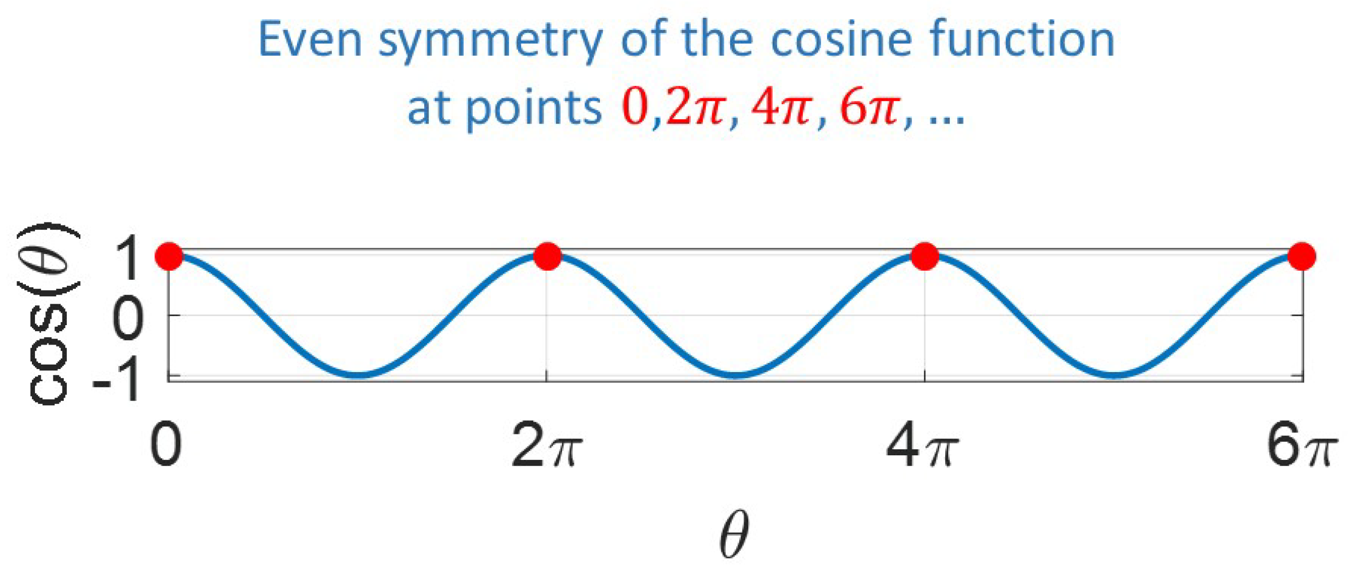
3.7. Scheme 4—Odd-Symmetry 2D FFT

Finally, in this scheme the original list of coefficients is duplicated and mirrored in each direction exactly as in Section 3.6. However, this scheme also takes advantage of the even symmetry of the cosine function at 2 k π ( k N , see Figure 6). Similar to the 1D odd-symmetry approach, the duplicated coefficients are mirrored in each direction (rows and columns), and multiplied by 1 . The final temperature is retrieved from the real component of the 2D FFT, which considers the sine components and the cosine components (that become 0 due to the cosine symmetry). The mathematical proof of the scheme is presented in Appendix D.
Algorithm 4 presents the method used to retrieve the temperature of Equation (A16) at any given time t using a 2D FFT. Line 1 initializes the extended matrix of Fourier coefficients with M , N trailing zeros. Similar to the 1D odd symmetry method, Lines 3-8 add the reversed sequences of Fourier coefficients (with negative sign) in each direction (see Figure 5). Line 9 computes the 2D FFT of the extended Fourier matrix. Line 11 extracts the real part of the FFT solution and removes the mirrored part. Finally, Line 12 applies the initial and boundary conditions. The complexity of the presented algorithm is O ( M N log ( M N ) ) .
Algorithm 4 Retrieve temperature using 2D FFTs by applying odd sine symmetry and even cosine symmetry to the original coefficients
Require: Θ R ( M 2 ) × ( N 2 ) , u R
Ensure: U R M × N
1:
Θ O D D _ S Y M zeros ( 2 M , 2 N )
2:
Θ O D D _ S Y M [ 1 : M 1 , 1 : M 1 ] Θ
3:
for m = M + 1 , m < 2 M 1 , m m + 1 do
4:
Θ O D D _ S Y M [ m , : ] Θ O D D _ S Y M [ 2 M m 1 ]
5:
end for
6:
for n = N + 1 , n < 2 N 1 , n n + 1 do
7:
Θ O D D _ S Y M [ n , : ] Θ O D D _ S Y M [ 2 N n 1 ]
8:
end for
9:
M a t fft 2 d ( Θ O D D _ S Y M )
10:
U zeros ( M , N )
11:
U real ( M a t [ 0 : M 1 , 0 : N 1 ] )
12:
U U + u
13:
returnU.

3.8. Complexity Analysis

This section presents a complexity analysis of the presented algorithms. Table 1, presents the computational complexity of Algorithm 2, line by line. The number of operations in a 1D FFT is of N + N log N [2,34]. As M and N grow large, the dominant term for the total number of computer operations is 2 M N ( log ( 2 M ) + log ( 2 N ) ) . As a consequence, the resulting complexity is O ( M N ( log M + log N ) ) or equivalently, O ( M N log ( M N ) ) .
Algorithms 1, 3 and 4, present the same structure as Algorithm 2 does. Therefore, similar complexity analysis apply for Algorithms 1, 2, 3 and 4, resulting in the same complexity order O ( M N log ( M N ) ) .

4. Results

This section presents the simulation and performance results of the implemented DST and FFT schemes using different state-of-the-art FFT libraries, for the solution of the laser heating problem on thin metal plates. All the simulations are executed with the parameters presented in Table 2 and the laser trajectory presented in Figure 2a. Section 4.1 presents the numerical validation of the presented schemes with respect to the brute-force algorithms [22,23,24,25]. Finally, Section 4.2 discusses the computational performance of the implemented schemes using available FFT libraries.

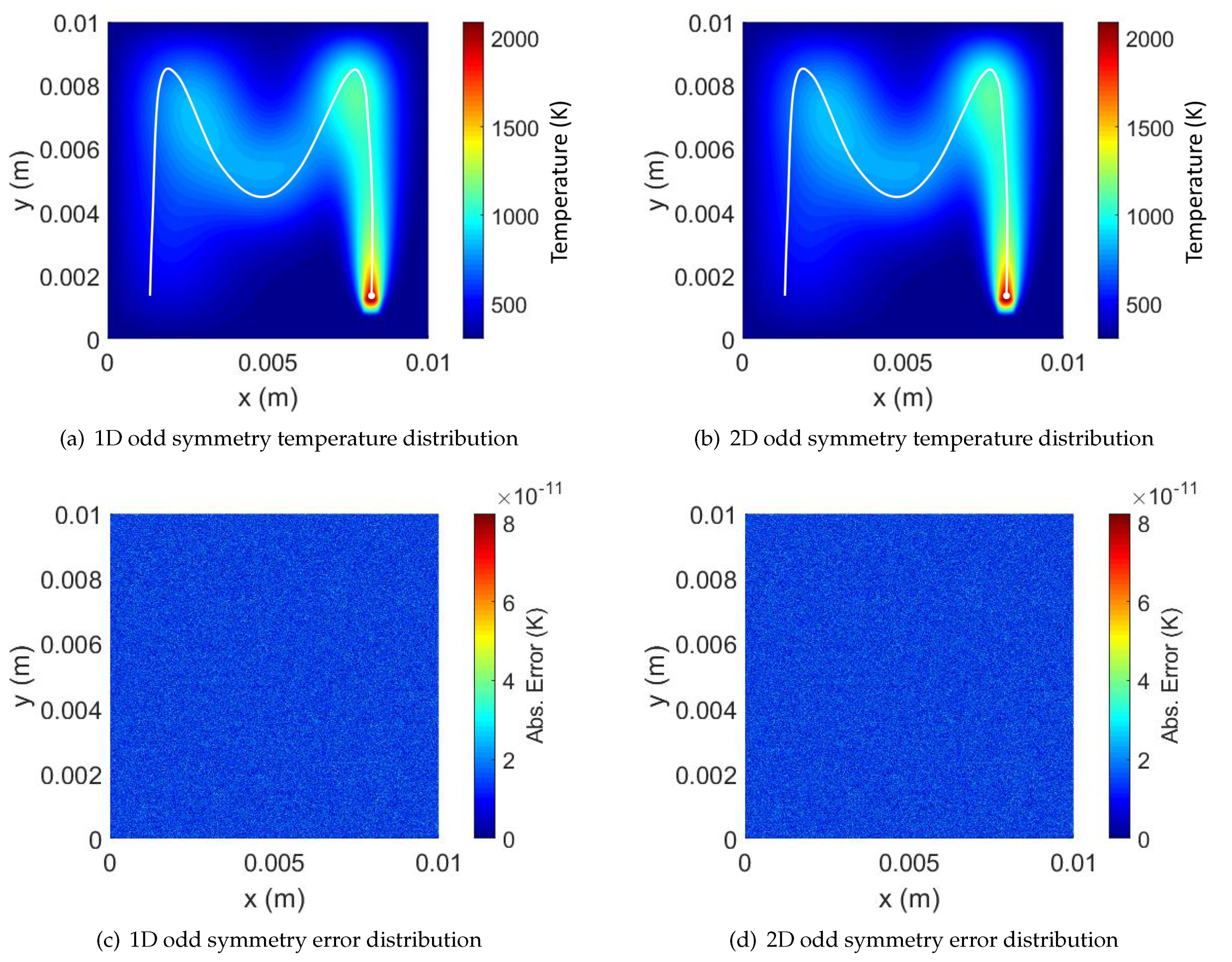
4.1. Numerical Validation

Section 3 validates the mathematical correctness of the presented schemes. However, a numerical validation is presented in this section with numerical and graphical results for a 0.01 × 0.01 × 0.001 rectangular plate. Laser and material parameters are presented in Table 2 while the laser trajectory used for the tests is the same presented in Figure 2a. As a groundtruth, we choose the method presented in References [23,24,25]. This method already solves the problem presented in Equation (1) using a brute-force approach, which requires O ( M 2 N 2 ) operations (as already discussed in Section 3.3. Figure 7 plots the temperature distribution results obtained with this brute-force method.
Figure 8a plots the temperature distribution at the end of the laser trajectory, computed with the DST algorithm for a 1024 × 1024 plate discretization. Figure 8b plots the same result computed with the zero padding FFT algorithm. The absolute error for the DST and the zero paddding FFT result (w.r.t. the brute-force approach) is presented in Figure 8c,d, respectively. The measured absolute error is below 10 10 (K) in both cases. It is worth pointing out that this error is evenly distributed through the 2D plate, which means that such error is not sensitive to the laser path or any other geometric features (such as the domain boundaries).
Similarly, Figure 9a,b plot the temperature distributions at the end of the laser trajectory for the 1D symmetric FFT and the 2D symmetric FFT algorithms, respectively. Figure 9c,d plot the absolute error for the 1D symmetric and 2D symmetric FFTs, respectively. Again, the error is below 10 10 , evenly distributed through the 2D plate.

4.2. Computational Performance

This section evaluates the performance of the proposed methods under CPU and GPU hardware architectures by making use of highly optimized FFT libraries. The Python programming language includes in its scientific package ecosystem high level wrappers to C/C++ libraries. For this reason, Python has been selected for the rapid prototyping of the proposed schemes in this work.
The FFT algorithm is used in a wide range of performance demanding applications. Therefore, the optimization degree of its implementation is highly relevant. On the one hand, to target the CPU, the FTTPACK, MKL and FFTW libraries have been selected. On the other hand, to target the GPU, the cuFFT library from the NVIDIA CUDA Toolkit has been used. All these libraries make use of multi-core parallelization, vectorization instructions, efficient memory usage, and apply specific FFT algorithms to exploit the underlying hardware to the highest degree. It is worth noticing that the FFTPACK library is the only one (between the aforementioned ones) that provides an implementation of the DST.
Table 3 summarizes the selected libraries along the Python wrapper packages and the targeted hardware device during the performance tests.
Two test platforms have been used for the performance measurements: (i) a desktop PC using Windows 10 with an Intel Core i5-6500 (CPU), 16 GB RAM and NVIDIA GeForce GTX 960 (GPU) and (ii) a desktop PC using Manjaro (GNU/Linux) with an Intel Core i7-4700K (CPU), 16GB RAM and NVIDIA GeForce RTX 2060 (GPU). To measure the execution times of each proposed method, each test has been computed 5 times and the minimum time has been registered.
This section is divided into four subsections. Section 4.2.1 presents the computation times using the CPU, while Section 4.2.2 presents the computational times using GPU hardware. Then, Section 4.2.3 compares the performance difference between both devices. Finally, Section 4.2.4 presents the achieved speed-up against the state of the art brute-force solution [22,23,24,25].

4.2.1. CPU Performance Measurements

Figure 10 shows the computation time of the proposed schemes using the FFTPACK, MKL and FFTW libraries, respectively. These are all implemented to be executed in general CPU hardware.
Figure 10a,b show all the proposed schemes implemented with the FFTPACK library. The FFTPACK is the only library (between the used ones in this manuscripts) that has an implementation of the DST algorithm. This DST implementation is efficient for plate discretization sizes of 512 × 512 and 1024 × 1024 . However, its performance is not as consistent as the FFT based methods. Overall, the performance of the FFT-based methods with different input size are more stable, being the 1D odd symmetric FFT scheme the best approach using the FFTPACK library.
Figure 10c,d show the execution times of the temperature evaluation making use of the MKL library. In this case, from the FFT-based methods, both the 1D and 2D odd symmetric schemes are the most efficient.
Figure 10e,f show the computation times using the FFTW library. Although, quite close to the results obtained with the MKL library, the FFTW results are the best when using the CPU device. In this case, also both the 1D and 2D odd symmetric schemes are the most efficient.
The optimization degree achieved for the FFT algorithms with the MKL and FFTW libraries is higher. These libraries make better use of the underlying hardware, obtaining faster results than the FFTPACK library for the FFT-based methods. Results obtained with the FFTW library are slightly better (faster) than the MKL ones. However, this can be due to the usage of wrappers, as the pyfftw (FFTW) wrapper offers more control over the implementation. Nonetheless, the obtained results greatly surpass the state of art, both FFTW and MKL have shown execution times under 1s for plate sizes up to 4096 × 4096 .

4.2.2. GPU Performance Measurements

Figure 11 shows the computation time for the three proposed FFT schemes using different GPU hardware: (i) GeForce GTX 960 and (ii) GeForce RTX 2060. The implementation is based on the cuFFT (CUDA toolkit) library and makes use of the PyCUDA and scikit-cuda python packages.
While the zero padding and the 1D odd symmetric implementations produce similar results (in terms of computation time), the 2D odd symmetric scheme is by far the most performant. As the Fourier coefficients can be computed in the GPU before performing the temperature computation, the input for the FFT is already in GPU memory. It is worth to point out that the transfer of these coefficients from host memory (CPU) to device memory (GPU) is not measured.

4.2.3. Comparison of CPU and GPU Performance

Figure 12a shows an overview of the computation times for the proposed DST (FFTPACK only) and FFT (FFTPACK, MKL, FFTW and cuFFT) methods. The FFTPACK (red) is the slowest and cuFFT (yellow) is the fastest. Execution times for both the MKL (blue) and FFTW (green) libraries are similar, obtaining slightly faster results with FFTW. Overall, the GPU hardware acceleration (with cuFFT) provides a considerable speed-up, making it a good alternative to consider for simulations on plates with large discretization sizes.
Figure 12b compares the execution times of the two test platforms considering both CPU and GPU devices for the most performant FFT method: the 2D odd symmetric algorithm. This comparison shows that the GPU hardware effectively accelerates the computation time, between the fastest CPU (i7-4700K) and the slowest GPU (GTX 960), obtaining up to a 2 × speed-up for plate sizes larger than 1024 × 1024 . The performance difference increases as the input plate increases in size. Using more recent GPU hardware (RTX 2060) results show a bigger difference in the achievable compute time speed-up.

4.2.4. Comparison against State of the Art

Figure 13 compares the proposed FFT method with the state of the art (SoA) GPU brute-force solution [25]. The presented FFT method is much faster for plate sizes larger than 128 × 128 , showing a big difference in computing times with a plate size of 1024 × 1024 , where the FFT approach obtains a 124 × speed-up (2.255 s against 0.018 s). Figure 13 demonstrates the potential of the presented FFT method to perform the temperature evaluation for high resolution plate sizes ( 1024 × 1024 and beyond). Furthermore, the current brute-force solution [25] has a limit size of 1024 × 1024 due to GPU shared memory usage, while the proposed FFT approach can compute the temperature for plates of sizes up to 4096 × 4096 under the same GPU hardware, without resorting to out-of-core GPU memory management. For small plate sizes (smaller than 128 × 128 ), the brute-force approach is faster due to the FFT method requiring extra processing of input coefficients and dispatching of kernels (scheduling time), adding a small computation overhead.

4.3. Interactive Simulator Prototype

This section presents the integration of the presented FFT-based schemes into a 3D interactive simulator for CNC (Computer Numeric Control) laser machining. The prototype integrates a physical module for the temperature computation and a geometry module that computes the plate cutting through time [23]. The physical module implements the GPU-based FFT algorithms presented in this manuscript for the temperature computation at interactive rates while the geometry module performs boolean operations as discussed in References [38,39].
The current prototype provides interactive simulation of the laser heating/cutting process, visualized as a continuous animation. Interactively, the user can inspect the plate and its temperature at any specific timestep. Furthermore, the fast computation speed enables the possibility to run different simulations with different parameters in an interactive manner. Figure 14 shows the virtual simulator for the test case discussed in this manuscript.
The development of interactive virtual worlds connected with physical objects (e.g., digital twins), has become a key technology for fast assessment of manufacturing processes [1]. In this context, an interactive CNC machine (as the integrated prototype) provides several tools to the engineer for the design of efficient CNC programs (plate, laser parameters and trajectory), reducing the requirement of real-world tests and consequently, reducing costs in terms of energy consumption, material waste, machining times, and so forth.
The performance of the simulation is very important in the decision making process and particularly, in the optimization of a given CNC program. Given a fixed time to design the CNC program, it is important to test and tune the different program parameters (such as laser parameters and trajectory). The current approach shows a significant decrease in the simulation computing time. This saving allows user-assisted and/or automated optimization programs to evaluate the different scenarios at a reasonable computational cost. The impact of such optimization on the quality of the workpiece will depend on the actual decisions and strategies applied by the engineers, supported by the simulation results.
Although not being part of the present investigation, it is worth noticing that the temperature maps on the plate help to predict and control deformations caused by thermal residual stresses.

5. Conclusions and Future Work

This manuscript presents four different schemes for the solution of the laser heating problem on thin metal plates using the DST and the FFT. The presented methods reduce the computational complexity of the problem from O ( M 2 N 2 ) to O ( M N log ( M N ) ) (with M × N being the discretization size of the metal plate). It is worth noting that forced convection and radiative heat transfer are not present in the solution considered in this manuscript. The inclusion of those effects in the simulation implies a significant change in the structure of the mathematical model, which is out of the scope of this research. Overcoming of such a limitation is left as future work.
These schemes are implemented in both CPU and GPU architectures using available optimized FFT libraries. Mathematical and numerical proofs of the correctness of the schemes are presented and the numerical error is measured below 10 10 K (and independent of the laser trajectory).
The performance evaluation shows that the minimum achievable computation time varies in function of the used library, specially for big input sizes. Furthermore, the obtained results improve the state of the art [25] in both CPU and GPU platforms for all the proposed schemes. Specifically, using GPU hardware, the computation times for the temperature evaluation are reduced from 1 s to 0.01 s ( 100 × faster), measured in an NVIDIA GeForce GTX 960 (GPU).
With more modern GPU hardware (GeForce RTX2060) even faster results can be acquired which shows the potential of the proposed algorithms towards real-time laser heating/cutting simulations and flexible manufacturing scenarios that require fast tool-planning capability and laser parameter optimization to easily adapt to customer order changes.
Future work includes (1) the inclusion of thermal/stress models for structural analysis of the plate after the generated high temperature gradients, (2) analysis of non-rectangular plate geometries, and (3) consideration of non-linear interactions such as temperature-dependent thermal properties, forced convection, radiation heat transfer and phase changes.

Author Contributions

D.M.-P., A.A. and A.M. conceived, designed and implemented the algorithms and performed the simulations. O.R.-S. and J.P. supervised the Computational Geometry, Heat Transfer and Spectral Methods research. J.L.-P. supervised the Parallel Computing, Data Structures and High Performance Programming aspects of this research. All the authors contributed to the writing of this manuscript. All authors have read and agreed to the published version of the manuscript.

Funding

This research received no external funding.

Conflicts of Interest

The authors declare no conflict of interest.

Abbreviations

The following abbreviations are used in this manuscript:
PDEPartial Differential Equation
DSTDiscrete Sine Transform
DFTDiscrete Fourier Transform
FFTFast Fourier Transform
a , b , Δ z Width, height and thickness of the thin plate (m3).
T f Total simulation time (s).
x , t Spatial x = ( x , y ) [ 0 , a ] × [ 0 , b ] and temporal 0 t T f coordinates.
u = u ( x , t ) Temperature field u : [ 0 , a ] × [ 0 , b ] × [ 0 , T f ] R on the metal plate (K).
ρ Plate density (kg/m3).
c p Plate specific heat (J/kg K).
κ Plate thermal conductivity (W/m K).
RPlate reflectivity ( 0 R < 1 ).
q = q ( u ) Temperature-dependent heat convection field q : R R (W/m2).
hNatural convection coefficient at the plate surface (W/(m2 K))
u Ambient temperature (K).
x 0 = x 0 ( t ) Laser spot location at a given time x 0 ( t ) = ( x 0 ( t ) , y 0 ( t ) ) .
f = f ( x , t ) Power Density Field f : [ 0 , a ] × [ 0 , b ] × [ 0 , T f ] R for the laser beam (W/m2).
PLaser power (W).
rLaser spot radius (m).
M × N 2D plate discretization size ( M , N N ).
θ m n ( t ) m t h , n t h Fourier coefficient ( m , n = 0 , 1 , ) for the temperature solution u at time t.
α m , β n Coefficients α m = ( m + 1 ) π / a and β n = ( n + 1 ) π / b for the Fourier basis in the X- and Y-axis, respectively.
γ m , δ n γ m = m π / M and δ n = n π / N are the discrete equivalent of α m ( m = 0 , 1 , , M 1 ) and β n ( n = 0 , 1 , , N 1 ), respectively.
ω m n m t h , n t h eigenvalue of the heat (Laplace) operator defined on the rectangular plate.
C i ( t ) Piecewise linear discretization of the laser trajectory x 0 ( t ) .

Appendix A. Scheme 1—Discrete Sine Transform (DST)

Let { x 0 , x 1 , , x M } and { y 0 , y 1 , , y N } be uniform discretizations of the intervals [ 0 , a ] and [ 0 , b ] , respectively. It is worth noting that for such a uniform sampling, the equalities x k / a = i / M and y l / b = l / N hold. Therefore, after truncating the number of Fourier coefficients to ( M 1 ) × ( N 1 ) , Equation (3) is approximated as:
u k l ( t ) = u + m = 0 M 2 n = 0 N 2 θ m n sin ( γ m + 1 k ) sin ( δ n + 1 l ) , k = 0 , 1 , M 1 , l = 0 , 1 , , N 1
with u k l ( t ) = u ( x k , y l , t ) the temperature at the discrete points of the plate and γ m = m π / M , δ n = n π / N the discrete versions of α m and β n , respectively. This equation is equivalent to a 2D DST of the temperatures on the discrete plate (as per Equation (8)).

Appendix B. Scheme 2—FFT Padded with Zeros

Consider { x 0 , x 1 , , x M } be a uniform discretization of the interval [ 0 , a ] . For M Fourier coefficients the following equation holds:
m = 0 M 2 θ m n sin ( γ ( m + 1 ) k ) = I m = 0 M 2 θ m n i sin 2 γ ( m + 1 ) k 2 = I m = 0 M 2 θ m n e i 2 π 2 M k ( m + 1 ) n = 0 , 1 , N 1
where I [ · ] corresponds to the complex component of the series and γ m = m π / M . This corresponds to a 1D DFT (Equation (7)) with M trailing zeros.
After applying the same procedure to the sequence { y 0 , y 1 , , y N } , Equation (3) becomes:
u k l ( t ) = u + I n = 0 N 2 I m = 0 M 2 θ m n e i 2 π 2 M k ( m + 1 ) e i 2 π 2 N l ( n + 1 ) , k = 0 , 1 , M 1 , l = 0 , 1 , , N 1
The previous equation is equivalent to 2 nested 1D DFTs (Equation (7)) after adding 1 zero at the beginning of the Fourier sequence and M, N zeros (x and y components, respectively) at the end of the sequence.

Appendix C. Scheme 3—Odd-Symmetry 1D FFT

Consider { x 0 , x 1 , , x M } be a uniform discretization of the interval [ 0 , a ] . Since sin ( x ) = sin ( x ) and sin ( x ) = sin ( x + 2 k π ) (with k N + ) the following equation holds:
m = 0 M 2 θ m n sin ( m + 1 ) k π M = m = 0 M 2 θ m n sin ( m + 1 ) k π M = m = 0 M 2 θ m n sin ( m + 1 ) k π M + 2 k π = m = 0 M 2 θ m n sin ( 2 M m 1 ) k π M , n = 0 , 1 , N
The previous series can be expressed in reverse form by setting m M m 2 :
m = 0 M 2 θ m n sin ( m + 1 ) k π M = m = 0 M 2 θ ( M m 2 ) n sin ( M + m + 1 ) k π M
Afterwards, consider the sequence shift m = M + 1 , M + 2 , , 2 M 1 . Equation (A5) becomes:
m = 0 M 2 θ m n sin ( m + 1 ) k π M = m = M + 1 2 M 1 θ ( 2 M m 1 ) n sin m k π M
which is the second half of a sine transform with negative coefficients in reverse order. Therefore, the series can be split in two as follows:
m = 0 M 2 θ m n sin ( m + 1 ) k π M = 1 2 m = 0 M 2 θ m n sin ( m + 1 ) k π M + 1 2 m = M + 1 2 M 1 θ ( 2 M m 1 ) n sin m k π M
On the other hand, from Equation (7):
ϕ m sin m k π M = I ϕ m i sin 2 m k π 2 M = I ϕ m e i 2 π 2 M k m
where I [ · ] corresponds to the complex component of the Fourier term.
Putting together Equations (A7) and (A8), Equation (3) becomes:
u k l ( t ) = u + 1 4 I n = 0 N 2 I m = 0 M 2 θ m n e i 2 π 2 M k ( m + 1 ) e i 2 π 2 N l ( n + 1 ) 1 4 I n = 0 N 2 I m = M + 1 2 M 1 θ ( 2 M m 1 ) n e i 2 π 2 M k m e i 2 π 2 N l ( n + 1 ) 1 4 I n = N + 1 2 N 1 I m = 0 M 2 θ m ( 2 N n 1 ) e i 2 π 2 M k ( m + 1 ) e i 2 π 2 N l n + 1 4 I n = N + 1 2 N 1 I m = M + 1 2 M 1 θ ( 2 M m 1 ) ( 2 N n 1 ) e i 2 π 2 M k m e i 2 π 2 N l n k = 0 , 1 , M 1 , l = 0 , 1 , , N 1
The previous equation is equivalent to 2 nested 1D DFTs (Equation (7)) after padding the M 2 , N 2 coefficients in reverse order (and negative) at the end of the original Fourier coefficients in each direction (x and y), respectively. The final result is retrieved by taking the complex part (i.e., the sine component) of each 1D DFT.

Appendix D. Scheme 4—Odd-Symmetry 2D FFT

In this scheme, consider the real part D k l (instead of the complex one) of Equation (A9) as follows:
D k l = 1 4 R e n = 0 N 2 R e m = 0 M 2 θ m n e i 2 π 2 M k ( m + 1 ) e i 2 π 2 N l ( n + 1 ) 1 4 R e n = 0 N 2 R e m = M + 1 2 M 1 θ ( 2 M m 1 ) n e i 2 π 2 M k m e i 2 π 2 N l ( n + 1 ) 1 4 R e n = N + 1 2 N 1 R e m = 0 M 2 θ m ( 2 N n 1 ) e i 2 π 2 M k ( m + 1 ) e i 2 π 2 N l n + 1 4 R e n = N + 1 2 N 1 R e m = M + 1 2 M 1 θ ( 2 M m 1 ) ( 2 N n 1 ) e i 2 π 2 M k m e i 2 π 2 N l n k = 0 , 1 , M 1 , l = 0 , 1 , , N 1
which in fact consists of the cosine parts of the Fourier series:
D k l = 1 4 n = 0 N 2 m = 0 M 2 θ m n cos 2 π k ( m + 1 ) 2 M cos 2 π l ( n + 1 ) 2 N 1 4 n = 0 N 2 m = M + 1 2 M 1 θ ( 2 M m 1 ) n cos 2 π k m 2 M cos 2 π l ( n + 1 ) 2 N 1 4 n = N + 1 2 N 1 m = 0 M 2 θ m ( 2 N n 1 ) cos 2 π k ( m + 1 ) 2 M cos 2 π l n 2 N + 1 4 n = N + 1 2 N 1 m = M + 1 2 M 1 θ ( 2 M m 1 ) ( 2 N n 1 ) cos 2 π k m 2 M cos 2 π l n 2 N k = 0 , 1 , M 1 , l = 0 , 1 , , N 1
Consider the second term of the previous expansion, and the change of the series variable m 2 M m 1 . Since cos ( x ) = cos ( x ) and cos ( x ) = cos ( x + 2 π k ) (with k N + ), then the following equation holds:
1 4 n = 0 N 2 m = M + 1 2 M 1 θ ( 2 M m 1 ) n cos 2 π k m 2 M cos 2 π l ( n + 1 ) 2 N = 1 4 n = 0 N 2 m = 0 M 2 θ m n cos 2 π k ( 2 M 1 m ) 2 M cos 2 π l ( n + 1 ) 2 N = 1 4 n = 0 N 2 m = 0 M 2 θ m n cos 2 π k ( m + 1 ) 2 M cos 2 π l ( n + 1 ) 2 N
Applying the same procedure to the fourth term in Equation (A11), we obtain:
1 4 n = N + 1 2 N 1 m = M + 1 2 M 1 θ ( 2 M m 1 ) ( 2 N n 1 ) cos 2 π k m 2 M cos 2 π l n 2 N = 1 4 n = N + 1 2 N 1 m = 0 M 2 θ m ( 2 N n 1 ) cos 2 π k ( 2 M 1 m ) 2 M cos 2 π l n 2 N = 1 4 n = N + 1 2 N 1 m = 0 M 2 θ m ( 2 N n 1 ) cos 2 π k ( m + 1 ) 2 M cos 2 π l n 2 N
Substituting Equations (A12) and (A13) into Equation (A11):
D k l = 1 4 n = 0 N 2 m = 0 M 2 θ m n cos 2 π k ( m + 1 ) 2 M cos 2 π l ( n + 1 ) 2 N 1 4 n = 0 N 2 m = 0 M 2 θ m n cos 2 π k ( m + 1 ) 2 M cos 2 π l ( n + 1 ) 2 N 1 4 n = N + 1 2 N 1 m = 0 M 2 θ m ( 2 N n 1 ) cos 2 π k ( m + 1 ) 2 M cos 2 π l n 2 N + 1 4 n = N + 1 2 N 1 m = 0 M 2 θ m ( 2 N n 1 ) cos 2 π k ( m + 1 ) 2 M cos 2 π l n 2 N k = 0 , 1 , M 1 , l = 0 , 1 , , N 1
in which the first and second terms cancel out, as well as terms three and four, respectively. Therefore:
k , l D k l = 0
Finally, we add D k l to Equation (A9):
u k l ( t ) = u k l ( t ) + D k l = u + 1 4 R e n = 0 N 2 m = 0 M 2 θ m n e i 2 π 2 M k ( m + 1 ) e i 2 π 2 N l ( n + 1 ) 1 4 R e n = 0 N 2 m = M + 1 2 M 1 θ ( 2 M m 1 ) n e i 2 π 2 M k m e i 2 π 2 N l ( n + 1 ) 1 4 R e n = N + 1 2 N 1 m = 0 M 2 θ m ( 2 N n 1 ) e i 2 π 2 M k ( m + 1 ) e i 2 π 2 N l n + 1 4 R e n = N + 1 2 N 1 m = M + 1 2 M 1 θ ( 2 M m 1 ) ( 2 N n 1 ) e i 2 π 2 M k m e i 2 π 2 N l n k = 0 , 1 , M 1 , l = 0 , 1 , , N 1
The above equation is true since R e ( x y ) = R e ( x ) R e ( y ) + I ( x ) I ( y ) (i.e., the real part of the product of two complex numbers is the sum of their real parts and their imaginary parts). Equation (A16) is equivalent to a 2D DFT (Equation (7)) after padding the M 2 , N 2 coefficients in reverse order (and negative) at the end of the original Fourier coefficients in each direction (x and y), respectively. The final result is retrieved by taking the real part of the result.

References

  1. Posada, J.; Toro, C.; Barandiaran, I.; Oyarzun, D.; Stricker, D.; de Amicis, R.; Pinto, E.B.; Eisert, P.; Döllner, J.; Vallarino, I. Visual Computing as a Key Enabling Technology for Industrie 4.0 and Industrial Internet. IEEE Comput. Graphics Appl. 2015, 35, 26–40. [Google Scholar] [CrossRef]
  2. Cooley, J.W.; Tukey, J.W. An algorithm for the machine calculation of complex Fourier series. Math. Comput. 1965, 19, 297–301. [Google Scholar] [CrossRef]
  3. Mejia-Parra, D.; Arbelaiz, A.; Moreno, A.; Posada, J.; Ruiz-Salguero, O. Fast Spectral Formulations of Thin Plate Laser Heating with GPU Implementations. In Proceedings of the 2nd International Conference on Mathematics and Computers in Science and Engineering (MACISE 2020), Madrid, Spain, 18–20 January 2020. to be Published. [Google Scholar]
  4. Yilbas, B.S.; Akhtar, S.; Keles, O. Laser cutting of triangular blanks from thick aluminum foam plate: Thermal stress analysis and morphology. Appl. Therm. Eng. 2014, 62, 28–36. [Google Scholar] [CrossRef]
  5. Akhtar, S.; Kardas, O.O.; Keles, O.; Yilbas, B.S. Laser cutting of rectangular geometry into aluminum alloy: Effect of cut sizes on thermal stress field. Opt. Lasers Eng. 2014, 61, 57–66. [Google Scholar] [CrossRef]
  6. Yilbas, B.; Akhtar, S.; Karatas, C. Laser cutting of rectangular geometry into alumina tiles. Opt. Lasers Eng. 2014, 55, 35–43. [Google Scholar] [CrossRef]
  7. Akhtar, S.S. Laser cutting of thick-section circular blanks: Thermal stress prediction and microstructural analysis. Int. J. Adv. Manuf. Technol. 2014, 71, 1345–1358. [Google Scholar] [CrossRef]
  8. Roberts, I.; Wang, C.; Esterlein, R.; Stanford, M.; Mynors, D. A three-dimensional finite element analysis of the temperature field during laser melting of metal powders in additive layer manufacturing. Int. J. Mach. Tools Manuf. 2009, 49, 916–923. [Google Scholar] [CrossRef]
  9. Shi, B.; Attia, H. Integrated Process of Laser-Assisted Machining and Laser Surface Heat Treatment. J. Manuf. Sci. Eng. 2013, 135, 061021. [Google Scholar] [CrossRef]
  10. Akarapu, R.; Li, B.Q.; Segall, A. A thermal stress and failure model for laser cutting and forming operations. J. Fail. Anal. Prev. 2004, 4, 51–62. [Google Scholar] [CrossRef]
  11. Nyon, K.Y.; Nyeoh, C.Y.; Mokhtar, M.; Abdul-Rahman, R. Finite element analysis of laser inert gas cutting on Inconel 718. Int. J. Adv. Manuf. Technol. 2012, 60, 995–1007. [Google Scholar] [CrossRef]
  12. Fu, C.; Sealy, M.; Guo, Y.; Wei, X. Finite element simulation and experimental validation of pulsed laser cutting of nitinol. J. Manuf. Process. 2015, 19, 81–86. [Google Scholar] [CrossRef]
  13. Modest, M.F. Three-dimensional, transient model for laser machining of ablating/decomposing materials. Int. J. Heat Mass Transf. 1996, 39, 221–234. [Google Scholar] [CrossRef]
  14. Han, G.-c.; Nas, S.-j. A Study on Torch Path Planning in Laser Cutting Processes Part 1: Calculation of Heat Flow in Contour Laser Beam Cutting. J. Manuf. Process. 1999, 1, 54–61, Special Issue of the Journal of Manufacturing Systems. [Google Scholar] [CrossRef]
  15. Xu, W.; Fang, J.; Wang, X.; Wang, T.; Liu, F.; Zhao, Z. A numerical simulation of temperature field in plasma-arc forming of sheet metal. J. Mater. Process. Technol. 2005, 164–165, 1644–1649, AMPT/AMME05 Part 2. [Google Scholar] [CrossRef]
  16. Kim, M.J. Transient evaporative laser-cutting with boundary element method. Appl. Math. Model. 2000, 25, 25–39. [Google Scholar] [CrossRef]
  17. Kim, M.J. Transient evaporative laser cutting with moving laser by boundary element method. Appl. Math. Model. 2004, 28, 891–910. [Google Scholar] [CrossRef] [Green Version]
  18. Kheloufi, K.; Hachemi Amara, E.; Benzaoui, A. Numerical Simulation of Transient Three-Dimensional Temperature and Kerf Formation in Laser Fusion Cutting. J. Heat Transf. 2015, 137, 112101. [Google Scholar] [CrossRef]
  19. Yuan, P.; Gu, D. Molten pool behaviour and its physical mechanism during selective laser melting of TiC/AlSi10Mg nanocomposites: Simulation and experiments. J. Phys. D Appl. Phys. 2015, 48, 035303. [Google Scholar] [CrossRef]
  20. Zimmer, K. Analytical solution of the laser-induced temperature distribution across internal material interfaces. Int. J. Heat Mass Transf. 2009, 52, 497–503. [Google Scholar] [CrossRef]
  21. Modest, M.F.; Abakians, H. Evaporative Cutting of a Semi-infinite Body With a Moving CW Laser. J. Heat Transf. 1986, 108, 602–607. [Google Scholar] [CrossRef]
  22. Jiang, H.J.; Dai, H.L. Effect of laser processing on three dimensional thermodynamic analysis for HSLA rectangular steel plates. Int. J. Heat Mass Transf. 2015, 82, 98–108. [Google Scholar] [CrossRef]
  23. Mejia, D.; Moreno, A.; Arbelaiz, A.; Posada, J.; Ruiz-Salguero, O.; Chopitea, R. Accelerated Thermal Simulation for Three-Dimensional Interactive Optimization of Computer Numeric Control Sheet Metal Laser Cutting. J. Manuf. Sci. Eng. 2017, 140, 031006. [Google Scholar] [CrossRef]
  24. Mejia-Parra, D.; Moreno, A.; Posada, J.; Ruiz-Salguero, O.; Barandiaran, I.; Poza, J.C.; Chopitea, R. Frequency-domain analytic method for efficient thermal simulation under curved trajectories laser heating. Math. Comput. Simul. 2019, 166, 177–192. [Google Scholar] [CrossRef]
  25. Mejia-Parra, D.; Montoya-Zapata, D.; Arbelaiz, A.; Moreno, A.; Posada, J.; Ruiz-Salguero, O. Fast Analytic Simulation for Multi-Laser Heating of Sheet Metal in GPU. Materials 2018, 11, 2078. [Google Scholar] [CrossRef] [PubMed] [Green Version]
  26. Ju, Y.; Farris, T.N. FFT Thermoelastic Solutions for Moving Heat Sources. J. Tribol. 1997, 119, 156–162. [Google Scholar] [CrossRef]
  27. Dillenseger, J.L.; Esneault, S. Fast FFT-based bioheat transfer equation computation. Comput. Biol. Med. 2010, 40, 119–123. [Google Scholar] [CrossRef] [Green Version]
  28. Berbenni, S.; Taupin, V.; Djaka, K.S.; Fressengeas, C. A numerical spectral approach for solving elasto-static field dislocation and g-disclination mechanics. Int. J. Solids Struct. 2014, 51, 4157–4175. [Google Scholar] [CrossRef]
  29. Djaka, K.S.; Villani, A.; Taupin, V.; Capolungo, L.; Berbenni, S. Field Dislocation Mechanics for heterogeneous elastic materials: A numerical spectral approach. Comput. Methods Appl. Mech. Eng. 2017, 315, 921–942. [Google Scholar] [CrossRef] [Green Version]
  30. Ma, R.; Truster, T.J. FFT-based homogenization of hypoelastic plasticity at finite strains. Comput. Methods Appl. Mech. Eng. 2019, 349, 499–521. [Google Scholar] [CrossRef]
  31. Paramatmuni, C.; Kanjarla, A.K. A crystal plasticity FFT based study of deformation twinning, anisotropy and micromechanics in HCP materials: Application to AZ31 alloy. Int. J. Plast. 2019, 113, 269–290. [Google Scholar] [CrossRef]
  32. Starn, J. A Simple Fluid Solver Based on the FFT. J. Graphics Tools 2001, 6, 43–52. [Google Scholar] [CrossRef]
  33. Taboada, J.M.; Landesa, L.; Obelleiro, F.; Rodriguez, J.L.; Bertolo, J.M.; Araujo, M.G.; Mouri no, J.C.; Gomez, A. High Scalability FMM-FFT Electromagnetic Solver for Supercomputer Systems. IEEE Antennas Propag. Mag. 2009, 51, 20–28. [Google Scholar] [CrossRef]
  34. Manolakis, D.; Ingle, V. Chapter 8—Computation of the Discrete Fourier Transform. In Applied Digital Signal Processing: Theory and Practice; Manolakis, D., Ingle, V., Eds.; Cambridge University Press: New York, NY, USA, 2011; pp. 434–484. [Google Scholar]
  35. Raaf, O.; Adane, A.E.H. Pattern recognition filtering and bidimensional FFT-based detection of storms in meteorological radar images. Digit. Signal Process. 2012, 22, 734–743. [Google Scholar] [CrossRef]
  36. Britanak, V.; Yip, P.C.; Rao, K. CHAPTER 1—Discrete Cosine and Sine Transforms. In Discrete Cosine and Sine Transforms; Britanak, V., Yip, P.C., Rao, K., Eds.; Academic Press: Oxford, UK, 2007; pp. 1–15. [Google Scholar] [CrossRef]
  37. Britanak, V.; Yip, P.C.; Rao, K. CHAPTER 4—Fast DCT/DST Algorithms. In Discrete Cosine and Sine Transforms; Britanak, V., Yip, P.C., Rao, K., Eds.; Academic Press: Oxford, UK, 2007; pp. 73–140. [Google Scholar] [CrossRef]
  38. Moreno, A.; Segura, Á.; Arregui, H.; Posada, J.; Ruíz de Infante, Á.; Canto, N. Using 2D Contours to Model Metal Sheets in Industrial Machining Processes. In Future Vision and Trends on Shapes, Geometry and Algebra; De Amicis, R., Conti, G., Eds.; Springer: London, UK, 2014; pp. 135–149. [Google Scholar]
  39. Velez, G.; Moreno, A.; Infante, A.R.D.; Chopitea, R. Real-time part detection in a virtually machined sheet metal defined as a set of disjoint regions. Int. J. Comput. Integr. Manuf. 2016, 29, 1089–1104. [Google Scholar] [CrossRef]
Figure 1. Scheme for the laser heating problem on thin metal plates.
Applsci 10 03281 g001
Figure 2. Continuous laser trajectory (from point A to B) and piecewise linear discretization of the trajectory on a rectangular plate. (a) Continuous laser trajectory; (b) (Coarse) Piecewise linear discretization of the trajectory.
Applsci 10 03281 g002
Figure 3. Matrix structure for the zero padding FFT. The blue block contains the original Fourier coefficients θ m n . The remainder of the matrix is filled with zeros.
Applsci 10 03281 g003
Figure 4. Odd symmetry of the sine function at k π ( k = 0 , 1 , 2 , ).
Applsci 10 03281 g004
Figure 5. Matrix structure for the odd symmetry FFT (1D and 2D). The blue block contains the original coefficients and the remaining blocks contain their odd-symmetry counterpart. All blocks are separated by rows and columns of zeros.
Applsci 10 03281 g005
Figure 6. Even symmetry of the cosine function at 2 k π ( k = 0 , 1 , 2 , ).
Applsci 10 03281 g006
Figure 7. Temperature solution for the laser trajectory presented in Figure 2a obtained by the brute-force method [24]. No FFT or Discrete Sine Transform (DST) is used.
Applsci 10 03281 g007
Figure 8. Temperature and absolute error distributions (w.r.t. the brute-force approach [24]) on the thin plates for the DST and the zero padding FFT simulations.
Applsci 10 03281 g008
Figure 9. Temperature and absolute error distributions (w.r.t. the brute-force approach [24]) on the thin plates for the odd symmetry FFT approaches (1D and 2D).
Applsci 10 03281 g009
Figure 10. CPU computation times using the FFTPACK, MKL and FFTW libraries for the proposed schemes using different plate sizes. The odd symmetric schemes (1D and 2D) present the best performance overall.
Applsci 10 03281 g010aApplsci 10 03281 g010b
Figure 11. GPU computation times for the FFT-based methods using the cuFFT library with different plate sizes. The 2D odd symmetric scheme outperforms the remainder FFT-based ones.
Applsci 10 03281 g011
Figure 12. CPU and GPU computation time comparison using different plate resolutions. (a) Computing time for each scheme, grouped by library as per Table 3; (b) Computing time for the 2D odd symmetric FFT scheme.
Applsci 10 03281 g012
Figure 13. Appraisal of the computation times using an NVIDIA GeForce GTX960 (GPU) for the presented 2D odd symmetric FFT method vs the brute-force method presented in Reference [25]
Applsci 10 03281 g013
Figure 14. Interactive laser heating/cutting simulator. A virtual CNC machine follows the laser trajectory defined by the program and the physical module computes the temperature using the FFT.
Applsci 10 03281 g014
Table 1. Computational complexity analysis for Algorithm 2 (FFT padded with zeros). Complexity simplification rules applied are: (a) O ( k f ( n ) ) = O ( f ( n ) ) , (b) O ( f ( n ) + g ( n ) ) = O ( max ( f ( n ) , g ( n ) ) ) .
LineDescriptionNumber of OperationsDominant TermComplexity Order
1, 2Memory initialization O ( M N )
4FFT of a column 2 M + 2 M log ( 2 M ) 2 M log ( 2 M ) O ( M log M )
5Extract complex part 2 M O ( M )
3–6Loop through columns ( N 2 ) ( 4 M + 2 M log ( 2 M ) ) 2 M N log ( 2 M ) O ( M N log M )
8FFT of a row 2 N + 2 N log ( 2 N ) 2 N log ( 2 N ) O ( N log N )
9Extract complex part 2 N O ( N )
7–10Loop through rows ( M 2 ) ( 4 N + 2 N log ( 2 N ) ) 2 M N log ( 2 N ) O ( M N log M )
11, 12Memory initialization O ( M N )
13Sum of matrices M N O ( M N )
TOTAL O ( M N log M + M N log N ) = O ( M N log ( M N ) )
Table 2. Parameters for the physical simulation.
ParameterDescriptionValueUnits
aPlate width 0.01 m
bPlate height 0.01 m
Δ z Plate thickness 0.001 m
ρ Plate density8030kg/m3
c p Specific heat574J/(kg K)
κ Thermal conductivity20W/(m K)
RPlate reflectivity01
hConvection coefficient20W/(m2 K)
u Ambient temperature300K
PLaser power500W
rLaser spot radius 0.0003 m
Table 3. Selected libraries and corresponding Python packages.
LibraryPython PackageHardware
FFTPACKscipy.fftCPU
MKLnumpy.fftCPU
FFTWpyfftwCPU
cuFFTpyCUDA, scikit-cudaGPU

