
Asymptotic Analytical Solution on Lamb Waves in Functionally Graded Nano Copper Layered Wafer


School of Civil Engineering and Architecture, Xi’an University of Technology, Xi’an 710048, China
*
Author to whom correspondence should be addressed.
Appl. Sci. 2021, 11(10), 4442; https://doi.org/10.3390/app11104442
Submission received: 27 April 2021
/
Revised: 9 May 2021
/
Accepted: 11 May 2021
/
Published: 13 May 2021
(This article belongs to the Collection Nondestructive Testing (NDT))
Abstract
:In this study, the feasibility of using Lamb waves in functionally graded (FG) nano copper layered wafers in nondestructive evaluation is evaluated. The elastic parameters and mass densities of these wafers vary with thickness due to the variation in grain size. The power series technique is used to solve the governing equations with variable coefficients. To analyze multilayered structures, of which the material parameters are continuous but underivable, a modified transfer matrix method is proposed and combined with the power series method. Results show that multiple modes of Lamb waves exist in FG nano copper wafers. Moreover, the gradient property leads to a decrease in phase velocity, and the absolute value of the phase velocity variation is positively correlated with the gradient coefficient. The phase velocity variation and variation rate in Mode 2 are smaller than those in other modes. The findings indicate that Mode 4 is recommended for nondestructive evaluation. However, if the number of layers is greater than four, the dispersion curves of the Lamb waves in the multilayer structures tend to coincide with those in the equivalent uniform structures. The results of this study provide theoretical guidance for the nondestructive evaluation of FG nanomaterial layered structures.
1. Introduction
Since the introduction of functionally graded (FG) nano copper in 2011 [1], this novel material with a graded grain size distribution has attracted increasing scientific interest due to its high strength and high ductility [2,3,4]. The interest in materials with graded grain size distributions is not limited to nano copper and also includes titanium [5,6], zirconium [7], metallic glass [8], Fe–Mn austenitic steel [9], and low-carbon steel [10]. The grain refinement mechanism, microstructure characteristics, and material properties of samples of a gradient nano/microstructured surface layer on pure copper are investigated through several experiments [11]. Copper rod samples with gradient grain structures are also developed, measured in terms of microhardness, analyzed through electron backscatter diffraction, and simulated numerically [12]. With the in-depth study on FG nano copper materials [13,14] and their superiority in terms of strength and ductility, these materials will be widely utilized in engineering fields. The nondestructive evaluation of structures made of these materials is an important research topic in laboratory and engineering applications.
The guided wave technique, which is one of the most popular nondestructive evaluation methods is used to analyze Lamb, shear horizontal, Love, and Rayleigh waves. Related previous studies focused on the waves in homogenous structures [15,16]. Scientists began to investigate waves in structures made of FG materials in the 1990s. Researchers proposed various analytical methods, including directly analytical method, special function solution, the Wentzel–Kramers–Brillouin (WKB) method, the Legendre series method, and the power series method. The directly analytical method is used to solve different wave propagation problems when the material parameters vary with the same exponential function [17,18]. In this case, the governing differential equation with variable coefficients can be transformed into a differential equation with constant coefficients to obtain an analytical solution. If the governing equations can be decoupled and the material parameter variations follow specific laws, the special function method can be applied to solve wave propagation problems [19,20,21]. The WKB method is used to study the horizontal shear waves in different FG layered structures with one displacement component [22,23]. However, this approach is only applicable to wave propagation problems with large wave numbers [20]. As asymptotic methods with series form, the Legendre [24,25,26] and power series methods [27] are utilized to analyze waves in various FG structures. Especially, the Legendre series method has been applied, not only for solving wave propagation behavior of macroscopic structure [28], but also that of microstructure using the combined modified couple stress theory [29,30]. Numerical analyses of wave propagation in inhomogeneous media are also conducted. The main idea of the numerical solution is to divide the FG medium into a multilayer model. The material parameters in each layer of the model are assumed to be homogenous [31,32,33]. The transfer matrix method, which is based on the continuity of the stress and displacement in the interface, is used to solve the wave propagation problem in multilayered structures [15,34]. This numerical technique can also be applied to solve wave propagation problems in various FG layered structures [35,36]. Considering that Lamb waves have been widely used in nondestructive evaluation in engineering application, Kuznetsov analyzed and compared the similarity and discrepancy of dispersion properties of Lamb wave propagation in both functionally graded and homogeneous plates [37,38]. Considering the nondestructive evaluation of FG nano metal layered structure, we focused on different guided waves in a single layer FG nano metal wafer or a multilayered FG nano metal wafer. An early report has been published on horizontal shear (SH) waves in these structures [39].
In the present study, the Lamb waves in an FG nano copper layered structure are investigated analytically. The grain size of the FG nano copper is assumed to vary along the thickness direction, and the other material parameters are deduced using the Mori–Tanaka effective field result proposed by Wang et al. [40]. The governing differential equations for describing the Lamb waves in a simple FG nano wafer are solved using the power series method. In addition, the Lamb wave propagation problem in a multilayered FG nano metal wafer with continuous and non-differentiable material parameters is solved through a modified transfer matrix method combined with the power series technique. On the basis of the abovementioned methods, numerical examples are analyzed, and the propagation properties of the Lamb waves in an FG nano copper wafer are discussed.
2. Statement of the Problem
2.1. Governing Equations
In this study, the Lamb waves in two types of FG nano copper layered wafer are considered (Figure 1). The wave propagation direction is the positive direction of the x1 axis, and the thickness is along the x3 axis. If the grain size of the FG nano copper wafer varies with thickness and is a function of x3, then the corresponding material parameters, including the elastic parameters and mass density, are not constants, but are functions of x3. Figure 1a presents a simple FG nano copper wafer with thickness h and a monotonously changing grain size, whereas Figure 1b displays a multilayered FG nano copper wafer composed of several simple wafers with interfaces that have continuous grain sizes. The thickness of each simple wafer is h, and the total thickness is H. Therefore, the grain size is alternately increasing and decreasing.
Denoting the displacement component along the xj direction as uj, the relationship between the strain and the displacement is expressed as:
where is the strain tensor, and the comma followed by subscript i indicates space differentiation with respect to the corresponding coordinate xi.
The constitutive equation for elastic materials is written as:
where is the stress tensor, is the elastic parameter, and the repeated index in the subscript implies summation with respect to that index. The two independent elastic parameters for isotropic elastic materials can be expressed by the Lamé parameters and . The elastic parameters of the FG nano copper wafer that depend on the grain size are not constants, but are functions of position.
The motion equation is expressed as:
where is the mass density, which depends on the grain size and is a function of x3.
The displacement components of the Lamb waves propagating in the FG nano copper wafer are expressed as:
and the governing equations for the mechanical displacements are defined as:
2.2. Boundary Conditions
The traction-free boundary conditions should be satisfied in the wave propagation in a simple or layered wafer. Moreover, the interface continuity conditions should be considered when investigating wave propagation in the latter. The boundary and the continuity conditions of a layered wafer composed of N single layers of wafer can be expressed as follows, where superscript represents the lth wafer.
- (i)
- Lamb waves in a simple waferTraction-free conditions: and at
- (ii)
- Lamb waves in a multilayered waferTraction-free conditions: and at and and atContinuity conditions: , , , and at
2.3. Material Parameters
The nanocrystalline material can be considered as a two-phase composite that comprises the interface and the grain phases (Figure 2). By assuming that both phases are isotropic, Wang [40] derived the effective modulus of elasticity of nanocrystalline materials using the Mori–Tanaka effective field method. The results included the effective bulk modulus (or volume modulus) K, shear modulus G, and Young’s modulus (or elastic modulus) E of nanocrystalline materials. In this study, the Lamé parameters λ and μ and mass density ρ of FG nano copper are derived on the basis of Wang’s approach.
K and G can be expressed in terms of E and Poisson’s ratio ν.
where subscripts m and c represent the parameters of the interface phase and the crystal, respectively. In this study, the Poisson’s ratio of the interface phase is assumed to be the same as that of the crystal, that is, vm = vc. Based on the Mori–Tanaka effective field method, the relationship between the elastic moduli of the interface phase and the crystal is defined as [40].
where m and n are material constants, r is the average atomic spacing, and r0 is the equilibrium position. The relationship of the average atomic spacing and mass density of the interfacial phase is expressed as [40].
The volume fraction of the crystal is determined as [40].
where L is the average radius of the grain and d is the average thickness of the interfacial phase.
The shear and effective bulk moduli of nanocrystalline materials are obtained as:
The Lamé parameters λ and μ can be determined in terms of K and G as:
The mass density also depends on the volume fraction of the crystal.
where and are the mass densities of the ideal crystal and the interfacial phase, respectively.
3. Solution to the Problem
In this section, the governing equations are simplified to be a set of ordinary differential equations with variable coefficients. For a simple FG layer, the governing equations are solved based on the power series method. Furthermore, the modified transfer matrix method is proposed to solve the wave propagation equations in layered structures.
3.1. Ordinary Differential Equations with Variable Coefficients and Power Series Solution
The solutions to the governing equations for Lamb waves propagating in an FG nano copper wafer are expressed as:
where i is the imaginary unit, is the frequency and satisfies , k and c are the wave number and wave velocity, respectively, U1(z) and U3(z) are the unknown amplitudes of the displacement, and superscript represents the lth wafer for the layered wafer . This superscript is not present in the simple wafer. The relationship between the wave number and wave length is expressed as . Given that the form of the governing equation is similar, the superscript is ignored when solving the above equations.
Substituting Equation (15) to Equation (5) yields:
Equation (6) is a set of a set of ordinary differential equations with variable coefficients. In this study, power series method, which both the coefficients and solution are expressed as power series form, is applied for solving the equations.
Considering that the Lamé parameters and mass density are functions of thickness, they can be expressed in power series form as:
where , , and are the nth coefficients of the Taylor series of , , and , respectively.
To solve Equation (16) with variable coefficients, the solution is assumed to also follow the power series form.
By substituting Equations (17) and (18) to Equation (16) and equating the coefficient of (x3/h)n to zero, the following recursive equations are obtained.
By equating the coefficient of to zero, the following recursive relationships are achieved.
where , , , and are undetermined coefficients. For , all and values are linear functions of , , , and .
To decouple the undetermined coefficients, the following matrix is constructed.
where and is a unity matrix. The equivalent form of Equation (18) is written as:
where represents the undetermined constants. For , the values of and can be determined using Equation (20). The physical meaning of is the displacement components and the dimensionless derivatives of displacements U1, iU3, and at , respectively.
The boundary conditions should be considered when analyzing the Lamb waves propagating in a simple FG nano copper wafer. By substituting Equation (22) into the boundary conditions, the linear algebraic equations with respect to can be obtained. Considering the sufficient and necessary condition that a nontrivial solution should exist, the determinant of the coefficient matrix should be equal to zero. This condition leads to the following dispersion relationship for Lamb waves in a simple FG nano copper wafer.
where:
All other terms are equal to zero. Superscripts 0 and h represent the material parameters of the lower and upper surfaces of the simple FG nano copper wafer, respectively.
3.2. Modified Transfer Matrix Method
The transfer matrix method is commonly used in the study of laminated structures. For example, when scientists investigate the wave propagation problem in FG structures, these structures can be simplified as multilayer structures with layers that are assumed to be homogeneous. Interface continuity conditions include stress and displacement continuity conditions. When multilayer structures are used to simulate FG structures, the strain in the interface is discontinuous because of the discontinuous properties of the elastic parameters in the interface.
The elastic parameters in the interface of the layered structure depicted in Figure 1b are continuous; thus, the strain components are continuous. The present study assumes that the displacement and strain components are continuous, the displacement components can be expressed as power series forms, and the strain components are related to the derivatives of the displacements with respect to the coordinates. Mathematically, the displacement components and their derivatives are continuous in the surface.
Let , where l denotes the lth layer. The derivative of an arbitrary function with respect to is equal to the derivative of the function with respect to . The governing equations for the Lamb waves in N-layered structures include l groups. These equations are similar to Equation (16), where the displacement amplitude components and ; material parameters , , and ; and are replaced by , , , , , and , respectively.
On the basis of the power series solution mentioned above, the solutions for the governing equations of each layer are obtained in the same form as Equation (22).
where:
The values of n, , and can be determined using Equation (20). The material parameters for odd and even layers are different. Similarly, the coefficients of the equation and the obtained solutions are different.
The governing equation in the first layer is solved, and the displacement amplitude components and are calculated based on the solution. Then, the relationship between the displacement components and the dimensionless derivatives of the displacement concerning coordinates at and is obtained as:
where superscript T represents the matrix transposition and is a matrix named the transfer matrix of odd layers.
By considering the physical meaning of and the continuous condition in the interface, we obtain:
Subsequently, the governing equation in the second layer is solved, and the transfer matrix of the even layer , which can be used to describe the relationship between the displacement components and the dimensionless derivatives of the displacement concerning coordinates at and , is calculated as:
Therefore, the relationship of , where , is expressed as:
The displacement components and the dimensionless derivatives of the displacement concerning coordinates of the lower and upper surfaces can be expressed in terms of .
The traction-free boundary conditions in the lower and upper surfaces can be written as:
where subscripts 0 and H represent the material parameters of the lower and upper surfaces, respectively.
The total transfer matrix is defined as:
where is a matrix with component , (i, j = 1–4). Substituting Equations (30) and (32) to Equation (31) yields:
Equation (33) is a set of linear algebraic equations with respect to . In accordance with the sufficient and necessary condition that a nontrivial solution should exist, the determinant of the coefficient matrix should be equal to zero. This condition leads to the following dispersion relationship for Lamb waves in a layered FG nano copper wafer:
where:
All other terms are equal to zero.
4. Numerical Results and Discussion
4.1. Materials
The material parameters of the FG nano copper materials are as follows.
The mass density of the interface region is taken as 80% of [40]. The corresponding Young’s modulus, which is determined based on Equation (8), is .
The grain size of the FG nano copper in a simple FG nano wafer varies exponentially along the thickness direction.
where p is the gradient coefficient. When p is equal to 0, the wafer is a homogenous structure. The variations of grain size, λ and , and with thickness for different p values are plotted in Figure 3.
The grain size of the FG nano copper in a multilayered FG nano copper wafer is defined as:
As an illustration, the variations of the grain size, and , and of a three-layer structure with thickness for different p values are shown in Figure 4. The differences among the material parameters at and p = 0 (homogenous wafer) are minimal (Figure 3 and Figure 4). A larger value of p signifies a higher inhomogeneity.
4.2. Lamb Waves in a Simple FG Nano Copper Wafer
The dispersion curves of Lamb waves propagating in a simple FG nano copper wafer are plotted in Figure 5. Similar to Lamb waves in a homogeneous wafer, Lamb waves in the FG nano wafer have many modes. For homogeneous (p = 0) and FG nano copper wafers (p = 1, 3), the phase velocity of the first mode increases with the increase in the dimensionless wave number. In other words, the first mode is the abnormal dispersion mode. Conversely, the phase velocities of other modes decrease with the increase in wave number, thereby representing a normal dispersion. Compared with the same order modes, the larger the value of p, the smaller the phase velocity. The dispersion curves of p = 0 and p = 1 almost coincide. The most obvious phase velocity change is observed at p = 5, followed by p = 3.
The gradient properties of the FG nano copper structure lead to the variation in the phase velocity. The relationship between this variation and p can be applied to nondestructive evaluation. We select (i.e., the thickness is equal to the wave length) and calculate the change in phase velocity (, where and are the phase velocities in the homogenous and FG wafers, respectively) for the first four modes. The change () and the relative change rate () of the phase velocity are plotted in Figure 6. The figure shows that is negative, and increases as p increases. The most obvious phase velocity change is observed in Mode 4 (Figure 6a). The relative change rate of the phase velocity increases with the increase in p, thereby indicating that the former is positively correlated with the latter (Figure 6b). The most obvious relative change rate of the phase velocity () is detected in Mode 4, whereas the lowest is observed in Mode 2. The relative change rates of Modes 1 and 3 are similar. In conclusion, higher order modes should be selected to measure p.
4.3. Lamb Waves in a Multilayered FG Nano Copper Wafer
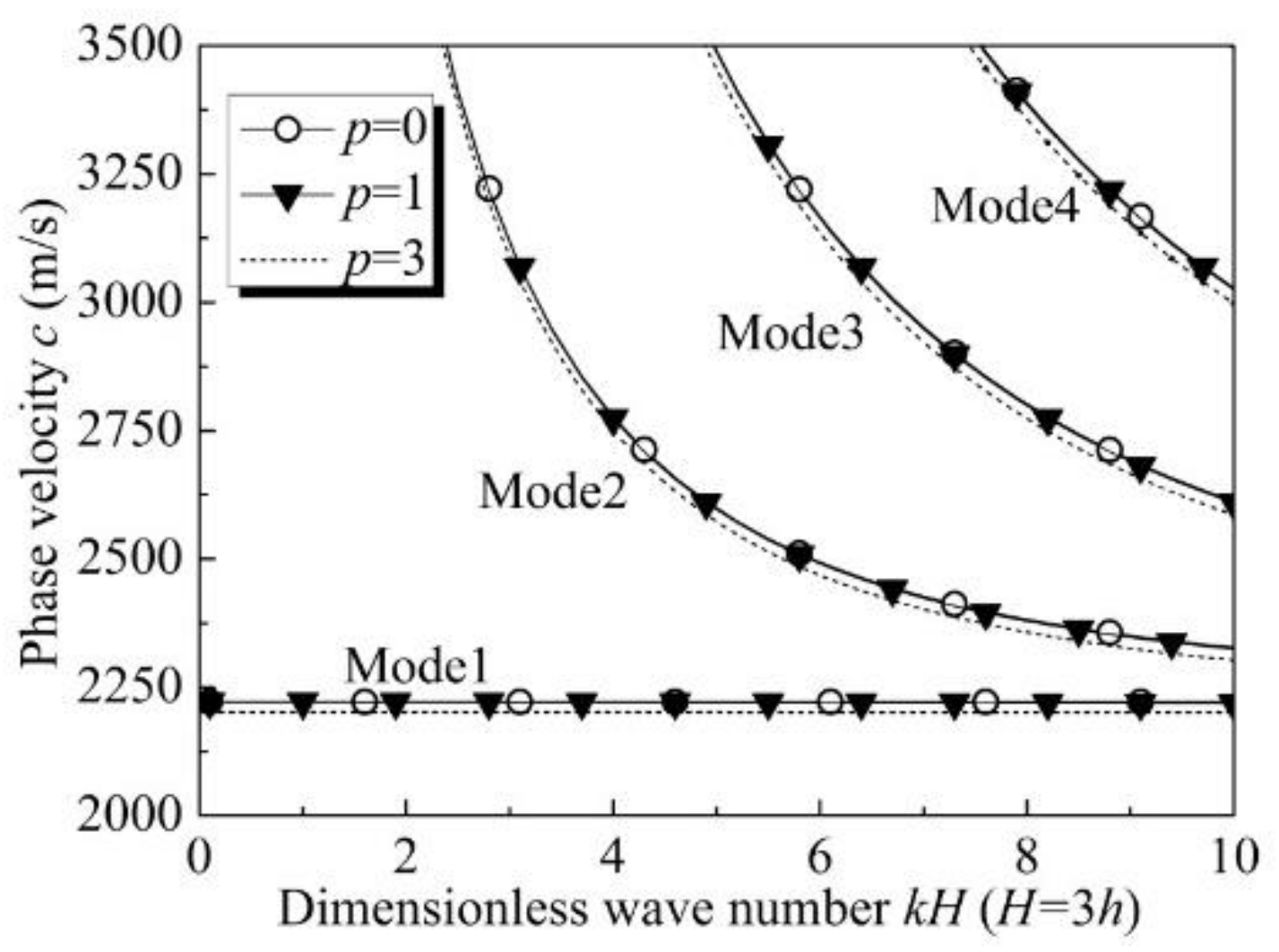
The dispersion curves of the Lamb waves in a three-layer wafer are calculated (Figure 7). Numerous modes of Lamb wave propagation exist in a multilayered FG nano copper wafer. The dispersion curves are similar to that of a simple FG nano copper wafer. For each mode, the larger the value of p, the smaller the phase velocity. The dispersion curves for and almost coincide, and the phase velocity at slightly decreases. To provide a theoretical basis for nondestructive evaluation, the variations of the change and relative change rate of the phase velocity with p at are plotted in Figure 8a,b, respectively.
When the thickness of the wafer is equal to the wavelength, the absolute values of the change in phase velocity and the relative change rate increase with the increase in p. If the wafer thickness is 5 mm and p is 3, the absolute values of the change in phase velocity for the first four modes are 8.349, 6.503, 10.839, and 25.781 m/s, respectively. The frequencies of Lamb waves with a given wavelength vary with different phase velocities. The frequency reduction is defined as , and the frequency reduction values for the first four modes are 3497.23, 2723.97, 4540.24, and 10,799.15 Hz, respectively. Although the relative variable of phase velocity is limited to less than 1.2% (Figure 8b), the absolute value of the frequency change is expressed in kilohertz. The gradient properties lead to the significant changes in frequency. The most obvious phase velocity change with the gradient parameters is observed in Mode 4, followed by Modes 3, 1, and 2 (Figure 8a). The values of Modes 1 and 3 almost coincide, whereas those of Modes 4 and 2 are the largest and lowest values among the four, respectively.
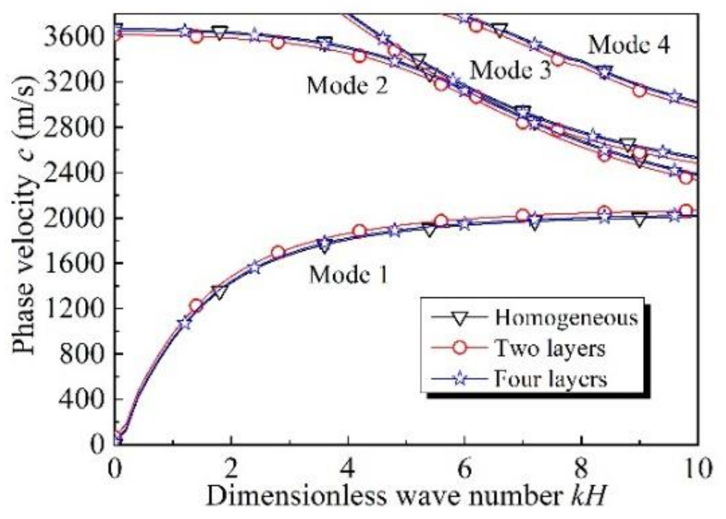
To reveal the Lamb wave properties in a multilayered FG nano copper wafer, the Lamb waves in an effective homogenous wafer are selected for comparison. The material parameters of the latter, which are selected as the average material parameters of the FG nano copper wafer, satisfy the following conditions.
where and are the Lamé coefficients and is the mass density of the effective homogenous wafer. At ,
The dispersion curves of the first four modes of the two-layer, four-layer, and effective homogenous wafers are displayed in Figure 9. The dispersion curve of the four-layer FG nano copper wafer is closer to the curve of the effective homogenous wafer than that of the two-layer FG nano copper wafer. The findings suggest the difference in the Lamb wave propagation in a multilayered FG nano copper wafer weakens with the increase in the number of layers.
5. Conclusions
In this study, Lamb waves’ propagation in an FG nano copper single wafer and in an FG nano copper layered wafer are investigated analytically. The power series method is employed for solving the ordinary differential equations with variable coefficients. The modified transfer matrix method based on the power series solution is then proposed to solve the wave propagation problem in a multilayered wafer. Compared with the Lamb waves in a regular homogenous copper wafer, those in the FG nano copper lead to the decreased in phase velocity. It can be obtained from the theoretical results that the gradient coefficients can be measured by using the change of phase velocity of Lamb waves. For both a single layer structure and a multilayered structure, the findings show that the variation in the phase velocity in Mode 2 is the least obvious among the four modes considered in the analysis, whereas that in Mode 4 is the most obvious. Therefore, Mode 4 is recommended to be used in nondestructive evaluation. For a multilayered FG nano copper wafer, if the number of layers is greater than four, the dispersion curves of the Lamb waves in this structure tend to coincide with those in an effective homogeneous structure. It is suggested that Lamb waves’ technique is not suitable for testing a multilayered FG nano copper wafer in which the number of sub-layers is larger than four. These results provide theoretical guidance for the nondestructive evaluation of FG nano layered structures.
Author Contributions
Conceptualization, X.C.; data curation, Y.H. and Y.N.; funding acquisition, Y.H., X.C. and Y.R., J.S.; methodology, X.C. and Y.R.; software, X.C. and Y.N.; supervision, X.C.; Writing—original draft, Y.H., X.C. and Y.R.; writing—review and editing, X.C. and J.S. All authors have read and agreed to the published version of the manuscript.
Funding
This research was supported by the National Natural Science Foundation of China (Nos. 11972285, 11572244, 11872300). It is also supported by the Natural Science Foundation of Shannxi Province, China (No. 2021JZ-47, 2021JQ-467) and NSAF (No. U1630144) and the Youth Innovation Team of Shaanxi Universities.
Conflicts of Interest
The authors declare no conflict of interest.
References
- Fang, T.H.; Li, W.L.; Tao, N.R.; Lu, K. Revealing extraordinary intrinsic tensile plasticity in gradient nano-grained copper. Science 2011, 331, 1587–1590. [Google Scholar] [CrossRef] [PubMed] [Green Version]
- Lu, K. Making strong nanomaterials ductile with gradients. Science 2014, 345, 1455–1456. [Google Scholar] [CrossRef] [PubMed]
- Thevamaran, R.; Lawal, O.; Yazdi, S.; Jeon, S.-J.; Lee, J.-H.; Thomas, E.L. Dynamic creation and evolution of gradient nanostructure in single-crystal metallic microcubes. Science 2016, 354, 312–316. [Google Scholar] [CrossRef] [PubMed]
- Yang, L.; Tao, N.R.; Lu, K.; Lu, L. Enhanced fatigue resistance of Cu with a gradient nanograined surface layer. Scr. Mater. 2013, 68, 801–804. [Google Scholar] [CrossRef]
- Yang, D.K.; Cizek, P.; Fabijanic, D.; Wang, J.T.; Hodgson, P.D. Work hardening in ultrafine-grained titanium: Multilayering and grading. Acta Mater. 2013, 61, 2840–2852. [Google Scholar] [CrossRef]
- Wang, Q.; Yin, Y.; Sun, Q.; Xiao, L.; Sun, J. Gradient nano microstructure and its formation mechanism in pure titanium produced by surface rolling treatment. J. Mater. Res. 2014, 29, 569–577. [Google Scholar] [CrossRef]
- Yuan, C.; Fu, R.; Sang, D.; Yao, Y.; Zhang, X. The tensile properties and fracture behavior of gradient nano-grained/coarse-grained zirconium. Mater. Lett. 2013, 107, 134–137. [Google Scholar] [CrossRef]
- Lu, X.L.; Lu, Q.H.; Li, Y.; Lu, L. Gradient confinement induced uniform tensile ductility in metallic glass. Sci. Rep. 2013, 3, 3319. [Google Scholar] [CrossRef]
- Wang, H.T.; Tao, N.R.; Lu, K. Architectured surface layer with a gradient nanotwinned structure in a Fe-Mn austenitic steel. Scr. Mater. 2013, 68, 22–27. [Google Scholar] [CrossRef]
- Moering, J.; Ma, X.; Chen, G.; Miao, P.; Li, G.; Qian, G.; Mathaudhu, S.; Zhu, Y. The role of shear strain on texture and microstructural gradients in low carbon steel processed by Surface Mechanical Attrition Treatment. Scr. Mater. 2015, 108, 100–103. [Google Scholar] [CrossRef] [Green Version]
- Zhao, J.; Xia, W.; Li, N.; Li, F.-L. A gradient nano/micro-structured surface layer on copper induced by severe plasticity roller burnishing. Trans. Nonferrous Met. Soc. China 2014, 24, 441–448. [Google Scholar] [CrossRef]
- Wang, Y.L.; Molotnikov, A.; Diez, M.; Lapovok, R.; Kim, H.; Wang, J.T.; Estrin, Y. Gradient structure produced by three roll planetary milling: Numerical simulation and microstructural observations. Mater. Sci. Eng. A Struct. Mater. Prop. Microstruct. Process. 2015, 639, 165–172. [Google Scholar] [CrossRef]
- Yin, Z.; Yang, X.; Ma, X.; Moering, J.; Yang, J.; Gong, Y.; Zhu, Y.; Zhu, X. Strength and ductility of gradient structured copper obtained by surface mechanical attrition treatment. Mater Des. 2016, 105, 89–95. [Google Scholar] [CrossRef]
- Zeng, Z.; Li, X.; Xu, D.; Lu, L.; Gao, H.; Zhu, T. Gradient plasticity in gradient nano-grained metals. Extrem. Mech. Lett. 2016, 8, 213–219. [Google Scholar] [CrossRef] [Green Version]
- Rose, J.L. Ultrasonic Waves in Solid Media; Cambridge University Press: Cambridge, MA, USA, 1999. [Google Scholar]
- Achenbach, J.D. Wave Propagation in Elastic Solids; Elsevier: New York, NY, USA, 1984. [Google Scholar]
- Wang, J.; Du, J. A two-dimensional analysis of surface acoustic waves in finite elastic plates with eigensolutions. Sci. China Phys. Mech. Astron. 2007, 50, 631–649. [Google Scholar] [CrossRef]
- Du, J.; Jin, X.; Wang, J.; Xian, K. Love wave propagation in functionally graded piezoelectric material layer. Ultrasonics 2007, 46, 13–22. [Google Scholar] [CrossRef]
- Collet, B.; Destrade, M.; Maugin, G.A. Bleustein-Gulyaev waves in some functionally graded materials. Eur. J. Mech. A Solids 2006, 25, 695–706. [Google Scholar] [CrossRef] [Green Version]
- Cao, X.; Jin, F.; Wang, Z. Theoretical investigation on horizontally shear waves in a functionally gradient piezoelectric material plate. In Proceedings of the 7th International Conference on Fracture and Strength of Solids, FEOFS 2007, Urumqi, China, 27–29 August 2007; pp. 707–712. [Google Scholar]
- Vlasie, V.; Rousseau, M. Guided modes in a plane elastic layer with gradually continuous acoustic properties. NDT E Int. 2004, 37, 633–644. [Google Scholar] [CrossRef]
- Qian, Z.H.; Jin, F.; Lu, T.; Hirose, S. Transverse surface waves in a piezoelectric material carrying a gradient metal layer of finite thickness. Int. J. Eng. Sci. 2009, 47, 1049–1054. [Google Scholar] [CrossRef]
- Li, X.Y.; Wang, Z.K.; Huang, S.H. Love waves in functionally graded piezoelectric materials. Int. J. Solids Struct. 2004, 41, 7309–7328. [Google Scholar] [CrossRef]
- Lefebvre, J.E.; Zhang, V.; Gazalet, J.; Gryba, T.; Sadaune, V. Acoustic wave propagation in continuous functionally graded plates: An extension of the Legendre polynomial approach. Ieee Trans. Ultrason. Ferroelectr. Freq. Control 2001, 48, 1332–1340. [Google Scholar] [CrossRef] [PubMed]
- Yu, J.G.; Zhang, C. Effects of initial stress on guided waves in orthotropic functionally graded plates. Appl. Math. Model. 2014, 38, 464–478. [Google Scholar] [CrossRef]
- Yu, J.G.; Wu, B.; He, C.F. Guided thermoelastic waves in functionally graded plates with two relaxation times. Int. J. Eng. Sci. 2010, 48, 1709–1720. [Google Scholar] [CrossRef]
- Cao, X.; Jin, F.; Jeon, I. Calculation of propagation properties of Lamb waves in a functionally graded material (FGM) plate by power series technique. Ndt E Int. 2011, 44, 84–92. [Google Scholar] [CrossRef]
- Yan, L.; Zhang, J.; Song, G.; Liu, M.; He, C. The dispersion curves and wave structures of Lamb waves in functionally graded plate: Theoretical and simulation analysis. In Proceedings of the 45th Annual Review of Progress in Quantitative Nondestructive Evaluation; Bond, L.J., Holland, S., Laflamme, S., Eds.; AIP Publishing LLC: Burlington, VT, USA, 2019; Volume 2102, p. 050020. [Google Scholar]
- Liu, C.; Yu, J.; Xu, W.; Zhang, X.; Wang, X. Dispersion characteristics of guided waves in functionally graded anisotropic micro/nano-plates based on the modified couple stress theory. Thin Walled Struct. 2021, 161, 107527. [Google Scholar] [CrossRef]
- Liu, C.; Yu, J.; Zhang, B.; Zhang, X.; Elmaimouni, L. Analysis of Lamb wave propagation in a functionally graded piezoelectric small-scale plate based on the modified couple stress theory. Compos. Struct. 2021, 265, 113733. [Google Scholar] [CrossRef]
- Tani, J.; Liu, G.R. SH surface waves in functionally gradient piezoelectric plates. JSME Int. J. Ser. AMech. Mater. Eng. 1993, 36, 152–155. [Google Scholar] [CrossRef] [Green Version]
- Liu, G.R.; Tani, J.; Ohyoshi, T.; Watanabe, K. Characteristic wave surfaces in anisotropic laminated plates. ASME J. Vib. Acoust. 1991, 113, 279–285. [Google Scholar] [CrossRef]
- Liu, G.R.; Dai, K.Y.; Han, X.; Ohyoshi, T. Dispersion of waves and characteristic wave surfaces in functionally graded piezoelectric plates. J. Sound Vib. 2003, 268, 131–147. [Google Scholar] [CrossRef]
- Yang, J.; Yang, Z. Analytical and numerical modeling of resonant piezoelectric devices in China—A review. Sci. China Ser. G Phys. Mech. Astron. 2008, 51, 1775–1807. [Google Scholar] [CrossRef]
- Golub, M.V.; Fomenko, S.I.; Bui, T.Q.; Zhang, C.; Wang, Y.S. Transmission and band gaps of elastic SH waves in functionally graded periodic laminates. Int. J. Solids Struct. 2012, 49, 344–354. [Google Scholar] [CrossRef] [Green Version]
- Fomenko, S.I.; Golub, M.V.; Zhang, C.; Bui, T.Q.; Wang, Y.S. In-plane elastic wave propagation and band-gaps in layered functionally graded phononic crystals. Int. J. Solids Struct. 2014, 51, 2491–2503. [Google Scholar] [CrossRef] [Green Version]
- Kuznetsov, S.V. Abnormal dispersion of flexural Lamb waves in functionally graded plates. Z. Für Angew. Math. Und Phys. Zamp 2019, 70, 89. [Google Scholar] [CrossRef]
- Kuznetsov, S.V. Similarity and discrepancy of Lamb wave propagation in functionally graded, stratified, and homogeneous media. Int. J. Dyn. Control 2020, 8, 717–722. [Google Scholar] [CrossRef]
- Hu, Y.; Cao, X.; Niu, Y.; Ru, Y. SH waves in a functionally graded nano copper layered wafer. In Proceedings of the 2019 14th Symposium on Piezoelectrcity, Acoustic Waves and Device Applications (SPAWDA), Shijiazhuang, China, 1–4 November 2019. [Google Scholar]
- Wang, G.F.; Feng, X.Q.; Yu, S.W. Interface effects on effective elastic moduli of nanocrystalline materials. Mater. Sci. Eng. A 2003, 363, 1–8. [Google Scholar] [CrossRef]
Figure 1.
Two types of FG nano copper wafer. (a) Simple FG nano copper wafer; (b) multi-layered FG nano copper wafer.
Figure 1.
Two types of FG nano copper wafer. (a) Simple FG nano copper wafer; (b) multi-layered FG nano copper wafer.

Figure 2.
Microstructure model of nanocrystalline materials [40].
Figure 2.
Microstructure model of nanocrystalline materials [40].

Figure 3.
Variations of the material parameters with thickness for different p values: (a) grain size, (b) λ, (c) μ, and (d) ρ.
Figure 3.
Variations of the material parameters with thickness for different p values: (a) grain size, (b) λ, (c) μ, and (d) ρ.


Figure 4.
Variations of the material parameters of a three-layer structure with thickness for different p values: (a) grain size, (b) λ, (c) μ, and (d) ρ.
Figure 4.
Variations of the material parameters of a three-layer structure with thickness for different p values: (a) grain size, (b) λ, (c) μ, and (d) ρ.

Figure 5.
Dispersion curves of Lamb waves in a single FG nano copper wafer.

Figure 6.
Relationship between the change in phase velocity and p in a simple FG nano cooper wafer: (a) change in phase velocity and (b) relative change rate of the phase velocity.
Figure 6.
Relationship between the change in phase velocity and p in a simple FG nano cooper wafer: (a) change in phase velocity and (b) relative change rate of the phase velocity.

Figure 7.
Dispersion curves of the Lamb waves in a three-layer FG nano cooper wafer.

Figure 8.
Relationship between the change in phase velocity and p in a three-layer FG nano cooper wafer: (a) change in phase velocity and (b) relative change rate of the phase velocity.
Figure 8.
Relationship between the change in phase velocity and p in a three-layer FG nano cooper wafer: (a) change in phase velocity and (b) relative change rate of the phase velocity.

Figure 9.
Dispersion curves of the Lamb waves in a two-layer, four-layer, and effective homogenous wafers.
Figure 9.
Dispersion curves of the Lamb waves in a two-layer, four-layer, and effective homogenous wafers.

Publisher’s Note: MDPI stays neutral with regard to jurisdictional claims in published maps and institutional affiliations. |
© 2021 by the authors. Licensee MDPI, Basel, Switzerland. This article is an open access article distributed under the terms and conditions of the Creative Commons Attribution (CC BY) license (https://creativecommons.org/licenses/by/4.0/).
Share and Cite
MDPI and ACS Style
Hu, Y.; Cao, X.; Niu, Y.; Ru, Y.; Shi, J. Asymptotic Analytical Solution on Lamb Waves in Functionally Graded Nano Copper Layered Wafer. Appl. Sci. 2021, 11, 4442. https://doi.org/10.3390/app11104442
AMA Style
Hu Y, Cao X, Niu Y, Ru Y, Shi J. Asymptotic Analytical Solution on Lamb Waves in Functionally Graded Nano Copper Layered Wafer. Applied Sciences. 2021; 11(10):4442. https://doi.org/10.3390/app11104442
Chicago/Turabian StyleHu, Yifeng, Xiaoshan Cao, Yi Niu, Yan Ru, and Junping Shi. 2021. "Asymptotic Analytical Solution on Lamb Waves in Functionally Graded Nano Copper Layered Wafer" Applied Sciences 11, no. 10: 4442. https://doi.org/10.3390/app11104442
Note that from the first issue of 2016, this journal uses article numbers instead of page numbers. See further details here.