The Steelmaking Process Parameter Optimization with a Surrogate Model Based on Convolutional Neural Networks and the Firefly Algorithm

Abstract

High-strength low-alloy steels (HSLAs) are widely used in the structural body components of many domestic motor vehicles owing to their better mechanical properties and greater resistance. The real production process of HSLA steelmaking can be regarded as a model that builds on the relationship between process parameters and product quality attributes. A surrogate modeling method is used, and the resulting production process model can be applied to predict the optimal manufacturing process parameters. We used different methods in this paper, including linear regression, random forests, support vector regression, multilayer perception, and a simplified VGG model to build such a surrogate model. We then applied three bio-inspired search algorithms, namely particle swarm optimization, the artificial bee colony algorithm, and the firefly algorithm, to search for the optimal controllable manufacturing process parameters. Through experiments on 9000 test samples used for building the surrogate model and 299 test samples for making the optimal process parameter selection, we found that the combination of a simplified VGG model and the firefly algorithm was the most successful at reaching a success rate of 100%—in other words, when the product quality attributes of all test samples satisfy the mechanical requirements of the end products.

1. Introduction

Under the pressure of the fierce competition between steel companies, quality improvements in high-strength low-alloy steel (HSLA) products are constantly being pursued. Abnormal variations in upstream process parameters such as alloy composition might cause deviations in mechanical properties and thus lead to unsatisfactory quality and a high rejection rate. To reduce the rejection rate and to effectively improve the competitiveness of China Steel Corporation (CSC) products, we developed a dynamic process control system to predict and monitor the mechanical properties of products before they enter downstream production lines. If the predicted mechanical properties deviate too much from the usual level, the system can perform quality compensation by calculating and applying appropriate downstream process parameters and thereby meet the final quality requirements. This is done through a sequence of up- and downstream production lines, which include the crude making, hot rolling, cold rolling, and cold-rolled coating lines. Each line should meet quality-level requirements, or else the overall finished products will not achieve their required qualities. In the crude making process, iron ore is first reduced to iron by mixing it with coal/coke and limestone in a blast furnace (BF); then, the iron is converted into steel using a basic oxygen furnace (BOF). The hot-rolling is a mill process in which the steel is rolled at a temperature above its recrystallization temperature. When steel is heated past its recrystallization point, it becomes more malleable and can be properly formed and shaped. This also allows for the 2.1ability to produce larger quantities of steel. The steel is then cooled at room temperature, which “normalizes” it, eliminating the worry for stresses in the material arising when quenching or work-hardening. Cold-rolling steel allows for the creation of precise shapes. Since the process is performed at room temperature, the steel will not shrink as it cools, as it does in the hot-rolled process. The cold-rolled use plastic coating to protect the steel surface.

Although the CSC is a high-quality manufacturer of HSLA, a small number of non-conforming products cause a great loss of finance and reputation. The steeling process parameter optimization is important to promote the quality of HSLA. Most manufacturing processes [1,2] require parameterization to achieve their optimal cost, quality, and other properties. The number of process parameters considered usually exceeds 10 or even 100, and current approaches to their optimization require many expensive and complex experiments. Although some physically precise simulation models have been developed, such as the finite element method [3] and the Taguchi method [4], these need many hours or even days for computation. Another approach is the use of surrogate models, which can effectively decrease the number of simulations needed when applied to the problems of process parameter optimization.

The surrogate model is an easy-to-evaluate approach to construct high-fidelity product models [5,6,7,8,9], which were created by using a decision tree, artificial neural network, radial basis function, kernel smoothing, and stochastic processes [10]. Surrogate-based optimization tries to search for the optimal process parameters based on an established surrogate model, and it requires an appropriate mechanism to do so. Genetic algorithms [11] and model-based self-optimizations [12] have been used to iteratively improve candidate process parameters.

Machine learning methods have been widely used in materials design and engineering, such as the predictive maintenance of anodes [13], casting steel [14], and the prediction of the steel’s properties [15]. In this paper, we use different methods to build surrogate models for steelmaking process parameter optimization. These methods include linear regression (LR), random forests (RF) [16], support vector regression (SVR) [17], artificial neural networks (ANNs) [18,19,20,21], and convolutional neural networks (CNNs) [22]. In addition, we use three different bio-inspired search algorithms—particle swarm optimization (PSO) [23], the artificial bee colony (ABC) algorithm [24], and the firefly algorithm (FA) [25]—to search for optimal process parameters.

We further developed a simplified 1D version of the original 2D Visual Geometry Group (VGG) 16 model [26,27] to establish a surrogate model between the process parameters and the product quality attributes, as shown in Figure 1. This 1D VGG model is called the simplified VGG (SVGG) model, and it can be regarded as a process for controlling HSLA product quality attributes through its parameter inputs.

Figure 1. Surrogate model.

To meet the product quality requirements of HSLA, we applied the PSO, ABC, and firefly algorithm to search for the optimal adjustable process parameters and then compare their performance. In our experiments, 9000 samples (meeting the quality requirements) were used to train the five different methods for establishing the surrogate model, and 299 samples (not meeting the quality requirements) were used to evaluate three bio-inspired process optimization search algorithms. The FA ultimately produced the most optimal selection of adjustable process parameters. Our experimental results further showed that all the adjustable process parameters used in our test samples were successful in determining whether the corresponding product attributes met the mechanical requirements of the product.

The main contributions of this paper are as follows:

• We addressed the interesting problem of steelmaking process parameter optimization by proposing a simplified VGG model to build a surrogate model and then compared it with four other machine-learning methods.
• We applied three different algorithms—PSO, the ABC, and the FA—to search for optimal process parameters and then evaluated their performance. Our experimental results demonstrated that the FA can achieve high performance and outperforms the other methods.

The remainder of this paper is organized as follows. Section 2 reviews the machine-learning methods and bio-inspired algorithms. Section 3 describes our proposed method called the simplified VGG model + Firefly algorithm to search for optimal process parameters. Section 4 presents our experimental results and discussions. Finally, conclusions and remarks are given in Section 5.

2. Related Works

2.1. Surrogate Model

A production process can be represented as a function $\pi :X\to Y$, in which X denotes the process parameters, and Y denotes the product attributes. This function maps process parameter configurations $x\in X$ to product attributes $y\in Y.$, and the map can be regarded as a surrogate model $\phi :X\to Y$ based on all observations (X_i, Y_i). The construction of a surrogate model needs a fitness function to evaluate how well the model predictions match the observations. In general, we need an optimizer to obtain the optimal linear or nonlinear maps. In this study, we use linear regression, random forests, support vector regression, neural networks, and convolutional neural networks to build surrogate models, with process parameter optimization being dependent on the accuracy of these models. These five methods are described in the following subsections.

2.2. Survey of Machine Learning Method

2.2.1. Linear Regression

Linear regression (LR) is a simple and attractive method for building a surrogate model, as based on Equation (1):

$$Y_j={\alpha }_{1,j}{f}_1+{\alpha }_{2,j}{f}_2+{\alpha }_{3,j}{f}_3+\dots +{\alpha }_{30,j}{f}_{30}+{\beta }_j$$

(1)

where $Y_j$ and $f_i$ are the j-th product attribute and the i-th dimension of the process parameters, respectively. Particularly, the gradient descent method is used to decide the regression parameters ${\alpha }_{i,j} \mathrm{and} {\beta }_j$.

2.2.2. Random Forests

Random forests (RFs) is an ensemble learning method used for classification or regression that constructs a multitude of decision trees at training time and outputs the mode or mean predictions of those individual trees. In general, RFs outperform traditional decision tree methods because they can overcome the problem of overfitting. In the implementation of an RF algorithm, new training sample sets are randomly selected by replacing the original training set. Each training set is separated into two in-of-bag sets, including one-third of the samples and one out-of-bag set from the remaining two-thirds of the samples. All samples in the out-of-bag set are collected into test samples, while samples from each of the in-of-bag sets are dependently built by decision tree induction into their own decision tree. This way, the regression results R($x_i$) of each test sample $x_i$ are calculated by Equation (2):

$$R\left(x_i\right)=\frac{1}{M}{{\displaystyle \sum }}_{m=1}^M{y}_m$$

(2)

where M is the number of decision trees, and $y_m$ is the decision value of the m-th decision tree of test sample $x_i.$

2.2.3. Support Vector Regression

Support vector machines are intelligent statistical learning algorithms used for classification and regression. They solve regression problems through a nonlinear mapping function $\mu \left(x_i\right)$, which maps the original samples x_i to a feature space of a higher dimension, and then uses the linear regression method to compute the corresponding targets. Given a set of n training data {$\left(x_1,y_1\right),\left(x_2,y_2\right),\left(x_3,y_3\right),\dots .,\left(x_n,y_n\right)\}\in R^n\times R$, where $x_i$ is the input vector and $y_i$ is its target, the following decision function can be defined:

$$f\left(x\right)=\omega ·\mu \left(x_i\right)+b$$

(3)

where $·$ is the inner product, ω is the weight vector, and b is the bias parameter.

SVR applies the structured risk minimization principle to generate the above decision function [see Equation (3)] by minimizing a regularized risk function as presented in Equations (4) and (5):

$$\mathrm{Regularized} \mathrm{risk}=\frac{C}{n}{{\displaystyle \sum }}_{i=1}^{n}L\left(y_i,f\left(x_i\right)\right)+\frac{1}{2}{||\omega ||}^2$$

(4)

where:

$$L\left(y_i,f\left(x_i\right)\right)=\left\{\begin{array}{c}\left|y_i-f\left(x_i\right)\right|\\ 0\end{array}\right.,\hspace{0.33em}\begin{array}{c}if\left|y_i-f\left(x_i\right)\right|\ge \epsilon \\ otherwise\end{array}$$

(5)

In SVR, Vapnik’s ε-insensitive loss function is used to measure empirical risk, where ε is the tube size, $\frac{1}{2}{||\omega ||}^2$ is a regularization term used as a measure of flatness or complexity of the function, and C is a regularized constant that describes the trade-off between the empirical risk and the regularization term.

According to Wolfe duality and the saddle-point condition, the dual optimization problem of the aforementioned primal one is described by the following term:

$$\begin{array}{c}max\\ \alpha ,{\alpha }^{*}\end{array}(-\frac{1}{2}{\displaystyle \sum }_{i,j=1}^n\left({\alpha }_i-{\alpha }_i^{*}\right)\left({\alpha }_j-{\alpha }_j^{*}\right)), \mathrm{s}.\mathrm{t}.{\displaystyle \sum }_{i,j=1}^n\left({\alpha }_i-{\alpha }_i^{*}\right)=0,{\alpha }_i,{\alpha }_i^{*}\in \left[0, C\right]$$

(6)

The weight parameters are then described by $w={{\displaystyle \sum }}_{i=1}^n\left({\alpha }_i-{\alpha }_i^{*}\right)\mu \left(x_i\right)$, where ${\alpha }_i\mathrm{and}{\alpha }_i^{*}$ are nonnegative Lagrange multipliers, which can be obtained to solve the convex quadratic programming. Finally, based on Equation (7) and the radial basis function (RBF) kernel trick, the decision function given by Equation (3) has the following specific form:

$$f\left(x\right)={{\displaystyle \sum }}_i^n\left({\alpha }_i-{\alpha }_i^{*}\right)e^{\frac{-{\left|x_i-x_j\right|}^2}{2{\sigma }^2}}+b$$

(7)

where,

$$b=y_j-{\displaystyle \sum }_{i=1}^n{y}_i{\alpha }_i^{*}{e}^{\frac{-{\left|x_i-x_j\right|}^2}{2{\sigma }^2}}$$

(8)

with σ representing the kernel parameters and $j\in \{j$ < C}. Note, there are three penalty parameters: C, the RBF kernel parameter, and the width of the ε loss function.

2.2.4. Multilayer Perception

Multilayer perception (MLP) is a powerful class of data-driven function approximation algorithms that represent information through a hierarchy of features. They follow a simple ANN model, beginning with the input layer and ending with the final output layer, with intermediate layers known as hidden layers. By manipulating the number of hidden layers and the size of each, one can learn functions of arbitrary complexity. The input and output layer sizes are fixed, being determined by the dimensionality of the input feature and the output target. Except for the input nodes, each node is a neuron that uses a nonlinear activation function. MLP algorithms also utilize a supervised learning technique, i.e., backpropagation for training. We used an MLP algorithm with two hidden layers; each one has 100 nodes, the dimension of the input layer is 30 (the dimension of our process parameters) and involves three targets (the product attributes).

2.3. Bio-Inspired Search Algorithms

Over the last decade, modeling the behavior of social insects such as ants and bees has been used as a way of solving search problems. There are many different bio-inspired search algorithms, including particle swarm optimization, artificial bee colony, and the firefly algorithm, which have been widely used in numerical optimization [28], motion estimation [29], image thresholding [30,31], neural network parameter training [32], enhanced near field characteristic [33], simulation-driven spatial phase shifters [34], and electromagnetic band-gap resonator antenna [35].

2.3.1. Particle Swarm Optimization

Particle swarm optimization (PSO) is a metaheuristic, stochastic, and population-based evolutionary optimization algorithm, and its standard form was initially developed by Kennedy Eberhart [36]. It searches for an optimal solution in its search space through the modeling of a swarm, where each particle in the swarm survives with a velocity and a position in the solution search space. The lower and upper bounds of each dimension of a particle are denoted in the algorithm by lb and ub. It improves on the best solution traversed so far by iteratively updating its velocity and position in the search space, as described by Equations (9) and (10):

$$v_i\left(t+1\right)=\omega v_i\left(t\right)+c_1{r}_1(p_i\left(t\right)-x_i\left(t\right)+c_2{r}_2\left(p_g\left(t\right)-x_i\left(t\right)\right)$$

(9)

$$x_i\left(t+1\right)=x_i\left(t\right)+v_i(\mathrm{t}+1)$$

(10)

where ω indicates the inertia weight, $c_1$ and $c_2$ are the learning rates, $r_1$ and $r_2$ are random numbers ranging from 0 to 1, and $p_i\left(t\right)$ and $p_g\left(t\right)$ represent the personal local best and the global best, respectively.

2.3.2. Artificial Bee Colony Algorithm

The artificial bee colony (ABC) algorithm, as proposed by Karaboga and Basturk [37], has recently become available and is a promising technique for solving real-world optimization problems. It models a colony of artificial bees, containing three different groups: employed bees, onlookers, and scouts. The employed bees carry information about food sources and share it in the dancing area of the hive. The onlookers wait in the dancing area to receive this probability information from the employed bees, and they use it to make decisions regarding the selection of a food source. The computation of this probability is based on the amount of food located at each source. The other kind of bee—scouts carries out random searches for new food sources. An employed bee becomes a scout when its food source is abandoned and becomes an employed bee again as soon as it finds a new food source. Therefore, each cycle of the ABC algorithm contains three steps. First, employed bees are sent to the known food sources, and the amounts of nectar are calculated. After receiving that information, onlooker bees visit the food sources and provide updates. When the nectar at a food source is depleted, a scout is sent out to find a new food source.

Within the algorithm, the position of a food source $x_i$ represents a candidate solution to the optimization problem, and the amount of nectar at this food source is denoted as its fitness (fit). In general, the number of employed bees or onlookers is equal to the number of food sources. Initially, the ABC algorithm randomly generates a distributed initial population of K solutions, denoted by $P=\left\{x_{1,}{x}_2,\dots ,x_K\right\}$, where K denotes the number of employed bees or onlookers, and each solution $x_i$ (for i = 1, 2,…, K) is a D-dimensional vector. During each execution cycle C (where C = 1, 2,…, MCN, the maximum cycle number), the population of solutions is subjected to the search processes of the employed bees, onlookers, and scouts. An employed bee modifies the possible solution as a function of the fitness value (amount of nectar) of the new solution (food source) by using Equation (11):

$$v_{ij}=x_{ij}+\phi (x_{ij}-x_{kj})$$

(11)

where $k\in \{1,2,\dots ,K$}, but $k\ne I$ and $j\in \left\{1,2,\dots ,D\right\}$ are randomly selected indexes, and φ is a random number between −1 and 1.

If the fitness value of the new solution $v_i$ is greater than that of the previous solution $x_i$, then the employed bee simultaneously remembers the new solution and abandons the old one; otherwise, it will retain the location of the old one in its memory.

When all employed bees have finished their search process, they bring back the information they have on the positions and nectar amounts of all food sources to the onlookers. Each of the onlookers then decides on a particular food source to further call upon, according to a probability proportional to the amount of nectar at that food source. This probability $p_i$ of selecting a food source $z_i$ is determined using the following Equation (12):

$$p_i=\frac{fit\left(z_i\right)}{{{\displaystyle \sum }}_{n=1}^{K}fit\left(z_n\right)}$$

(12)

In practice, each food source $z_i$ sequentially generates a random number between 0 and 1. If this random number is less than the probability $p_i$, an onlooker is sent to the food source and produces a new solution based on Equation (13):

$$v_{ij}=z_{ij}+\phi (z_{ij}-z_{kj})$$

(13)

where $k\in \{1,2,\dots ,K$}, but $k\ne i$ and $j\in \left\{1,2,\dots ,D\right\}$ are randomly selected indexes, and φ is a random number between −1 and 1.

If the fitness value of the new solution is greater than the old one, the onlooker memorizes the new solution and shares this information with the other onlookers. Otherwise, the new solution is discarded. This process is repeated until all onlookers have been distributed to food sources. If the food source could be improved upon (as predetermined by a limiting value), then it is abandoned, and the corresponding employed bee becomes a scout. This scout then goes on to discover a new food source to replace $theabandonedsolution{z}_j$, as described by Equation (14):

$$z_{ij}=z_{min}^j+\sigma \left(z_{max}^j-z_{min}^j\right)$$

(14)

where $z_{min}^j$ and $z_{max}^j$ are the lower and upper bounds of the j-th component of the solution, and σ is a random number ranging from −1 to 1. If the new solution is better than the $abandonedsolution{z}_j$, the scout becomes an employed bee, and the new solution is retained.

The search processes of the employed, onlooker, and scout bees are repeated until the execution cycle equals MCN. Of all the methods described so far, the best solutions with the largest fitness are outputted by this ABC algorithm.

2.3.3. Firefly Algorithm

The firefly algorithm (FA) was developed by Xin-She Yang at Cambridge University in 2008 [38,39,40,41]. It has three idealized rules: first, all fireflies are unisex, so each firefly is attracted to all other fireflies, regardless of their sex. Second, attractiveness is proportional to brightness—thus, for any two flashing fireflies, the least bright one will move toward the brighter one. If there is no brighter one, then that particular firefly will move randomly. To model firefly attractiveness, one should select any monotonically decreasing function of the distance $r_{i,j}=d\left(x_j,x_i\right)$ from the chosen (j-th) firefly $x_j$ to the target (i-th) firefly $x_i$. This is described by Equations (15) and (16):

$$r_{i,j}=||x_i-x_j||$$

(15)

$$\beta \leftarrow {\beta }_0{e}^{-\gamma r_{i,j}}$$

(16)

where ${\beta }_0$ is the attractiveness at $r_{i,j}=0$, and γ is the light absorption coefficient at the source. The movement of firefly i when it is attracted to another, more attractive firefly j is determined by:

$$x_{i,k}\leftarrow \left(1-\beta \right)x_{i,k}+\beta x_{j,k}+u_{i,k}$$

(17)

$$u_{i,k}=\alpha \left(\mathrm{rand}1-\frac{1}{2}\right)$$

(18)

If a particular firefly $x_i$ is already the brightest (i.e., it is the one with the maximum fitness), then it will move randomly according to the following equations:

$$x_{i^{\max },k}\leftarrow x_{i^{\max },k}+u_{i^{\max },k}, k=1, 2,\dots , D$$

(19)

$$u_{i^{\max },k}=\alpha \left(\mathrm{rand}2-\frac{1}{2}\right)$$

(20)

where $\mathrm{rand}1\approx U\left(0,1\right)$ and $\mathrm{rand}2\approx U\left(0,1\right)$ are random numbers obtained from a uniform distribution.

The third rule is that the brightness of a firefly is affected or determined by the landscape of the fitness function $\phi \left(•\right)$. For maximization problems, the brightness I of a firefly at a particular location x can be chosen as a function I(x) that is proportional to the value of the fitness function $\phi \left(x\right)$.

3. Material and Methods

3.1. Materials and Experimental Setup

All experiments were performed on a PC with an Intel Core i5 3.30 GHz CPU, 8 GB of RAM, and an NVIDIA GeForce GTX 1060 GPU. All used machine-learning methods were implemented in simultaneously multitask learning and coded the programs by using Python language, and then individually were used to verify the performance of process parameters optimization using the four-fold cross-validation method.

The 9299 HSLA samples were collected from the China Steel Corporation (Kaohsiung, Taiwan) from 2016 to 2010. Each sample has a 30-dimensional process parameter and three corresponding product quality attributes., respectively. The 9299 samples included the 9000 training data samples (two of 10 samples as validation samples), which meets the quality requirement and 299 false samples (as test samples) of no meeting requirements. In general, the false samples are difficult to collect since the CSC is a high-quality steel manufacturer. Each process parameter x includes temperature, steeling time, iron composition, and so on. The product attribute Y includes three quality attributes, i.e., yield stress, tensile stress, and plastic strain ratio. The products of HSLA must meet reasonable quality ranges for these three attributes yield stress [0,185], tensile stress [270, $\infty$], and plastic strain ratio [39, $\infty$]. For easy identification, the process parameters are represented by x_i = (f_i1, f_i2,…, f_i30) for i = 1, 2,…, 9000, and the product attributes are represented by Y_i = (y_i1, y_i2, y_i3) for training samples. However, the additional 299 test samples have only 25 fixed process parameters, with the other five being adjustable parameters denoted by f_i2, f_i4, f_i6, f_i8, and f_i9 for the i-th test sample.

Table 1 shows the data for the five original training samples, where each includes the 30 dimensions of the process parameters, named $f_1$, $f_2$,…,$f_{30}$, and the three product attributes of $Y_1$, $Y_2$, and $Y_3$. The five adjustable process parameters are restricted to positive integers. In total, 9000 training samples were used to train the simplified VGG surrogate model, each including a complete set of process parameters and product attributes. However, five of the process parameters in each of the 299 test samples were adjustable.

Table 1. The X and Y is the sets of process parameters and product quality attributes. The X contains the parameters of temperature, steeling time, iron composition, and so on. The product attribute Y includes three quality attributes, i.e., yield stress, tensile stress, and plastic strain ratio.

Y1	Y2	Y3	X1	X2	X3	X4	X5	X6	X7	X8	X9	X10	X11	X12	X13	X14	X15	X16	X17	X18	X19	X20	X21	X22	X23	X24	X25	X26	X27	X28	X29	X30
148	294	49	758	752	582	411	363	318	282	134	83	923	640	4.002723	0.0021	0.15	0.013	0.006	0.01	0.004	0.01	0.02	0	0.001	0.0027	0.003	0.039	0.033	0.032	0.0001	0.001	0.0001
146	294	50	748	747	574	403	361	318	288	150	124	915	643	3.99594	0.0014	0.12	0.017	0.005	0.01	0.005	0.01	0.01	0	0.001	0.0018	0.002	0.04	0.03	0.029	0.0001	0.001	0.0001
176	309	47	751	757	575	397	351	318	285	195	80	924	640	3.19883	0.0024	0.15	0.015	0.003	0	0.005	0.01	0.02	0	0.001	0.0027	0.003	0.044	0.036	0.035	0.0001	0	0.0001
139	288	51	754	754	575	397	351	313	291	195	80	928	647	3.198287	0.0012	0.14	0.014	0.003	0	0.006	0.01	0.02	0	0	0.0014	0	0.046	0.037	0.034	0.0001	0	0.0001
145	299	48	777	772	564	404	367	324	296	216	80	920	641	3.198613	0.0017	0.15	0.015	0.003	0	0.006	0.01	0.02	0	0.001	0.0016	0.003	0.042	0.041	0.04	0.0001	0.001	0.0001
150	302	49	768	757	580	411	358	320	292	194	107	922	648	3.500751	0.0014	0.16	0.015	0.005	0.01	0.005	0.01	0.02	0	0.001	0.0015	0.003	0.042	0.035	0.034	0.0001	0.001	0.0001
166	310	47	749	752	572	405	364	326	293	200	100	925	645	3.198607	0.0017	0.15	0.015	0.003	0	0.006	0.01	0.02	0	0.001	0.0016	0.003	0.042	0.041	0.04	0.0001	0.001	0.0001
153	303	47	748	752	572	402	360	325	294	206	80	923	647	3.198935	0.0017	0.15	0.015	0.003	0	0.006	0.01	0.02	0	0.001	0.0016	0.003	0.042	0.041	0.04	0.0001	0.001	0.0001
144	291	51	745	758	571	406	364	316	290	220	98	928	648	3.199251	0.0014	0.13	0.013	0.003	0	0.004	0.01	0.02	0	0.001	0.0016	0.003	0.045	0.037	0.036	0.0001	0.001	0.0001
148	295	49	758	752	575	401	361	315	288	220	88	927	641	2.600165	0.0014	0.13	0.012	0.004	0	0.005	0.01	0.01	0	0.001	0.0019	0.001	0.047	0.049	0.047	0.0002	0.001	0.0001
150	295	49	755	750	574	403	363	324	288	220	94	919	638	2.596573	0.0015	0.13	0.009	0.006	0	0.005	0.01	0.01	0	0.001	0.0026	0.001	0.047	0.04	0.039	0.0001	0.001	0.0001
154	304	47	762	764	575	406	365	320	293	204	82	921	645	3.000278	0.0014	0.17	0.018	0.004	0.01	0.004	0.01	0.02	0	0.001	0.0032	0.002	0.039	0.033	0.032	0.0001	0.001	0.0001
159	305	47	751	746	574	407	366	325	293	170	100	917	638	3.497113	0.0021	0.15	0.013	0.006	0.01	0.004	0.01	0.02	0	0.001	0.0027	0.003	0.039	0.033	0.032	0.0001	0.001	0.0001
162	308	47	756	749	574	407	365	323	289	170	96	914	648	3.50113	0.0014	0.16	0.014	0.005	0.01	0.005	0.01	0.02	0	0.001	0.0027	0.004	0.044	0.036	0.036	0.0002	0.001	0.0001
154	307	46	774	764	575	406	358	321	285	200	90	923	646	3.000014	0.0018	0.12	0.015	0.005	0	0.004	0.01	0.02	0	0	0.0016	0.001	0.043	0.038	0.035	0.0001	0.001	0.0001
150	297	49	762	756	575	406	365	315	290	200	90	921	641	3.199693	0.0017	0.13	0.012	0.006	0	0.004	0.01	0.02	0	0.001	0.0019	0	0.04	0.026	0.025	0.0002	0.001	0.0001
155	298	48	757	756	574	405	360	323	292	200	90	920	637	3.198027	0.0018	0.16	0.006	0.007	0	0.006	0.01	0.01	0	0.001	0.0043	0.002	0.048	0.051	0.05	0.0001	0.001	0.0001
149	300	49	764	762	575	405	357	314	290	200	90	922	645	3.200491	0.0017	0.14	0.014	0.005	0.01	0.005	0.01	0.02	0	0.001	0.0028	0.003	0.046	0.049	0.047	0.0002	0.001	0.0001
159	308	47	759	755	574	406	365	318	293	200	90	921	644	2.999876	0.0016	0.15	0.013	0.003	0	0.005	0.01	0.02	0	0.001	0.0039	0.002	0.044	0.031	0.03	0.0001	0	0.0001
152	302	49	764	762	575	407	364	323	291	175	80	915	647	3.498092	0.0021	0.15	0.013	0.006	0.01	0.004	0.01	0.02	0	0.001	0.0027	0.003	0.039	0.033	0.032	0.0001	0.001	0.0001

3.2. Simplified VGG-16 Convolutional Neural Networks

Convolutional neural networks (CNNs) are a class of deep neural networks that have been widely applied in image and video recognition, recommender systems, image classification, image segmentation, medical image analysis, natural language processing, brain-computer interfaces, and financial time series. A CNN consists of an input layer, hidden layers, and an output layer. In any feed-forward neural network, middle layers are called “hidden” because their inputs and outputs are masked by the activation function and by the final convolution. In a CNN, these hidden layers include layers that perform convolutions. Typically, this includes a layer that does multiplication or finds a dot product, and its activation function is commonly referred to as a rectified linear unit (ReLU). This layer is followed by others, pooling layers, fully connected layers, and normalization layers.

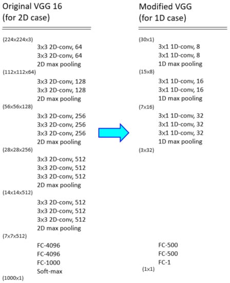
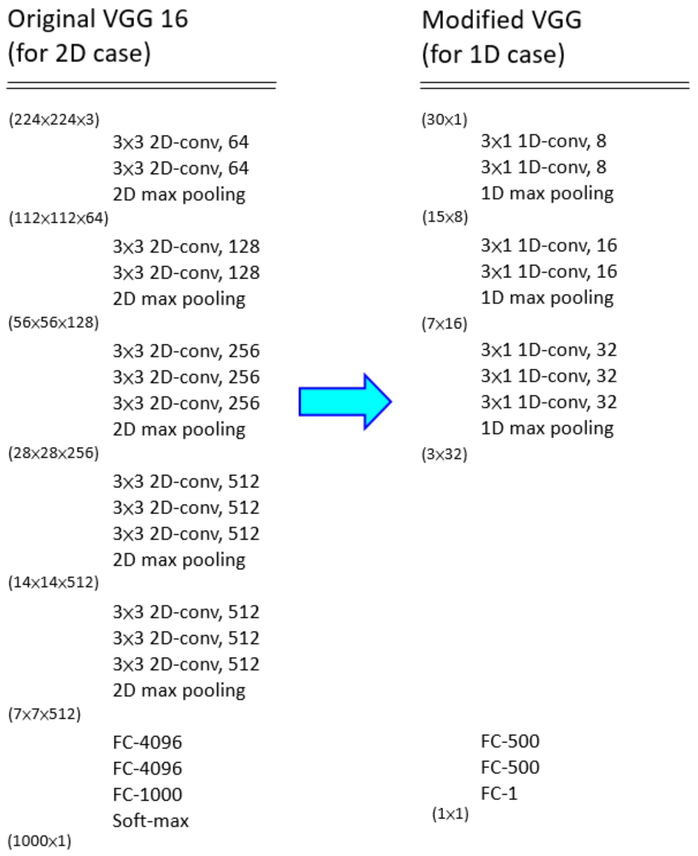
VGG is a popular CNN model containing 13 convolutional layers and three fully connected layers, commonly applied to image classification and pattern recognition. However, it is not directly suitable for building our surrogate model. In this paper, we instead use a simplified VGG model for this task. As the traditional VGG-16 model has a 2D layer structure consisting of many convolution layers, max-pooling layers, and fully connected layers, it is difficult to directly apply it to our steelmaking process-optimization problem with its 1D mapping. Therefore, we modified this VGG-16 model into a 1D structure with 10 layers (seven for 1D convolutional layers and three for fully connected layers). The seven convolutional layers generate powerful features, and three fully connected layers use the extracted features for regression.

More precisely, the differences between the traditional VGG-16 model and our simplified VGG model are shown in Figure 2. The simplified VGG model deletes the final soft-max procedure and maps the process parameters to a single product attribute. It is a one-dimensional CNN model composed of seven convolutional layers and three fully connected layers. The convolutional layers extract the powerful features, and the fully connected layers match the product attributes used when establishing the surrogate model. Our trained simplified VGG first uses three blocks in which two or three convolutional procedures are followed by max-pooling to obtain feature maps with sizes of 3×32; they are then straightened into one-dimensional form. The sequential fully connected layers are applied in order to regress the product attribute of $Y_1$, $Y_2$, or $Y_3$.

Figure 2. Traditional VGG and simplified VGG models.

In this method, the Adam algorithm [42] is used as an optimizer with a loss function equal to the mean square error (MSE) of the true outputs $\phi \left(x_l\right)$ of the surrogate model and the desired outputs $y_l$, as defined in Equation (21):

$$LossFunction=\frac{1}{M}{\displaystyle \sum }_{l=1}^M{\left(y_l-\phi \left(x_l\right)\right)}^2$$

(21)

3.3. Process Parameter Optimization Using the Firefly Algorithm

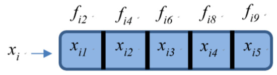
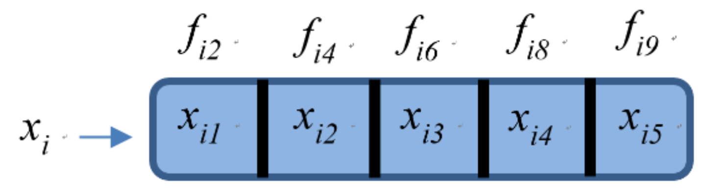
The process parameters of our test samples are divided into 25 fixed parameters and five adjustable ones, with the latter modified such that the product attributes meet the requirements. Therefore, we first assigned each adjustable process parameter to the i-th firefly solution $x_i$, with the structure depicted in Figure 3. Next, we used the FA to search for the optimal solution $x_{best.}$; first, we initialized N firefly solutions, $x_i, i=1,2,\dots ,N$, where each solution was updated using the FA.

Figure 3. Structure of firefly solution.

The fixed process parameters were integrated into each firefly solution $x_i$ into the $X_i$. Using the built surrogate model $\phi \left(X\right)$, the corresponding product quality attributes, Y_k = $\phi \left(X_i\right)$ for k = 1, 2, and 3, could be calculated. We then defined a fitness function as the brightness of the FA for the purposes of searching for the optimum, as shown in Equation (23).

$$u\left(X_i\right)=\frac{\left|Y_{i1}-m_{Y_1}\right|}{{\sigma }_{Y_1}}+\frac{\left|Y_{i2}-m_{Y_2}\right|}{{\sigma }_{Y_2}}+\frac{\left|Y_{i3}-m_{Y_3}\right|}{{\sigma }_{Y_3}}$$

(22)

$$Fitness\left(\mu \left(X_i\right)\right)=1/\left(1+u\left(X_i\right)\right)$$

(23)

where the product attributes $Y_{i1}$, $Y_{i2}$, and $Y_{i3}$ are the outputs of the surrogate model $\phi \left(x\right)$ with $x$ as its input, and $m_{Y_i}$ and ${\sigma }_{Y_i}$ are the mean and the standard derivation of the i-th product attributes of the training data samples.

The steps of the proposed algorithm are described in detail as follows:

Step 1.

Generate the initial solutions and the given hyper-parameters:

In this step, the initial population of N solutions is generated, as denoted by D = [$x_1,x_2,\dots .,x_N$], where $x_i=$ [f_i2, f_i4, f_i6, f_i8, f_i9] for the i-th firefly solution, and the values of $x_i$ are assigned from between −1 and 1. This step assigns the parameters of the FA, which are σ, ${\beta }_0$, the MCN, and γ. The number of cycles l is also set to 0.

Step 2.

Firefly movement:

Here, each complete process is combined into $X_i$, and its fitness value $Fitness\left(\mu \left(X_i\right)\right)$ is computed as the corresponding brightness of the firefly. For each firefly solution $x_i$, this step randomly chooses another brighter solution $x_j$ and then moves toward it, according to the following equations:

$$r_{ij}=||x_i-x_j||=\sqrt{{\displaystyle \sum }_{k=1}^5{(x_{ik}-x_{jk})}^{2 }}$$

(24)

$$x_{ik}=\left(1-\beta \right)x_{ik}+\beta x_{jk}+u_{jk}, \beta ={\beta }_0{e}^{-\gamma r_{i,j}}$$

(25)

where $u_{jk}~U\left(0,1\right)$ is a random number ranged from 0 to 1, and $x_{ik}$ is the k-th element of solution $x_i$.

Step 3.

Select the current best solution:

This step will pick the best solution from the solution set and represent it as $x_{best}$, as described by the following:

$$x_{best}=Argma{x}_{x_i}\left\{Fitness\left(\mu \left(x_i\right)\right)\right\}$$

(26)

Step 4.

Check the termination criterion:

If the cycle number l is equal to the MCN, the algorithm is finished and will output the best solution $x_{best}$. Otherwise, l increases by one and the best solution $x_{best}$ will randomly walk its position according to Equation (13). It will then return to Step 2 and repeat the process, as described by:

$$x_{best,k}=x_{best,k}+u_k, k=1, 2,\dots ,5$$

(27)

where $u_k$ is a random number ranged from 0 to 1.

Without a loss of generality, the PSO and ABC algorithms are also used to search for optimal parameters in a similar manner as the FA.

4. Results and Discussion

4.1. Training Mechanism by Using ML Methods

In experiments, the training parameters and strategy of the simplified VGG model are listed in Table 2, where each entry is optimal for the model. An initial learning rate of 0.001 and 250 training epochs were chosen in order to achieve adequate convergence. The Adam algorithm [25] was used as the optimizer and the mean square error as the loss function. A batch size of 50 was selected, and the average training time was 232.47 s.

Table 2. Parameters assigned in the simplified VGG model.

Method	Batch Size	Training Epochs	Trainable Variables	Initial Learning Rate	Loss Function	Optimizer	Average Training Time (s)
Simplified VGG Model	50	250	360,661	0.001	MSE	Adam	232.47

In order to evaluate the performance of a trained simplified VGG model, we computed the mean absolute error (MAE) (see Equation (28)) of the predicted and actual product attributes. The MAEs of $Y_1$, $Y_2$, and $Y_3$ are shown in Table 3, which reveals that the simplified VGG is the best, i.e., it is capable of producing strong correlations between the process parameters and the product attributes.

$$MA{E}_i=\frac{1}{299}{{\displaystyle \sum }}_{l=1}^{299}{\left|Y_{il}-\phi \left(X_l\right)\right|}^{}\hspace{0.33em}\hspace{0.33em}i=1,2,3$$

(28)

where $Y_{il}$ is i-th product attributes of l-th test sample.

Table 3. Mean absolute errors of the five surrogate model building methods.

	Linear Regression	Random Forests	Support Vector Regression	Multilayer Perception	Simplified VGG Network
Yield Stress, $Y_1$.	5.052 ± 0.09	3.890 ± 0.11	4.057 ± 0.09	4.156 ± 0.09	3.781 ± 0.08
Tensile Stress, $Y_2$	4.094 ± 0.10	3.647 ± 0.09	3.761 ± 0.10	3.798 ± 0.10	3.621 ± 0.08
Plastic Strain Ratio, $Y_3$	1.032 ± 0.02	0.954 ± 0.02	0.993 ± 0.02	0.948 ± 0.02	0.946 ± 0.02

(mean ± standard deviation).

4.2. Experimental Results of the Process Parameter Optimizations

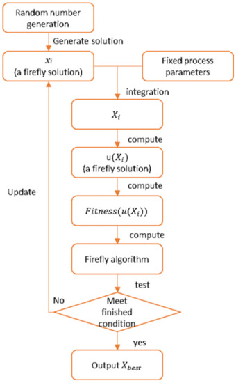
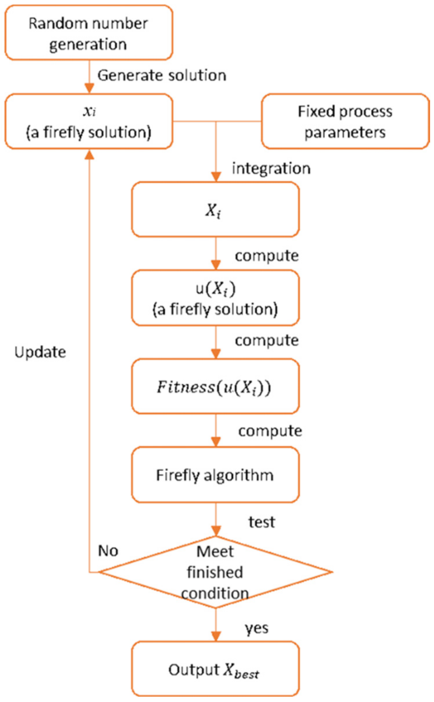
The FA was applied in order to search for the optimal adjustable process parameters of each of the test 299 samples, with the parameter settings of the algorithm given in Table 4. The FA is an iterative method, and a preassigned end condition is therefore needed. In this paper, we set the maximum number of iterations to 50 and the number of initial firefly solutions to 10. The average time spent searching for the optimal process parameters of each test sample was about 0.62 s. Additional details concerning the FA are shown in Figure 4.

Table 4. Parameter settings of the FA.

Parameter	Value
Attractiveness, ${\beta }_0$	1.0
Light Absorption Coefficient, γ	1.0
Number of Initial Firefly Solutions	10
MCL	50
σ	0.1

Figure 4. Flowchart of the FA used for optimizing the process parameters.

In our experiments, the 299 test samples were used to evaluate the performance of each method when searching for the optimal process parameters. The basis of evaluation is the success rate: how often the final product attributes fall in their reasonable quality ranges. Our experiments used the following combinations of methods: RF+PSO, RF+ABC, RF+Firefly, SVGG+PSO, SVGG+ABC, and SVGG+Firefly, the results of which are shown in Table 5. There we see that all the resulting test sample product attributes met their product quality requirements when the SVGG+Firefly combination was used, with its success rate of 100% clearly outperforming the other combinations.

Table 5. Success Rates of Different Combinations When Evaluating the 299 TestSsamples.

RF + PSO	RF + ABC	RF + Firefly	SVGG + PSO	SVGG + ABC	SVGG + Firefly
96.89%	97.99%	98.99%	97.32%	97.99%	100%

5. Conclusions

The optimization of process parameters is an important problem in steelmaking. In general, surrogate models can be applied to simulate the manufacturing process, although there are many different methods available to build such models. In this paper, we propose a simplified VGG model for this purpose and then compare it with other machine-learning methods. Within the model, different algorithms (PSO, ABC, and FA) were applied to obtain the optimal process parameters. In our experiments, we evaluated different combinations of trained surrogate models and searching methods. Our proposed simplified VGG model demonstrated to be the best method compared with the linear regression, random forests, support vector regression and multi-layer perceptron. The firefly algorithm is an effective search mechanism to optimize the process optimization in the simplified VGG surrogate model. It achieved a success rate of 100% in the 299 test samples, and these perfect results revealed that it has the potential to be effectively applied in different areas of process parameters optimization of product manufacture. Furthermore, it will be also an interesting thing how to develop a more complex and effective CNN model to build the surrogate model for other applications of process parameter optimization.

References

- Eric, M.; Stefanovic, M.; Djordjevic, A.; Stefanovic, N.; Misic, M.; Abadic, N.; Popović, P. Production process parameter optimization with a new model based on a genetic algorithm and ABC classification method. Adv. Mech. Eng. 2016, 8, 1–18. [Google Scholar] [CrossRef] [Scilit]
- Patil, V.D.; Sali, S.P. Process parameter optimization for computer numerical control turning on En36 alloy steel. In Proceedings of the 2017 International Conference on Nascent Technologies in Engineering (ICNTE), Navi Mumbai, India, 27–28 January 2017; pp. 1–5. [Google Scholar]
- Hoole, J.; Sartor, P.; Booker, J.D.; Cooper, J.E.; Gogouvitis, X.; Schmidt, R.K. Comparison of Surrogate Modeling Methods for Finite Element Analysis of Landing Gear Loads; Session: Surrogate Modeling for Uncertainty Quantification. In Proceedings of the AIAA Scitech 2020 Forum, Orlando, FL, USA, 6–10 January 2020. [Google Scholar]
- Salah, U.H.; Raman, P.S. Taguchi-based design of experiments in training POD-RBF surrogate model for in-verse material modelling using nanoindentation. Inverse Probl. Sci. Eng. 2017, 5, 363–381. [Google Scholar]
- Pfrommer, J.; Zimmerling, C.; Liu, J.; Kärger, L.; Henning, F.; Beyerer, J. Optimisation of manufacturing process parameters using deep neural networks as surrogate models. Procedia Cirp 2018, 72, 426–431. [Google Scholar] [CrossRef] [Scilit]
- Zhao, P.; Zhou, H.; Li, Y.; Li, D. Process parameters optimization of injection molding using a fast strip analysis as a surrogate model. Int. J. Adv. Manuf. Technol. 2010, 49, 949–959. [Google Scholar] [CrossRef] [Scilit]
- Forrester, A.I.; Keane, A.J. Recent advances in surrogate-based optimization. Prog. Aerosp. Sci. 2009, 45, 50–79. [Google Scholar] [CrossRef] [Scilit]
- Han, Z.-H.; Zhang, K.-S. Surrogate-Based Optimization. In Real-World Applications of Genetic Algorithms; IntechOpen: London, UK, 2012; pp. 343–362. [Google Scholar]
- Koziel, S.; Ciaurri, D.E.; Leifsson, L. Surrogate-Based Methods. In Computational Optimization, Methods and Algorithms; Springer: Berlin/Heidelberg, Germany, 2011; pp. 33–59. [Google Scholar]
- Simpson, T.; Poplinski, J.; Koch, P.N.; Allen, J. Metamodels for Computer-based Engineering Design: Survey and recommendations. Eng. Comput. 2001, 17, 129–150. [Google Scholar] [CrossRef] [Scilit]
- Cook, D.; Ragsdale, C.; Major, R. Combining a neural network with a genetic algorithm for process parameter optimization. Eng. Appl. Artif. Intell. 2000, 13, 391–396. [Google Scholar] [CrossRef] [Scilit]
- Thombansen, U.; Schuttler, J.; Auerbach, T.; Beckers, M.; Buchholz, G.; Eppelt, U.; Molitor, T. Model-based self-optimization for manufacturing systems. In Proceedings of the 2011 17th International Conference on Concurrent Enterprising, Aachen, Germany, 20–22 June 2011; pp. 1–9. [Google Scholar]
- Lovrić, M.; Meister, R.; Steck, T.; Fadljević, L.; Gerdenitsch, J.; Schuster, S.; Schiefermüller, L.; Lindstaedt, S.; Kern, R. Parasitic resistance as a predictor of faulty anodes in electro galvanizing: A comparison of machine learning, physical and hybrid models. Adv. Model. Simul. Eng. Sci. 2020, 7, 1–16. [Google Scholar] [CrossRef] [Scilit]
- Cemernek, D.; Cemernek, S.; Gursch, H.; Pandeshwar, A.; Leitner, T.; Berger, M.; Klösch, G.; Kern, R. Machine learning in continuous casting of steel: A state-of-the-art survey. J. Intell. Manuf. 2021. [Google Scholar] [CrossRef] [Scilit]
- Guo, S.; Yu, J.; Liu, X.; Wang, C.; Jiang, Q. A predicting model for properties of steel using the industrial big data based on machine learning. Comput. Mater. Sci. 2019, 160, 95–104. [Google Scholar] [CrossRef] [Scilit]
- Breiman, L. Random Forests. Mach. Learn. 2001, 45, 5–32. [Google Scholar] [CrossRef] [Scilit]
- Yan, C.; Yin, Z.; Shen, X.; Mi, D.; Guo, F.; Long, D. Surrogate-based optimization with improved support vector regression for non-circular vent hole on aero-engine turbine disk. Aerosp. Sci. Technol. 2020, 96, 105332. [Google Scholar] [CrossRef] [Scilit]
- Nauyen, T.H.; Nang, D.; Paustian, K. Surrogate-based multi-objective optimization of management options for agricultural landscapes using artificial neural networks. Ecol. Modeling 2019, 4, 1–13. [Google Scholar] [CrossRef] [Scilit]
- Jamshidi, M.B.; Lalbakhsh, A.; Alibeigi, N.; Soheyli, M.R.; Oryani, B.; Rabbani, N. Socialization of Industrial Robots: An Innovative Solution to improve Productivity. In Proceedings of the 2018 IEEE 9th Annual Information Technology, Electronics and Mobile Communication Conference (IEMCON), Vancouver, BC, Canada, 1–3 November 2018; pp. 832–837. [Google Scholar]
- Jamshidi, M.B.; Alibeigi, N.; Rabbani, N.; Oryani, B.; Lalbakhsh, A. Artificial Neural Networks: A Powerful Tool for Cognitive Science. In Proceedings of the 2018 IEEE 9th Annual Information Technology, Electronics and Mobile Communication Conference (IEMCON), Vancouver, BC, Canada, 1–3 November 2018; pp. 674–679. [Google Scholar]
- Jamshidi, M.B.; Lalbakhsh, A.; Talla, J.; Peroutka, Z.; Roshani, S.; Matousek, V.; Roshani, S.; Mirmozafari, M.; Malek, Z.; La Spada, L.; et al. Deep Learning Techniques and COVID-19 Drug Discovery: Fundamentals, State-of-the-Art and Future Directions. In Emerging Technologies during the Era of COVID-19 Pandemic; Springer: Berlin/Heidelberg, Germany, 2021; pp. 9–31. [Google Scholar]
- Xue, J.; Xiang, Z.; Ou, G. Predicting single freestanding transmission tower time history response during complex wind input through a convolutional neural network based surrogate model. Eng. Struct. 2021, 233, 111859. [Google Scholar] [CrossRef] [Scilit]
- Jia, X.J.; Liang, L.; Yang, Z.L.; Yu, M.Y. Muti-parameters optimization for electromagnetic acoustic transduces using surrogated-assisted particle swarm optimizer. Mech. Syst. Signal Process. 2021, 152, 107337. [Google Scholar] [CrossRef] [Scilit]
- Sun, L.; Sun, W.; Liang, X.; He, M.; Chen, H. A modified surrogate-assisted multi-swarm artificial bee colony for complex numerical optimization problems. Microprocess. Microsyst. 2020, 76, 103050. [Google Scholar] [CrossRef] [Scilit]
- Ewees, A.A.; Al-qaness, M.A.A.; Elaziz, M.A. Enhanced salp swarm algorithm based on firefly algorithm for unrelated parallel machine scheduling with set times. Appl. Math. Model. 2021, 94, 285–305. [Google Scholar] [CrossRef] [Scilit]
- Kiranyaz, S.; Avci, O.; Abdeljaber, O.; Ince, T.; Gabbouj, M.; Inman, D.J. 1D convolutional neural networks and applications: A survey. Mech. Syst. Signal Process. 2021, 151, 107398. [Google Scholar] [CrossRef] [Scilit]
- Simonyan, K.; Zisserman, A. Very deep convolutional networks for large-scale image recognition. arXiv 2014, arXiv:1409.1556. [Google Scholar]
- Zhang, M.; Long, D.; Qin, T.; Yang, J. A Chaotic Hybrid Butterfly Optimization Algorithm with Particle Swarm Optimization for High-Dimensional Optimization Problems. Symmetry 2020, 12, 1800. [Google Scholar] [CrossRef] [Scilit]
- Chao, C.-F.; Horng, M.-H.; Chen, Y.-C. Motion Estimation Using the Firefly Algorithm in Ultrasonic Image Sequence of Soft Tissue. Comput. Math. Methods Med. 2015, 343217. [Google Scholar] [CrossRef] [Scilit] [PubMed]
- Liu, W.; Huang, Y.; Ye, Z.; Cai, W.; Yang, S.; Cheng, X.; Frank, I. Renyi’s Entropy Based Mutlilevel Thresholding Using a Novel Meta-Heuristic Algorithm. Appl. Sci. 2020, 10(9), 3225. [Google Scholar] [CrossRef] [Scilit]
- Horng, M.H. Multilevel thresholding selection based on the artificial bee colony algorithm for image segmentation. Expert Syst. Appl. 2011, 38, 13785–13791. [Google Scholar] [CrossRef] [Scilit]
- Kaminski, M. Neural Network Training Using Particle Swarm Optimization—A Case Study. In Proceedings of the 2019 24th International Conference on Methods and Models in Automation and Robotics (MMAR), Miedzyzdroje, Poland, 26–29 August 2019; pp. 115–120. [Google Scholar]
- Lalbakhsh, A.; Afzal, M.U.; Esselle, K.P. Multi-objective Particle Swarm Optimization to Design a Time-Delay Equalizer Metasurface for an Electromagnetic Band-Gap Resonator Antenna. IEEE Antennas Wirel. Propag. Lett. 2016, 16, 912–915. [Google Scholar] [CrossRef] [Scilit]
- Lalbkhsh, A.; Esselle, K.P. Directivity Improvement of a Fabry-Perot Cavity Antenna by enhancing Near Field Characteristic. In Proceedings of the 17th International Symposium on Antenna Technology and Applied Electromagnetics, Montreal, QC, Canada, 10–13 July 2016. [Google Scholar]
- Lalbakhsh, A.; Afzal, M.U.; Esselle, K. Simulation-driven particle swarm optimization of spatial phase shifters. In Proceedings of the 2016 International Conference on Electromagnetics in Advanced Applications (ICEAA), Cairns, QLD, Australia, 19–23 September 2016; pp. 428–430. [Google Scholar]
- Kennedy, J.; Eberhart, R. Particle swarm optimization. In Proceedings of the ICNN’95—International Conference on Neural Networks, Perth, WA, Australia, 27 November–1 December 1995; Volume 6, pp. 1942–1948. [Google Scholar]
- Karaboga, D.; Basturk, B. On the performance of artificial bee colony (ABC) algorithm. Appl. Soft Comput. 2008, 8, 687–697. [Google Scholar] [CrossRef] [Scilit]
- Łukasik, S.; Żak, S. Firefly Algorithm for Continuous Constrained Optimization Tasks. In International Conference on Computational Collective Intelligence; Springer: Berlin/Heidelberg, Germany, 2009; pp. 97–106. [Google Scholar]
- Yang, X.-S. Firefly Algorithms for Multimodal Optimization. In International Symposium on Stochastic Algorithms; Springer: Berlin/Heidelberg, Germany, 2009; pp. 169–178. [Google Scholar]
- Yang, X.S. Nature-Inspired Metaheuristic Algorithms; Luniver Press: Frome, UK, 2008. [Google Scholar]
- Lalbakhsh, P.; Zaeri, B.; Lalbakhsh, A. An Improved Model of Ant Colony Optimization Using a Novel Pheromone Update Strategy. IEICE Trans. Inform. Syst. 2013, E96-D, 2309–2318. [Google Scholar] [CrossRef] [Scilit]
- Kingma, D.P.; Ba, J. Adam: A method for stochastic optimization. arXiv 2014, arXiv:1412.6980. [Google Scholar]
Publisher’s Note: MDPI stays neutral with regard to jurisdictional claims in published maps and institutional affiliations. |
© 2021 by the authors. Licensee MDPI, Basel, Switzerland. This article is an open access article distributed under the terms and conditions of the Creative Commons Attribution (CC BY) license (https://creativecommons.org/licenses/by/4.0/).