Article

Discovering Intra-Urban Population Movement Pattern Using Taxis’ Origin and Destination Data and Modeling the Parameters Affecting Population Distribution

by
Fatema Rahimi
1,†,
Abolghasem Sadeghi-Niaraki
1,2,†,
Mostafa Ghodousi
1 and
Soo-Mi Choi
2,*
1
Geoinformation Technology Center of Excellence, Faculty of Geodesy and Geomatics Engineering, K.N. Toosi University of Technology, Tehran 19697, Iran
2
Department of Computer Science and Engineering, and Convergence Engineering for Intelligent Drone, Sejong University, Seoul 143-747, Korea
*
Author to whom correspondence should be addressed.
These authors contributed equally to this work.
Appl. Sci. 2021, 11(13), 5987; https://doi.org/10.3390/app11135987
Submission received: 25 April 2021 / Revised: 7 June 2021 / Accepted: 9 June 2021 / Published: 27 June 2021

Abstract

:
GPS-equipped vehicles are an effective approach for acquiring urban population movement patterns. Attempts have been made in the present study in order to identify the population displacement pattern of the study region using taxis’ origin and destination data, and then model the parameters affecting the population displacement pattern and provide an ultimate model in order to predict pick-up and drop-off locations. In this way, the passenger pick-up and drop-off locations have been identified in order to obtain the population movement pattern. In this study, Moran’s I index was used to measure the spatial autocorrelation, and hot spot analysis was used to analyze spatial patterns of pick-up and drop-off locations. Effective parameters modeling was performed using the Poisson regression. The results of the spatiotemporal distribution map for pick-up and drop-off locations indicated a similarity in patterns and equal results for some locations. Results also indicated different features of spatial distribution during different hours of the day. Spatial autocorrelation analysis results indicated a low probability of randomness in the general spatial distribution of the locations. The result of modeling the parameters shows the positive effect of the parameters on the pattern of population movement, and according to the p-value of 0.000, Poisson regression is significant for the pick-up and drop-off locations. The modeling results also highlighted the importance of movement patterns in recognizing urban hot spots, which is valuable for policymakers and urban planners.

1. Introduction

With the rapid growth of the city, urban planners face many challenges. The unplanned development of cities and populations has imposed many problems on planners at various levels. Understanding urban growth and its related factors and their impact on the city should be considered by urban planners. Urban growth is directly related to transportation and, consequently, urban traffic. Part of urban planning is a transportation planning and urban traffic [1,2]. Lack of attention to urban planning and transportation planning leads to a lack of sustainable development [3]. Urban planning and its context are also continuous, permanent, and dynamic and cannot be dealt with in a cross-sectional, temporary, and static manner. On the other hand, understanding the pattern of transport requires understanding the movement behavior of individuals [4]. Therefore, there is a need to study the spatiotemporal growth of the urban environment and the movement behavior of individuals to achieve sustainable urban development. In an urban environment, an important part of human activity is the movement behavior of individuals, and a thorough analysis can lead to the extraction of a movement pattern. With the rapid advancement in IT and communication technologies, research about human movement in recent years has risen [5]. The discovery of movement patterns helps recognize the spatial and temporal structure of cities [6]. Understanding urban populations’ movement and temporal patterns are useful in areas such as urban planning, urban management, and urban traffic modeling and forecasting [7]. Additionally, given the prevalence of the coronavirus, spatiotemporal population modeling can be used to predict epidemics. A population with a high rate of displacement can spread the disease more rapidly. In areas with high population movements, the spread of the disease is higher because the arrivals and departures are high, and residents have to travel longer distances to do their jobs [8].
We live in a data-rich world where analyzing this big data can solve many of our problems [9]. Therefore, big data of intra-city travel can be useful in many spatial analysis. These studies have great importance in various applications such as traffic control, land use planning, and other applications [10,11], especially in the densely populated and developing cities of Iran, which face a variety of problems. One of these developing cities facing a high growth rate is Bojnourd, the capital of the Northern Khorasan province. Few studies in Iran have explored the patterns of population movement, which necessitates this research. In addition, in past studies, less attention has been paid to predict pick-up and drop-off locations based on the parameters affecting the movement pattern. Therefore, this research has explored the movement patterns of Bojnourd’s inhabitants, using taxis’ origin and destination data.
This paper initially identifies the movement patterns by data pre-processing and then segmenting the studied area into smaller pieces; Moran’s I will be applied to evaluate spatial autocorrelation, and hot spot analysis will be used to investigate the spatial patterns of pick-up and drop-off locations. Then, the process of modeling the parameters influencing the population movement patterns continues to further predict taxis’ pick-up and drop-off locations distribution.
This study begins with a brief introduction justifying the necessity of the research, its implementation, and then the scope of the study areas. The following parts present the research methodology, findings, discussion, and conclusion.

2. Relevant Literature

Urban trip distribution estimation methods are divided into three categories: field survey methods (the traditional approach), counting sensor methods, and methods based on location-oriented technologies [12,13]. Though temporal and spatial patterns could be explored using the traditional method, such data sets are not always enough to measure microscopic travel behavior [14]. In the counting sensor method, urban traffic rates are estimated by sensors and traffic cameras, which are limited options due to high installation and maintenance costs [15]. In general, these models tend to have computational complexity. Methods relying on location-oriented technologies include mobile data, social networking inputs, Bluetooth tracking data, and locations registered by the Global Positioning System (GPS) system [16,17,18].
Data types related to the third category have been used in various studies. Some studies have used mobile phone data to discover the general spatial pattern of the population [19]. Gariazzo et al. [20] used mobile data and demographic data to explore the spatiotemporal pattern of population in Rome. Using large mobile data, Yang et al. [21] and Wu et al. [22] examined the spatiotemporal pattern of population movement in China. However, the problem with this type of study is that people do not desire to share their location because of their privacy [23]. In recent years, intelligent transportation systems have been including GPS-equipped taxis to alert and enhance transportation management. The route data, including location and speed, sent by moving vehicles are stored in a data center. Utilizing real-time data systems to manage traffic make it possible to monitor urban traffic and make predictions about probable congestions [24]. The data acquired from GPS-equipped taxis have been utilized in a few cases in current studies with geographical purposes.
In the past few years, taxi GPS data have been studied as a suitable way to explore the patterns of movement of people in different studies [25,26]. Yuan and Le Noc [27] examined the urban movement using taxi-induced data in the Chinese city of Nanjing, which clearly distinguished between city centers and suburbs. Gong et al. [28] speculated the purpose of traveling and identified the traveling patterns from the taxis trajectory data in Shanghai. The study approximates the Shanghai residents’ journey. Shen et al. [29] proposed a method to draw out passenger pick-up and drop-off locations, discovering the spatial movement pattern of the Nanjing population using taxi data. Rahimi et al. [30] have spatially-temporally modeled the population of Bojnourd using data from the origin and destination of taxis and discovered the movement pattern of the population. The results of the study showed that the method used to model the population at the neighborhood level worked well. Some studies have also examined the movement pattern during the coronavirus pandemic. La Gatta et al. [8] predict the spread of an epidemic using a framework based on machine learning and movement data and the spatiotemporal effects of an epidemiological model. The comparison of trained epidemic models with actual data showed the good performance of the model. In general, it can be acknowledged that in most of the researches, the movement pattern of people has been identified using taxi position data, and the parameters affecting the movement pattern of people have been paid less attention to predict the pick-up and drop-off locations.
Recently, several methods have been developed to study the patterns of city movement by using taxi origin and destination data. Spatial data clustering is one of the most largely used methods, which is generally used for a group of similar objects. Exploratory analysis is a suitable method for displaying and describing spatial distributions, discovering spatial relationship patterns, and identifying spatial clusters. These methods show local and global spatial autocorrelation and spatial heterogeneity [31]. The spatial autocorrelation method may be used to measure the spatial interaction of numeric interval and ratio data [32]. In addition, spatial autocorrelation methods have been used in some studies. Saddam Hussain et al. [33] examined the spatial pattern of vehicle accidents by spatial autocorrelation. Moran’s I statistic cannot detect spatial clusters that are presented as hot spots and cold spots. Therefore, local statistics G was used. The Getis-Ord-Gi statistic is a remarkably useful method in evaluating the local autocorrelation of space. This method detects areas with greater contribution to spatial autocorrelation to identify local clusters with high or low values. Besides, these methods also identify specific sections or adjacent section groups that deviated from their general spatial autocorrelation.
Various factors such as land use, the regional population, area, etc., impact the population movement patterns. Identifying and recognizing such factors and determining the scope of their influence makes it possible to control the population growth and specific uses through appropriate necessary planning. Depending on the dependent variable’s type, different modeling methods are implementable; when the target and response variable’s data are numeric and discrete, the efficiency of multiple linear regression models, Poisson, and negative binomials is so remarkable. Logistic models indicate acceptable and near-realistic results [34]. When the dependent variable’s data are categorical (occurrences and non-occurrences). The Poisson regression model is utilized in a wide range of data sets. Often, this method is a good starting point model as long as the data is distributed by Poisson. Poisson distribution is used wherever counting data are considered [35]. According to the type of data related to pick-up and drop-off locations, which are of the numerical type and the number of these points in various places is independent of each other, the modeling of parameters affecting the population movement pattern will be carried out using the Poisson model in this study.

3. The Study Area

Bojnourd is the capital of the Northern Khorasan province in northeastern Iran. Bojnourd, with 36 square kilometers, is at 57°20′ longitude and 37°28′ latitude in the foothills of Aladagh, Kopeh Dagh, and Alborz Mountains. One of the largest cities in the country, Bojnourd is ranked the forty-fourth city in Iran. Based on the latest population and housing census of 2016, the population is 228,931 (67,335 households). In the last decade, with the creation of the Northern Khorasan and being chosen as the center of this new province and extensive migration, Bojnourd has been facing rapid population growth and a rapid extension of the state. Traffic is a problem the majority of growing cities are dealing with. A large number of citizens traverse Bojnourd, the capital of the Northern Khorasan, in the scope of a day, hence the importance of traffic for urban planners, which contributed to the conduction of this study. The study area is shown in Figure 1.

4. Data and Research Method

The present study is a descriptive-analytical method aimed at identifying the pattern of intra-urban population movement using taxis’ origin and destination data and modeling the parameters that affect the population movement pattern in Bojnourd. In this research, taxis’ GPS data in Bojnourd were exploited to compute the number of trips produced and evaluate the models. Taxi data were collected from 137 taxis from 1 November 2018 to 26 December 2018. The format of the raw taxi data was the trajectory of taxis, including 20,008,969 data, with each record containing information concerning taxi identification, position, speed, direction, time, cost, and whether or not the passenger is carrying (status). Table 1 provides a sample record of the data set. Other data included land use (residential areas, workplaces, educational facilities, kindergartens, clinics, hospitals, etc.) and population (population size).
This study initially identified the intra-urban populationn movement and the accuracy of the model in predicting the number of pick-up and drop-off points was examined. The first step to identifying population movement patterns was data preprocessing, drawing out pick-up and drop-off locations, and detecting and removing trips outside the study area. Finally, the number of trips produced and absorbed in each region was calculated. In the end, Moranp and drop-off loplied to evaluate spatial autocorrelation, and Getis-Ord-Gi hot spot analysis was applied to analyze spatial patterns of pick-up and drop-off locations. Poisson regression was utilized to model the parameters impacting the population movement, and the accuracy of the model in predicting the number of pick-up and drop-off points was examined. Figure 2 describes the stages of research.

4.1. Identify the Pattern of Intra-Urban Population Movement Using Taxis’ Origin and Destination Data

The first step toward identifying population movement patterns was to preprocess the data and extract passenger pick-up and drop-off locations. The pick-up and drop-off locations were obtainable when the passenger’s status changes. When the passenger’s previous status was set to 0 and the current passenger status was set to 1, the sample point represented a pick-up location. If the passenger’s previous status was 1 and the passenger’s current status was 0, it was assumed that the current sample point is a drop-off location [36,37]. A total of 112,050 pick-up locations and 105,256 drop-off locations were extracted. Points that originated outside the study area or were terminated outside the study area were identified and then removed. A total of 12,204 pick-up locations and 18,258 drop-off locations were excluded, and finally, 99,846 pick-up locations and 86,998 drop-off locations were retained. Excluding pick-up and drop-off locations comprised only 10.9% and 17.3% of the total pick-up and drop-off locations. Finally, the regional number of pick-up and drop-off locations was calculated. Figure 3 depicts the spatial distribution of pick-up and drop-off locations in the research area.
First, before the data analysis step, it was necessary to assign pick-up and drop-off locations to the study area. After data preparation, Moran’ I statistic was used for analyzing the spatiotemporal pattern of the urban population movement. In spatial statistics, recognizing patterns and discovering the trend in spatial data have particular importance. Moran’s I spatial autocorrelation statistic makes it possible to measure spatial differences among all samples. To calculate Moran’s I index, first, a score of Z and a p-value must be obtained, and then the evaluation and significance of Moran statistic should be considered. The value of Moran’s I varies between −1 and 1. Negative Moran values indicate a negative trend in spatial autocorrelation and positive values indicate a positive trend in the autocorrelation of space, and the zero value represents a random spatial pattern [38] The value of the Global Moran’s I is calculated by Equation (1) [39].
I = n s 0 × i = 1 n j = 1 n w i j x i x ¯ x j x ¯ i = 1 n   x i x ¯ 2
If n represents spatial units number specified with i and j; then X is the desired variable; X ¯ is the mean of X; Wij is a part of the spatial weights matrix and the number of points in a study unit. S0 also indicates the sum of all the elements. In general, spatial autocorrelations depend on Z values. Spatial clustering is a high value if the Z score is both positive and high. However, if the Z score is negative and low, spatial clustering is of low value. Additionally, when Z score is statistically significant, its values are larger than the expected values of 1.96 or more than 2.58 [40]. The z-score can be shown mathematically as Equation (2) [41,42].
E I = 1 n 1   a n d   V I = E I 2 E I 2   z = 1 E I V I
The value of p represents a probability. If this value is very small, there is a low probability of the spatial pattern observed being the outcome of accidental processes; then, the null hypothesis can be rejected. If the yielded value of p is less than 0.01, it indicates a probability of 1% of this clustered pattern being the product of a random process [40].
It is also necessary to use local spatial autocorrelation to determine the location of hot spots and cold spots. The statistic of Getis-Ord-Gi was used to explore more precisely the spatial distribution of hot spots and cold spots. When this statistic is obtained, the confidence level is considered to be 90%, 95%, and 99%, respectively. The Getis-Ord-Gi statistic is calculated as Equation (3) [43].
G i * = j = 1 n w i , j x j x ¯ j = 1 n w i , j s n j = 1 n w i j 2 j = 1 n w i j 2 n 1               x ¯ = j = 1 n x j n       a n d       s = j = 1 n x j 2 n x ¯ 2      
where xj is the attribute value for the attribute J; wi,j is the spatial weight between the property i and j; n is the total number of attributes.

4.2. Modeling the Parameters Affecting Population Distribution

In order to model the parameters affecting population movement, first, the identification of effective parameters, such as pick-up and drop-off locations, area, number of types of land use, number of migrations, and the population of the region, was performed. Then, modeling was conducted using Poisson regression. One of the most important general linear models is the Poisson model, which uses the Poisson distribution for the response variable and assumes that the mean and variance of the response variable are equal [35]. In a Poisson model, the probability of the ith neighborhood, which has yi pick-up and drop-off locations, is obtained by Equation (4). The relationship between the independent variables and the number of pick-up and drop-off locations for the expected study area is a logarithmic, linear model derived from Equation (5). The general form of the model is depicted in Equation (6) [44].
P y i = exp λ i λ i y i y i !
l n λ i   =   β X i                   o r                 λ i   =   exp β X i
λ i = e β 0 + β 1 x 1 + β 2 x 2 + + β n x n
P(yi) is the probability of ith neighborhood of the study area which has yi pick-up and drop-off locations. yi shows the number of pick-up and drop-off locations for ith neighborhood. β is a regression parameters vector and Xi is an independent variables vector. β0 is the constant coefficient, β1, ... and βn are the calculated coefficients in the vector form and x1, ... and xn are independent variables. Finally, the model is validated to predict the number of pick-up and drop-off points to determine its efficiency and adequacy in modeling the number of pick-up and drop-off points.

5. Results

The results and discussion section begin with depicting of the spatiotemporal pattern of population movement in Bojnuord, using the inter-urban taxis’ origin and destination data. The findings related to identifying the factors impacting the population movement patterns were then presented.

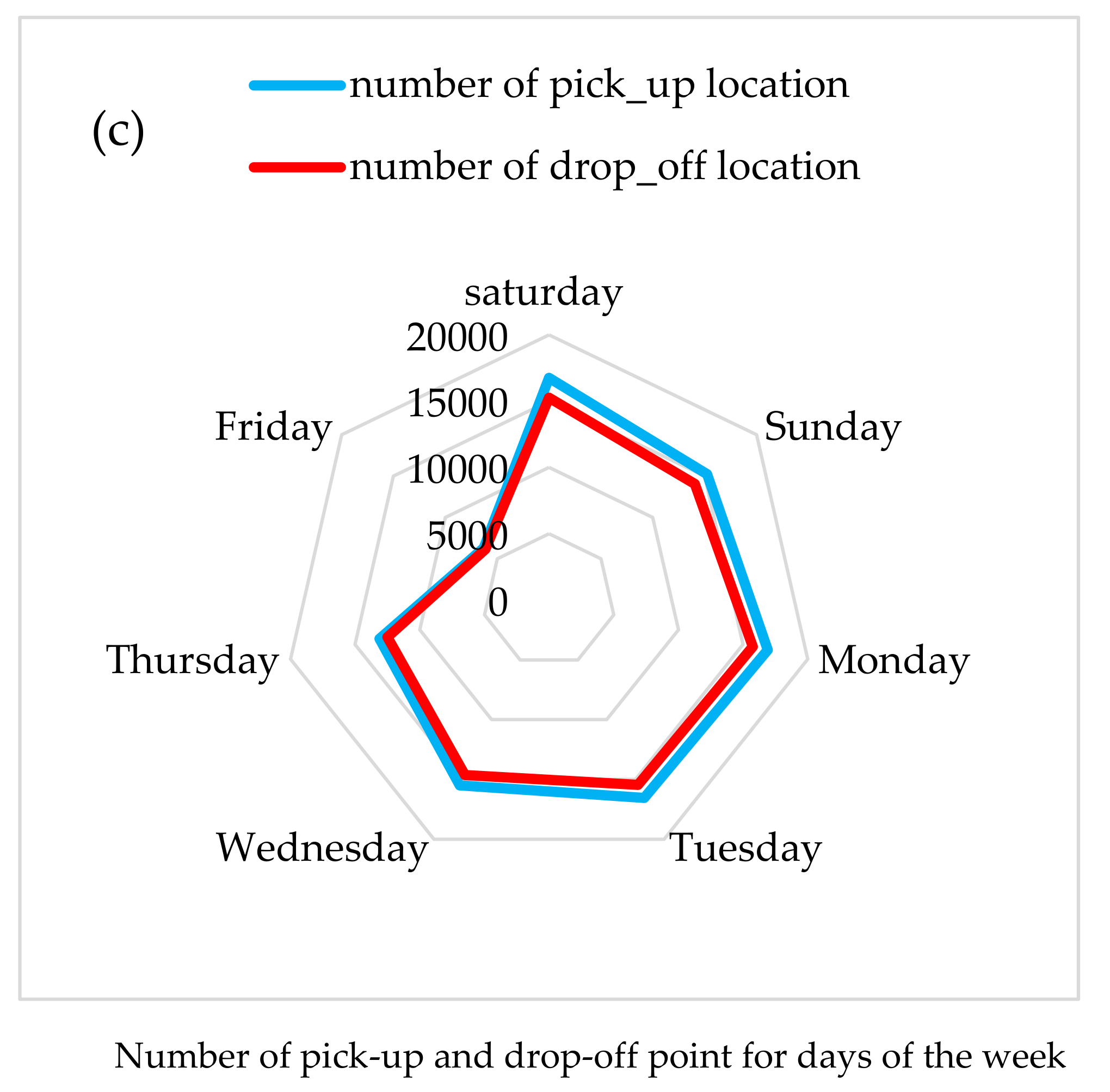
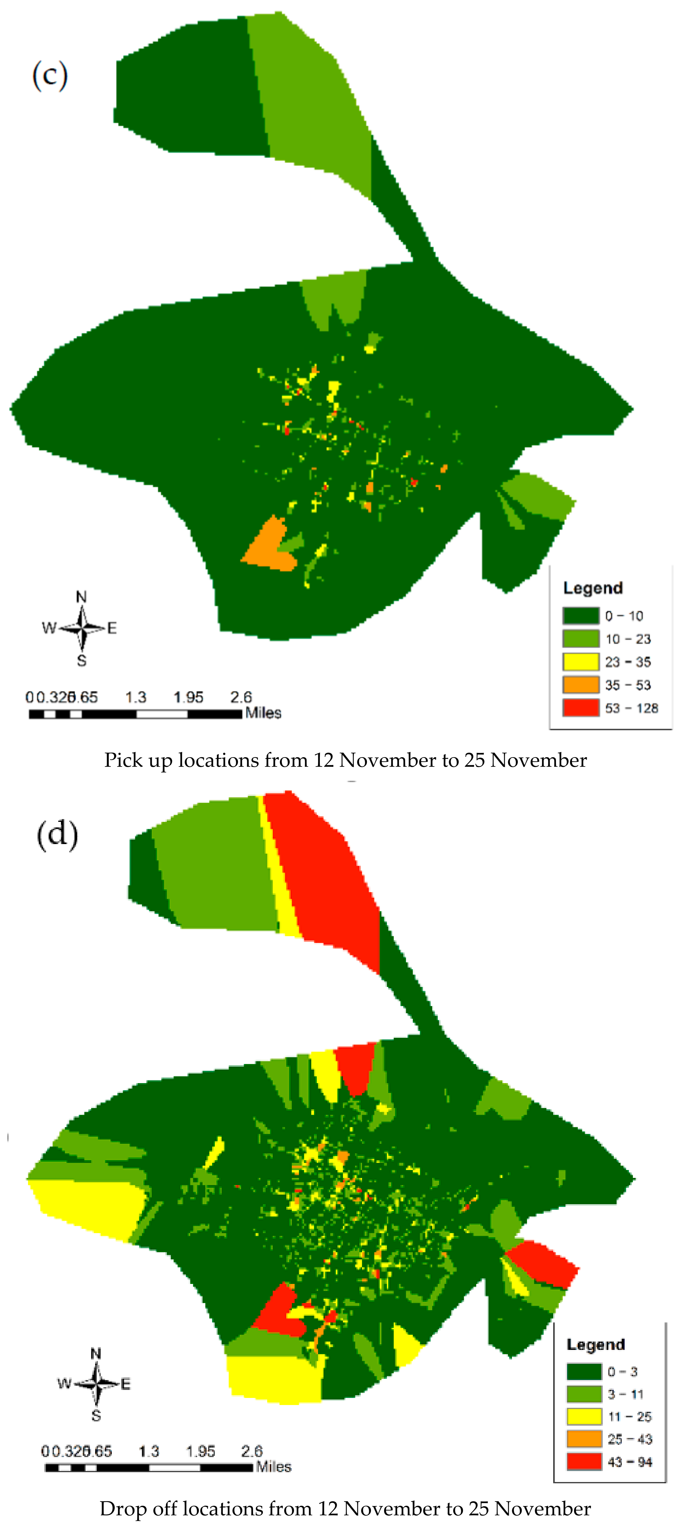
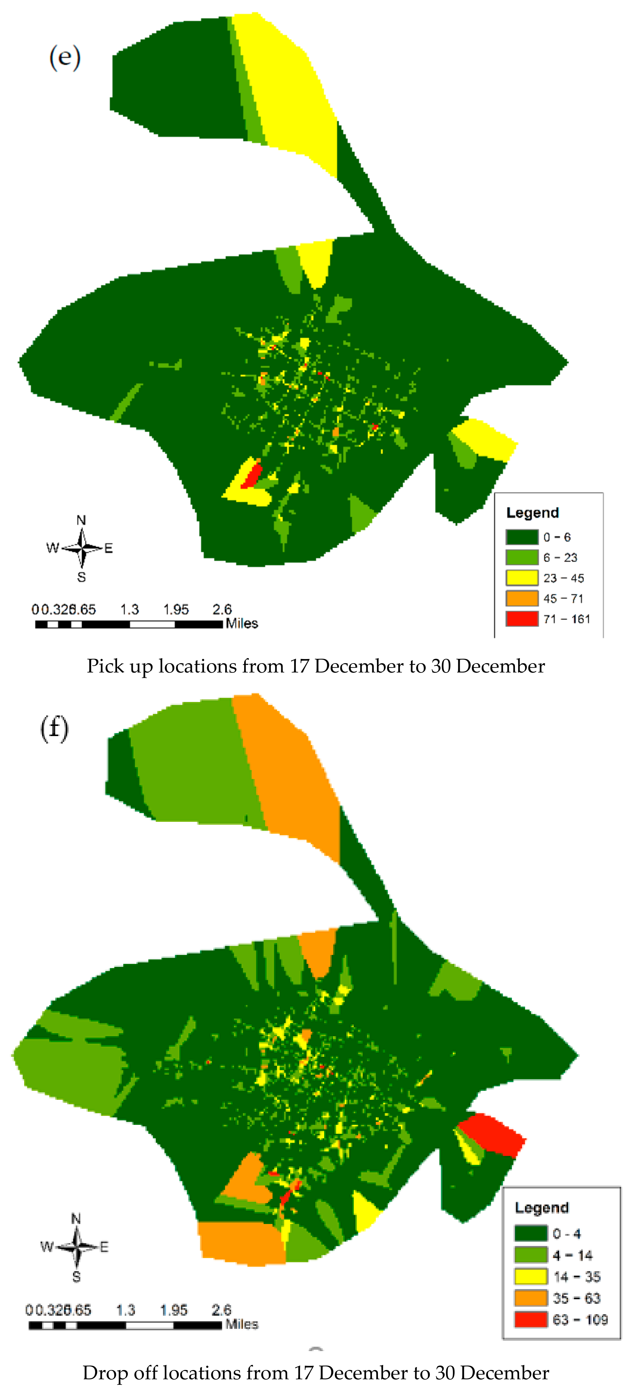
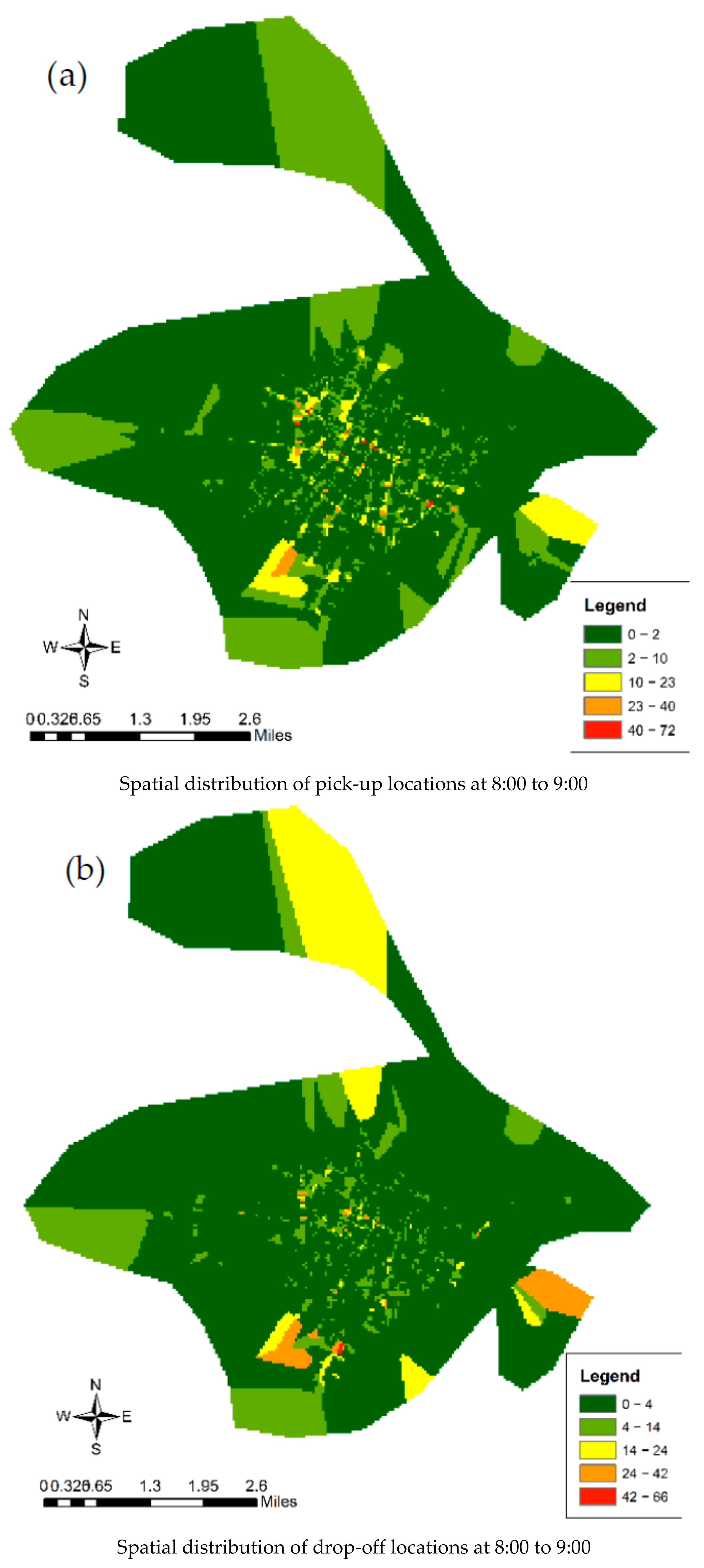
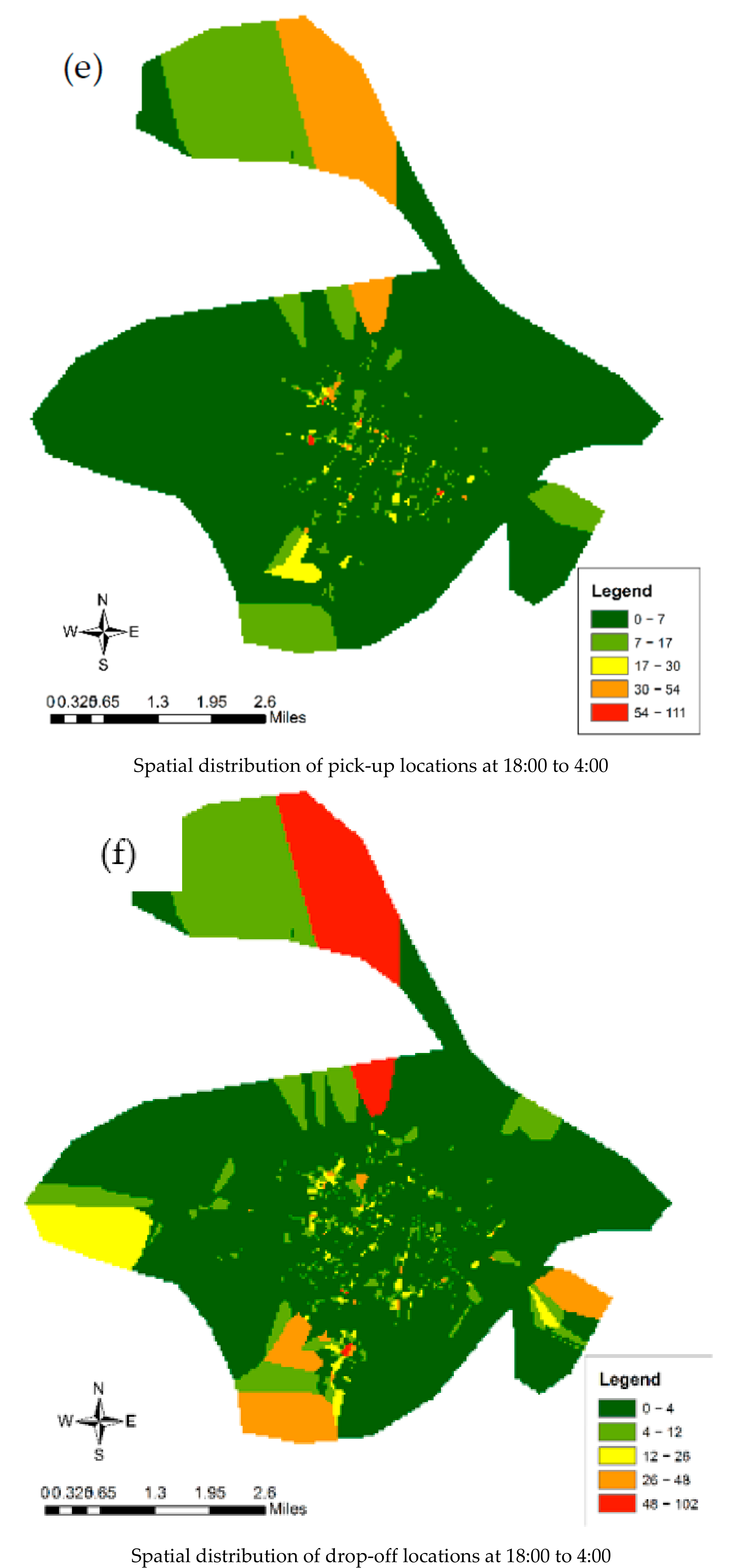
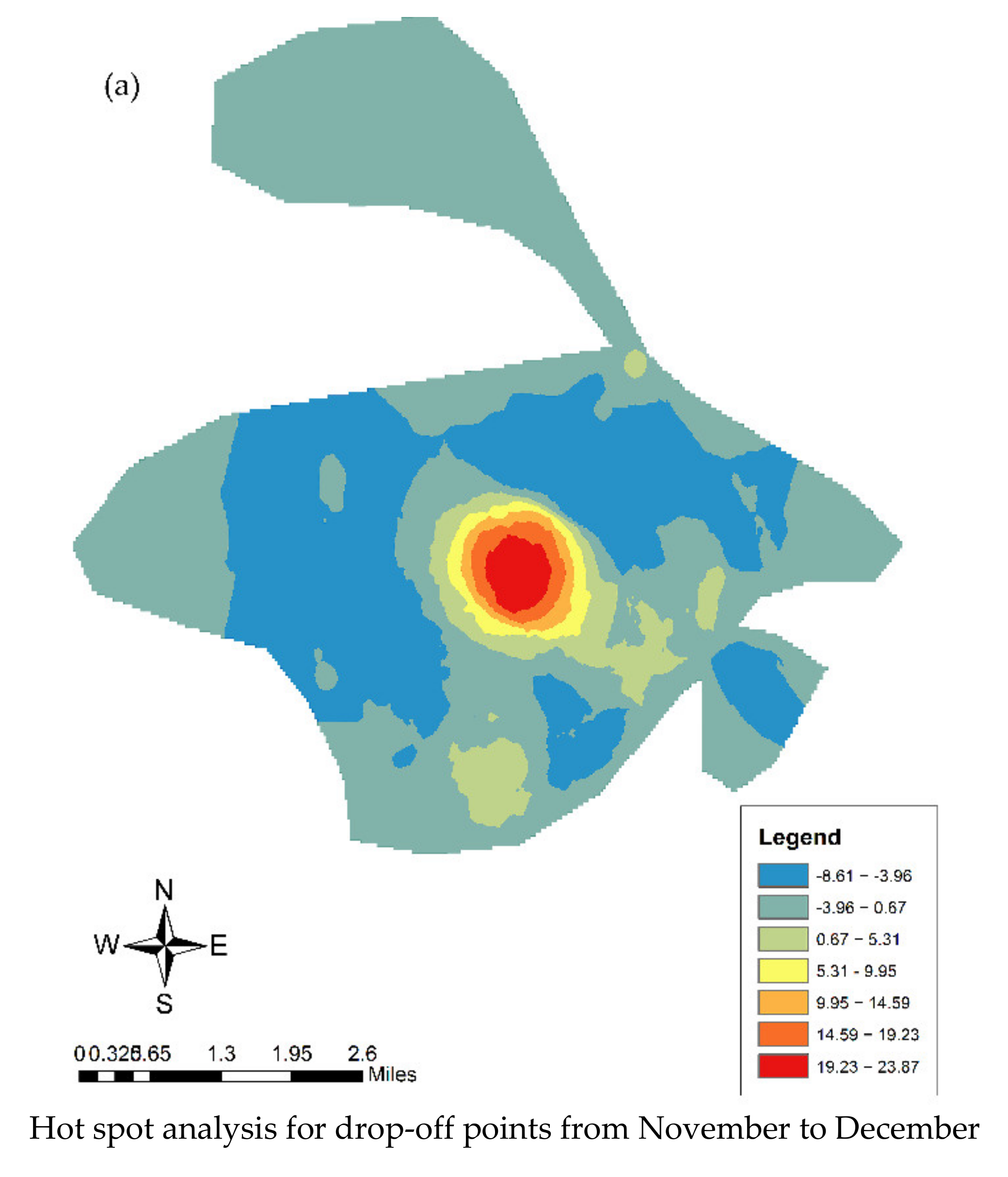
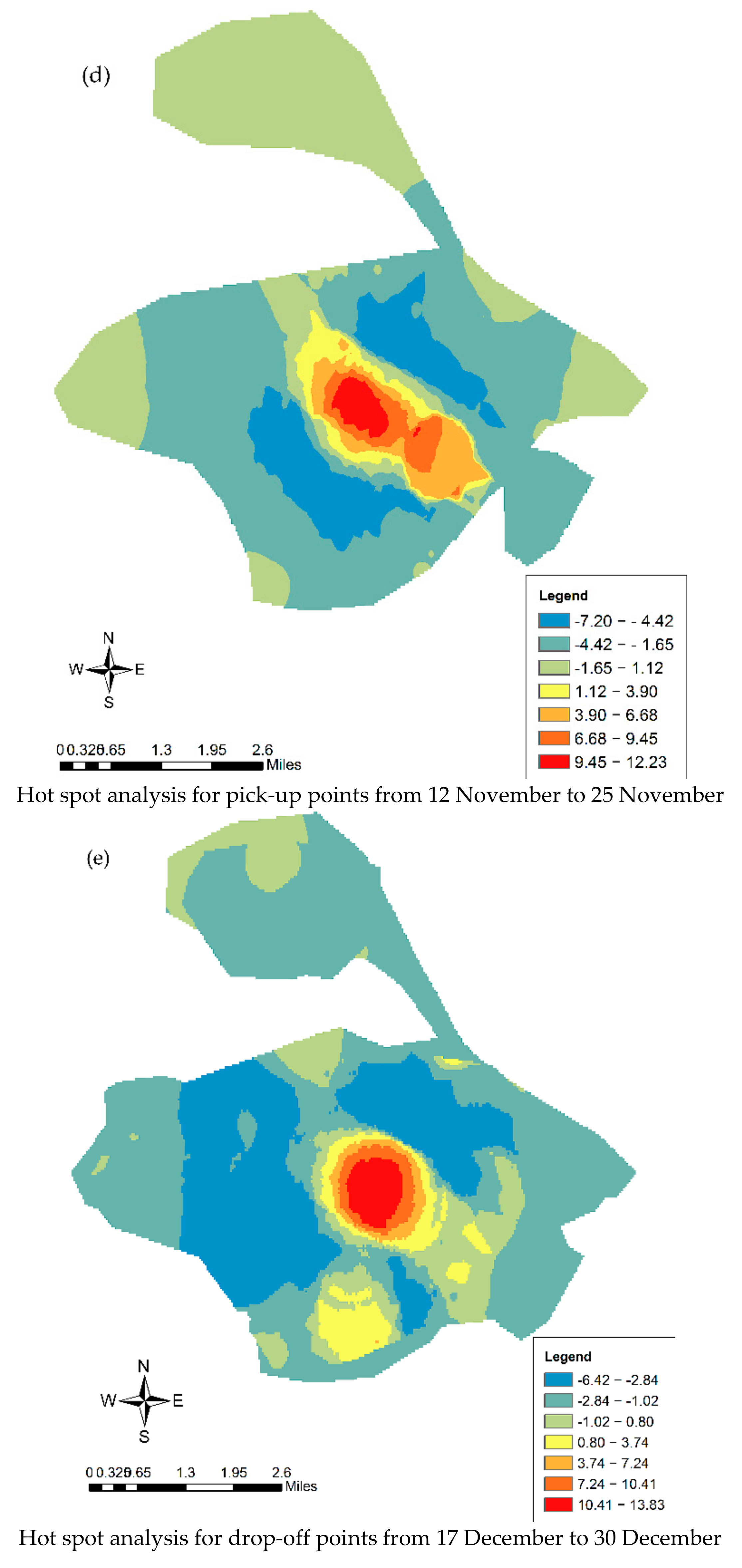
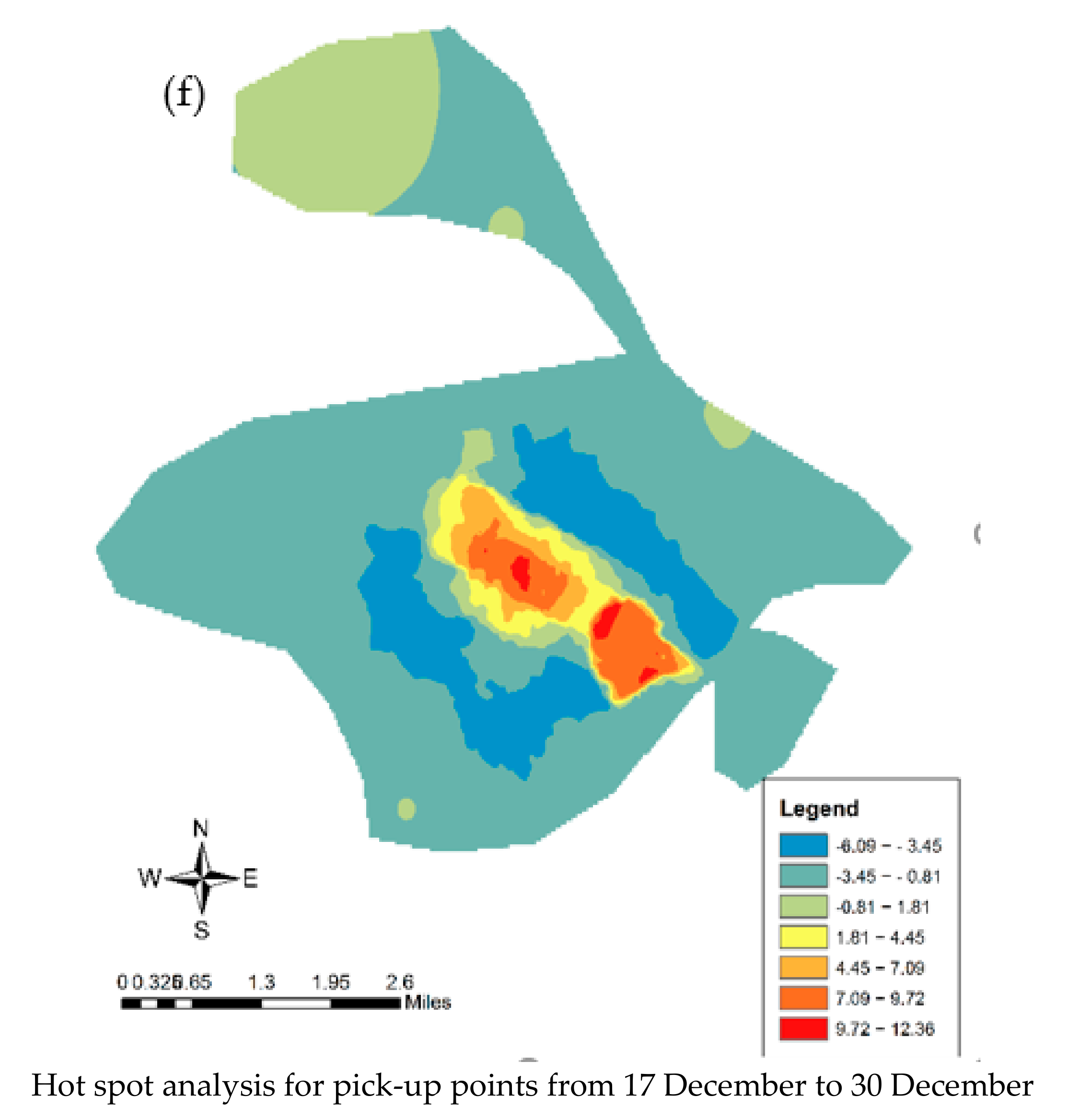
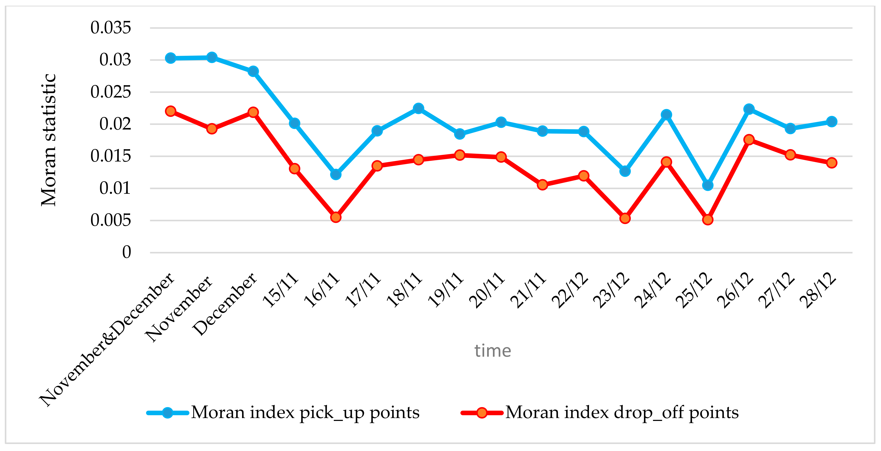
5.1. Spatiotemporal Pattern of Population Movement

In this research, GPS data of taxis in the urban areas of Bojnuord were used to identify the behavioral pattern of urban movement. After processing the data, the pick-up and drop-off locations statistics within one-hour scales were obtained daily and on the weekdays. Figure 4 represents the number of pick-up and drop-off locations per hour, per day in a week.
On a daily scale, a similar pattern and an almost equal number of pick-up and drop-off locations per day are examined. On a weekly scale, Fridays and Thursdays depict lower numbers than the rest of the days of the week. Expectedly, statistics indicate taxi travels are lower at weekends and that a similar pattern is examinable across all weekdays. On an hourly scale, results depict different spatial distribution patterns at different hours per day. With the working hour beginning in the morning, the rush hour rises from 8:00 to 9:00. Besides, from 14:00 to 15:00, when the daily work is completed and the passengers return to their homes, another rush period is expected. There is also a reduction in the congestion period from 18:00 to 4:00. There are plenty of pick-up and drop-off locations available from 4:00 to 18:00.
Figure 5 depicts the distribution of pick-up and drop-off locations in November and December, and Figure 6 depicts the spatial and temporal distribution from 8:00 to 9:00, 14:00 to 15:00, and from 18:00 to 4:00.
November and December represent a similar spatial pattern of the pick-up and drop-off locations spatial distribution. Expectedly, the majority of daily trips begin from downtown. As depicted in Figure 5, there is a clear division between the suburbs and the urban center, where taxi trips tend to be carried out toward far locations of the urban center or toward a specific center, indicating there is a clear separation of crowded urban areas in which residents can take a short trip for their daily needs in any center or suburbs. Movement activities occur during the day and often gradually resume from morning until night. As shown in Figure 6, the pick-up and drop-off locations’ number varies over time. Additionally, the number of pick-up and drop-off locations during the day is more than the night (8:00–9:00), due to travel to the workplace, and 14:00–15:00, because of returning from work.
The map consisting of the pick-up and drop-off locations, hot and cold spots, is demonstrated in Figure 7. Getis-Ord-Gi statistic identifies hot spots with accuracy levels up to 90, 95, and 99 percent. Hot spots and cold spots for pick-up and drop-off locations depicted the same spatial patterns in November and December. Hot spots of pick-up and drop-off locations are located in downtown and in Shahid, Sabzeh Square, Kargar Square, and Ferdowsi Square, while most cold spots appear in the Golestan Township and the industrial park. Zoning results obtained from Z-Score also showed hot spots from downtown toward the suburbs are also increasing.
Moran’s I statistic was used to express spatial autocorrelation. Figure 8 depicts the output of the Moran spatial autocorrelation analysis. Moreover, the value of Moran I is plotted in Figure 8. The calculated Moran’s I statistic for all pick-up and drop-off locations indicates spatial autocorrelation of points. The minimum z value for two months is more than 2.58, and the highest p-value is less than 0.01, which represents a probability of less than 1% of the random selection of this spatial pattern. On some days, Moran’s I statistic shows larger values in comparison with one-month or two-month periods. Therefore, Moran’s I statistic is not fully compatible with the number of points. The number of points and their distribution in space impacts Moran’s I statistic.

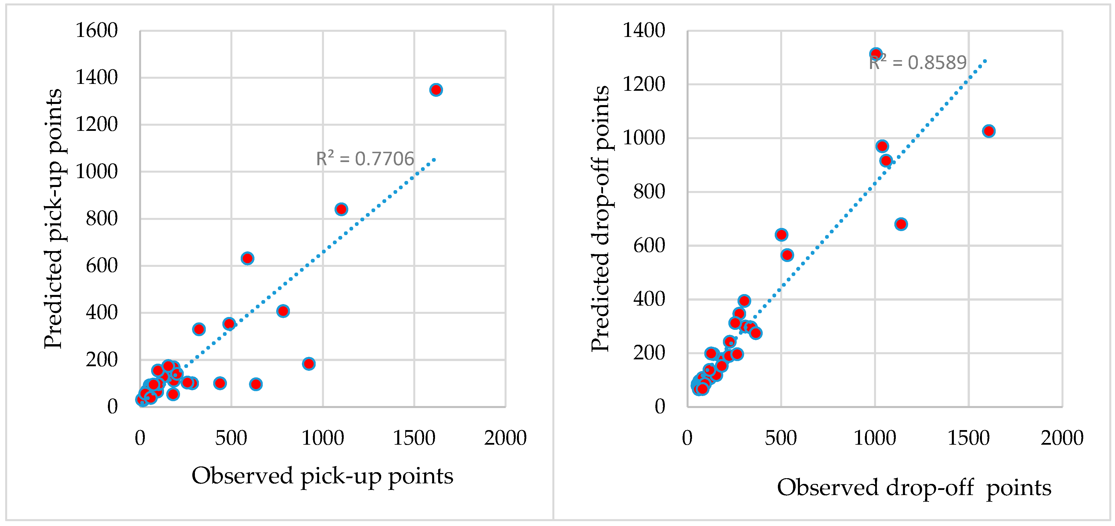
5.2. Identifying the Factors That Affect Population Movement

The main objective is to model the population movement pattern and to predict the population pattern for different regions, using the taxis’ origin and destination data. The Poisson regression model fits according to the parameters that impact the population movement. The results of pick-up and drop-off locations can be seen in Table 2 and Table 3, respectively. These tables provide the estimate of every independent variable’s coefficients in addition to the standard error and the p-value probability. According to these tables, each parameter’s role in impacting the population movement patterns is determinable. In these tables, B is the non-standard regression coefficient, and S.E is the standard error. The positive coefficients of the independent variables indicate with the increase in their values, the number of pick-up and drop-off locations in a neighborhood also increases. EXP (B) is equal to the predicted odds of the model. The prediction odds rate also indicates the ratio of a group’s frequency to the frequency of not-belonging to that class; when the value is less than 1, the odds of failure to winning are higher. The p-value can also be observed in the sig column. The sig column demonstrates the statistical significance and meaningfulness of the regression analysis model, in a way that, if the obtained result is less than 0.05, it is concluded that the utilized model is a good predictor of the pick-up and drop-off locations number variable. The output of this test is significant and meaningful concerning the p-value of 0.000 for the Poisson regression of the pick-up and drop-off locations. The main objective of this model is to investigate the effect of different parameters on the population movement pattern (the number of pick-up and drop-off locations). The p-value (Sig) for all variables in both pick-up and drop-off models is less than 0.05, and the null hypothesis for these variables is rejected. Therefore, the fitting of the Poisson model is significant and meaningful regarding all variables and these factors affect the population movement pattern and the number of pick-up and drop-off locations. Meaning that for each added educational land use to a neighborhood, the number of pick-up locations increases by approximately 6.7% and the number of drop-off locations increases by 4.3%, or by adding a residential land use, the number of pick-up locations decreases by 0.2% and the number of drop-off locations decreases by 0.1% for a neighborhood. The 95% confidence interval states that if the sampling is repeated 100 times and one hundred confidence intervals are produced, 95 intervals will include the study parameter and only five of these intervals will not include the average of this study. The confidence level here is 95%. Thus, we may encounter a confidence interval in 5% of cases that do not include the study parameter. Therefore, it should be stated that this interval is 95% likely to include the population parameter. The 95% confidence interval can be seen in Table 2 and Table 3. According to these tables, the intervals of 0.63–0.72 (0.09) for pick-up locations and 0.039–0.048 (0.09) for drop-off locations include the actual values of the number of pick-up and drop-off locations within the context of educational land use, with a probability of 95%. This means it is 95% certain that the average number of pick-up and drop-off locations for educational land uses are between 0.63–0.72 and 0.039–0.048, respectively. The confidence interval for both models includes a small range; thus, the accuracy of estimating the number of pick-up and drop-off points is high. Decreasing the confidence interval length increases the accuracy of the distance estimator. In this model, the variables of administrative and cultural land uses with the prediction rates of 1.102 and 1.142 have a greater impact on increasing the number of pick-up and drop-off locations in each neighborhood. Additionally, in the health-treatment section, the prediction rates of 0.983 and 0.991 have less impact on the number of pick-up and drop-off locations in each neighborhood. Table 4 presents the comparison criteria for pick-up and drop-off locations. The Log-Likelihood in the model for pick-up and drop-off locations is −5794.05 and −3412.24, respectively. The Log-Likelihood determines the weakness of the model’s prediction, indicating the fact that the smaller the absolute value of the model, the better the model is considered to be. The Akaike Information Criterion (AIC) is a measure of how well the fit index operates, and a model with the least AIC is considered the best. The Bayesian Information Criterion (BIC) is a tool in statistical calculations to select the best model from a limited number of models. The results obtained from the evaluation of the models using AIC and BIC criteria are similar to their values being close to each other [45]. The amount of AIC for pick-up and drop-off locations is 11616.11 and 6852.49, respectively, and the amount of BIC for pick-up and drop-off locations is 11648.37 and 6884.74, respectively. Therefore, according to Table 4, the Poisson regression model displays a better performance in terms of the number of drop-off locations. The expected number of pick-up and drop-off locations for each neighborhood can be determined based on the Poisson model, as a relationship between Equations (7) and (8), respectively, where xi is equal to the independent variables of the model and Ai is equal to the coefficients of the model.
λ i = e ( 4.35379 + i A i x i ) 0 i 13
λ i = e ( 4.31342 + i A i x i ) 0 i 13
To validate the Poisson regression model in modeling the number of pick-up and drop-off points, this model predicts the number of pick-up and drop-off points for areas not included in the modeling. In addition, the data in the research were divided into two categories, 60% for model training and construction and 40% for model testing and validation. The validity of the model is tested by comparing the observed and predicted number of pick-up and drop-off points in each neighborhood. The number of passenger pick-up and drop-off points is obtained using Equations (7) and (8). Figure 9 shows the predicted number of pick-up and drop-off points versus the observed number of pick-up and drop-off points.

6. Discussion

One of the aims of this study was to discuss the movement pattern of the population in the city of Bojnourd. Analyzing the movement pattern of a population can help analyze an unplanned event. The results of this study can guide city-related policies and urban planning to control urban traffic and detect high-risk areas of the Coronavirus and adopt policies to reduce densely populated areas. The number of trips absorbed and generated was calculated based on GPS city taxis. According to the results, the same pattern occurs every day for the trips produced and absorbed, and most trips take place in the city center. The pattern of population movement in Bojnourd is consistent with other studies conducted in Nanjing [29]. The number of trips produced and absorbed varies over time for each neighborhood. In this study, spatial autocorrelation was used for analysis. This analysis helps identify the peculiarity or randomness in the pattern of distribution of pick-up and drop-off locations. Besides, if a particular pattern is identified, it also helps pinpoint the areas with a meaningful density of points. In this regard, the results of the global Moran’s I index showed that the probability of random distribution of pick-up and drop-off locations is low. Additionally, the number of points and spatial distribution impacts Moran’s I index. Moreover, the global Moran’s I identifies only the type of pattern and cannot find the location of pick-up and drop-off clusters. Hence, the Getis-Ord-Gi statistic was used in illustrating the spatial distribution of the pick-up and drop-off locations and analyzing hot spots. The results of the study also showed that the probability of random distribution of pick-up and drop-off points is low. The spatial patterns indicated that in the time intervals between 8:00 to 9:00 and 14:00 to 15:00, the number of pick-up locations from downtown to the suburbs decreases, and the drop-off locations from the center to the suburbs increases. The hot spots of the pick-up in the central area follow the southeast of the cluster pattern. In other sections, these patterns are sparse and non-clustered. The hot spots of pick-up locations are more elongated than the hot spots of the drop-off locations and cover a larger portion of the study area. Additionally, hot spots of pick-up and drop-off locations are located in the urban downtown and Shahid, Sabzeh Square, Kargar Square, and Ferdowsi Square. By identifying the busiest areas during the day and night, in the central areas of the city, which are busy during the day, Corona testing can be done for free and instantly, and if possible, proper ventilation can be installed in these places. In addition, according to the parameters affecting the population distribution and the results indicate that the movement pattern has a significant relationship with land use. Given that commercial land use plays a major role in pick-up and drop-off locations, it is possible to build temporary stores to prevent crowds in central stores in crowded neighborhoods. Planning traffic facilities requires understanding the characteristics of urban travel and transportation. In this regard, coordination between traffic studies and urban planning is necessary. These programs can include long-term plans for road networks, transportation systems, parking lots, and terminals, as well as environmental impact assessments of changes in these plans.
Gong et al. (2015), Shen et al. (2017), and Yuan and Le Noc (2018) have studied and discovered population movement patterns based on GPS taxi data. The results of the mentioned research identified the location of people and the discovery of the movement pattern by calculating the number of generated and absorb trips. Rahimi et al. (2021) also modeled the spatiotemporal population with taxi data. In this study, using the generated and absorbed trips, the dynamic population was predicted. In most researches, big data of taxi origin and destination have shown good performance for spatial analysis, but in little studies, the parameters affecting the movement pattern have been studied to predict the number of absorbed and generated trips. Given the need to identify densely populated areas for urban planning and provide appropriate solutions, it is necessary to identify the factors affecting population movement. In this regard, the use of statistical analysis is novel and necessary, and desirable in any region. Therefore, another purpose of this study is to identify the factors affecting the distribution of population to predict the number of generated and absorb trips. The Poisson regression model is fitted to the parameters affecting the population distribution, the result of which shows that the model used is a good predictor for the variable of generated and absorbed trips. From the comparison of the number of observed and predicted trips, the coefficient of determination for the model (R2) was 0.77 and 0.85 for the pick-up and drop-off points, respectively. Regression analysis showed that the model works well for pick-up and drop-off points. Therefore, Equations (7) and (8) can be used effectively to analyze and predict pick-up and drop-off points. The reason for the difference in the prediction of pick-up and drop-off points can be various factors such as different economic and social characteristics in other neighborhoods.

7. Conclusions

This study examined the patterns of urban population displacement in Bojnourd based on taxi-driven data. Then, in the second part of the study, and by using regression analyzes, the parameters affecting the population movement pattern were modeled, and a model was presented in the way of predicting the population’s pick-up and drop-off locations.
Hourly distribution of pick-up and drop-off locations indicated the frequency of taxi-related travel throughout the day, and people take more taxis during the day than at night. Identification of population movement patterns by taxis’ origin and destination data has also been made in the research of Shen et al. [29] and Gong et al. [28]. The results of identifying the pattern of population movement for the study indicate that the distribution of pick-up and drop-off locations is not the same for different times and different land uses. In this study, spatial autocorrelation analysis was used to investigate the randomness or clustering of the number of pick-ups and drop-off points. The positive Moran index for the points of pick-up and drop-off indicates the spatial autocorrelation of the points.
The population movement patterns model should be utilized to determine the effect of each factor on the distribution of pick-up and drop-off locations. The role of various factors on the population movement patterns was calculated using the results of the Poisson regression model. The value of p for all variables in both the pick-up and drop-off locations is less than 0.05, and the null hypothesis for these variables is rejected. Therefore, the fitting of the Poisson model is significant and meaningful for all variables, and these factors affect the population movement pattern. Thus, the Poisson regression method is a good fitting method for population movement patterns data. The results of the modeling of the parameters affecting the population movement pattern indicate the effect of the administrative and cultural land uses on increasing the number of pick-up and drop-off locations in a neighborhood, which is due to the high volume of transporting different people to administrative and cultural centers during the day. Furthermore, medical land uses have the greatest effect on reducing the number of pick-up and drop-off locations in each neighborhood. According to the comparison criteria of Log-Likelihood, AIC, and BIC for pick-up locations (−5794.05, 11616.11, and 11648.37) and drop-off locations (−3412.24, 6852.49, and 6884.74), the Poisson regression model displayed a better performance for drop-off locations. It was indicated in the present study that according to the parameters of population, land use, migration, and area, it is possible to expand the appropriate modeling on the data regarding the origin and destination of taxis. Additionally, its results can be utilized in predicting the population movement pattern and the number of the people’s pick-up and drop-off locations. Given the p-value of 0.000, Poisson regression works well to model the effective parameters for population distribution. Comparison of predicted and observed values were also used for evaluation. The coefficient of determination for the model of the number of pick-up and drop-off points was 0.77 and 0.85, respectively, which could be due to differences in theeconomic and social characteristics of neighborhoods.
GIS, as a spatial information management system and spatial analysis, plays a valuable role in the analysis of taxis’ origin and destination data. Data-driven from taxis have great potential because of the use of massive amounts of data to identify citizens’ movement behavior, which, through spatial analysis, can be used to model movement patterns in urban areas. The findings of identifying the patterns of urban population mobility contribute to better urban transport management.
The method discussed in this paper is applicable in other cities to identify crowded areas and provide useful data for policymakers. In future studies, it will be possible to evaluate the travel behavior of individuals for specific activities and population estimation at any time. Nevertheless, to validate the results, comparison with other general information such as census and urban population information is important. Future research may include extending the study period to analyze seasonal time patterns when more data are available. Furthermore, the modeling of the parameters impacting the population movement patterns was conducted using Poisson regression, which produced significant results. However, other methods were provided for this modeling that can be utilized in future research.

Author Contributions

Conceptualization, A.S.-N.; methodology, F.R. and A.S.-N. and M.G.; software, F.R. and A.S.-N.; validation, A.S.-N. and M.G.; formal analysis, F.R. and M.G.; investigation, F.R. and A.S.-N.; resources, S.-M.C.; data curation, M.G.; writing—original draft preparation, F.R. and M.G.; writing—review and editing, A.S.-N. and S.-M.C.; visualization, F.R. and M.G.; supervision, A.S.-N.; project administration, S.-M.C.; funding acquisition, S.-M.C. All authors have read and agreed to the published version of the manuscript.

Funding

This research was supported by the MSIT (Ministry of Science and ICT), Korea, under the ITRC (Information Technology Research Center) support program (IITP-2021-2016-0-00312) supervised by the IITP (Institute for Information and communications Technology Planning and Evaluation).

Institutional Review Board Statement

Not applicable.

Informed Consent Statement

Not applicable.

Data Availability Statement

Not applicable.

Conflicts of Interest

The authors declare there are no conflict of interest.

References

  1. Aljoufie, M.; Zuidgeest, M.; Brussel, M.; Maarseveen, M. Urban growth and transport: Understanding the spatial temporal relationship. WIT Trans. Built Environ. 2011, 116, 315–328. [Google Scholar] [CrossRef] [Green Version]
  2. De Vos, O.; Witlox, F. Transportation policy as spatial planning tool; reducing urban sprawl by increasing travel costs and clustering infrastructure and public transportation. J. Transp. Geogr. 2013, 23, 117–125. [Google Scholar] [CrossRef]
  3. Lee, J. Reflecting on an Integrated Approach for Transport and Spatial Planning as a Pathway to Sustainable Urbanization. Sustainability 2020, 12, 10218. [Google Scholar] [CrossRef]
  4. Anagnostopoulou, E.; Urbancic, J.; Bothos, E.; Magoutas, B.; Bradeško, L.; Schrammel, J.; Mentzas, G. From mobility patterns to behavioural change: Leveraging travel behaviour and personality profiles to nudge for sustainable transportation. J. Intell. Inf. Syst. 2020, 54. [Google Scholar] [CrossRef] [Green Version]
  5. Wan, N.; Lin, G. Life-Space Characterization from Cellular Telephone Collected GPS Data. Comput. Environ. Urban Syst. 2013, 63–70. [Google Scholar] [CrossRef]
  6. Gao, S.; Yang, J.; Yan, B.; Hu, Y.; Janowicz, K.; Mckenzie, G. Detecting Origin Destination Mobility Flows from Geotagged Tweets in Greater Los Angeles Area. In Proceedings of the Eighth International Conference on Geographic Information Science (GIScience’14), Vienna, Austria, 24–26 September 2014. [Google Scholar]
  7. Rezende amaral, R.; Aghezzaf, E.; Raa, E.; Yadollahi, E. Adaptive Mobility: A New Policy and Research Agenda on Mobility in Horizontal Metropolises; In Planning; Department of Industrial Systems Engineering and Product Design: Groningen, The Netherlands, 2015; pp. 139–160. [Google Scholar]
  8. La Gatta, V.; Moscato, V.; Postiglione, M.; Sperlí, G. An Epidemiological Neural Network Exploiting Dynamic Graph Structured Data Applied to the COVID-19 Outbreak. IEEE Trans. Big Data 2021, 7, 45–55. [Google Scholar] [CrossRef]
  9. Mercorio, F.; Mezzanzanica, M.; Moscato, V.; Picariello, A.; Sperli, G. DICO: A Graph-DB Framework for Community Detection on Big Scholarly Data. IEEE Trans. Emerg. Top. Comput. 2019. [Google Scholar] [CrossRef]
  10. Wang, Y.; Qin, K.; Chen, Y.; Zhao, P. Detecting Anomalous Trajectories and Behavior Patterns Using Hierarchical Clustering from Taxi GPS Data. ISPRS Int. J. Geo-Inf. 2018, 7, 25. [Google Scholar] [CrossRef] [Green Version]
  11. Mazimpaka, J.D.; Timpf, S. Trajectory data mining: A review of methods and applications. J. Spat. Inf. Sci. 2016, 13, 61–99. [Google Scholar] [CrossRef]
  12. Sammer, G.; Saleh, W. Travel Demand Management and Road User Pricing: Success, Failure and Feasibility, 1st ed.; Routledge: London, UK, 2016. [Google Scholar]
  13. Jin, P.; Yang, F.; Cebelak, M.; Ran, B.; Walton, C. Urban travel demand analysis for Austin TX USAUrban Travel demand analysis for Austin TX USA using location-based social networking data. In Proceedings of the TRB 92nd Annual Meeting Compendium of Papers, Washington, DC, USA, 13–17 January 2013. [Google Scholar]
  14. Gemmer, M.; Becker, S.; Jiang, T. Observed monthly precipitation trends in China 1951–2002. Theor. Appl. Climatol. 2004, 77, 39–45. [Google Scholar] [CrossRef]
  15. Jin, P.; Cebelak, M.; Yang, F.; Zhang, J.; Walton, C.; Ran, B. Location-Based Social Networking Data: Exploration into Use of Doubly Constrained Gravity Model for Origin-Destination. Transp. Res. Rec. J. Transp. Res. Board 2014, 72–82. [Google Scholar] [CrossRef] [Green Version]
  16. Yang, C.; Clarke, K.; Shekhar, S.; Tao, V. Big Spatiotemporal Data Analytics: A research and innovation frontier. Int. J. Geogr. Inf. 2020. [Google Scholar] [CrossRef] [Green Version]
  17. Ge, W.; Shao, D.; Xue, M.; Zhu, H.; Cheng, J. Urban Taxi Ridership Analysis in the Urban Taxi Ridership Analysis in the Emerging Metropolis: Case Study in Shanghai. Transp. Res. Procedia 2017, 25, 4916–4927. [Google Scholar] [CrossRef]
  18. Jiang, B.; Yin, J.; Zhao, S. Characterizing the human mobility pattern in a large street network. Phys. Rev. E 2009. [Google Scholar] [CrossRef] [Green Version]
  19. Kheiri, A.; Karimipour, F.; Forghani, M. Intra-Urban Movement Patterns Estimation Based on Location Based Social Networking Data. J. Geomat. Sci. Technol. 2016, 6, 141–158. [Google Scholar]
  20. Gariazzo, C.; Pelliccioni, A.; Bogliolo, M.P. Spatiotemporal Analysis of Urban Mobility Using Aggregate Mobile Phone Derived Presence and Demographic Data: A Case Study in the City of Rome, Italy. Data 2019, 4, 8. [Google Scholar] [CrossRef] [Green Version]
  21. Yang, Z.; Gao, W.; Zhao, X.; Hao, C.; Xie, X. Spatiotemporal Patterns of Population Mobility and Its Determinants in Chinese Cities Based on Travel Big Data. Sustainability 2020, 12, 4012. [Google Scholar] [CrossRef]
  22. Wu, Y.; Wang, L.; Fan, L.; Yang, M.; Zhang, Y.; Feng, Y. Comparison of the spatiotemporal mobility patterns among typical subgroups of the actual population with mobile phone data: A case study of Beijing. Cities 2020, 100. [Google Scholar] [CrossRef]
  23. Rizwan, M.; Wan, W.; Cervantes, O.; Gwiazdzinski, L. Using Location-Based Social Media Data to Observe Check-In Behavior and Gender Difference: Bringing Weibo Data into Play. ISPRS Int. J. Geo-Inf. 2018, 7, 196. [Google Scholar] [CrossRef] [Green Version]
  24. Lyu, T.; Wang, P.; Gao, Y.; Wang, Y. Research on the big data of traditional taxi and online car-hailing: A systematic review. J. Traffic Transp. Eng. 2021, 8, 1–34. [Google Scholar] [CrossRef]
  25. Sun, Y.; Ren, Y.; Sun, X. Uber Movement Data: A Proxy for Average One-Way Commuting Times by Car. ISPRS Int. J. Geo-Inf. 2020, 9, 184. [Google Scholar] [CrossRef] [Green Version]
  26. Gong, S.; Cartlidge, J.; Bai, R.; Yue, Y.; Li, Q.; Qiu, G. Extracting activity patterns from taxi trajectory data: A two-layer framework using spatio-temporal clustering, Bayesian probability and Monte Carlo simulation. Int. J. Geogr. Inf. 2019. [Google Scholar] [CrossRef] [Green Version]
  27. Yuan, Y.; Le Noc, M. Exploring Urban Mobility from Taxi Trajectories: A Case Study of Nanjing China. DATA 2018 2018. [Google Scholar] [CrossRef]
  28. Gong, L.; Liu, X.; Wu, L.; Liu, Y. Inferring trip purposes and uncovering travel patterns from taxi trajectory data. Cartogr. Geogr. Inf. Sci. 2015. [Google Scholar] [CrossRef]
  29. Shen, J.; Liu, X.; Chen, M. Discovering spatial and temporal patterns from taxi-based Floating Car Data: A case study from Nanjing. GIScience Remote Sens. 2017. [Google Scholar] [CrossRef]
  30. Rahimi, F.; Sadeghi-Niaraki, A.; Ghodousi, M.; Choi, S.-M. Modeling Population Spatial-Temporal Distribution Using Taxis Origin and Destination Data. Sustainability 2021, 13, 3727. [Google Scholar] [CrossRef]
  31. Hataminezhad, H.; Poorahmad, A.; Mansourian, H.; Rajaei, S.A. Spatial Analysis of Quality of Life Indicators in Tehran City. Hum. Gegraphy Res. Q. 2014, 45, 29–56. [Google Scholar]
  32. Saraei, M.H.; Chaharrahi, A.; Safarpour, M. Study and Analysis of Spatial Distribution of Hotels toward the Tourism Attractions Case Study: Shiraz City. Geogr. Territ. Spat. Arrange 2016, 6, 171–182. [Google Scholar]
  33. Saddam Hussain, M.; Jha, D.; Goswami, A.K. Using GIS to identify vehicle crash hot spots and unsafe crossroads-a case study of Kolkata, India. In Proceedings of the Asian Conference on Remote Sensing, Kuala Lumpur, Malaysia, 15–19 October 2018. [Google Scholar]
  34. Ahmadi, M.; AliMohammadi, A. Accidents Prediction Using Multilevel Regression Model and Time Parameters. Traffic Law Enforc. Res. Stud. 2015, 2015, 105–138. [Google Scholar]
  35. Dinu, R.; Veraragavan, A. Random parameter models for accident prediction on two-lane undivided highways in India. J. Saf. Res. 2011, 42, 39–42. [Google Scholar] [CrossRef]
  36. Zhao, P.; Xu, Y.; Liu, X.; Kwan, M. Space-time dynamics of cab drivers’ stay behaviors and their relationships with built environment characteristics. Cities 2020, 101. [Google Scholar] [CrossRef]
  37. Zhou, T.; Liu, X.; Qian, Z.; Chen, H.; Tao, F. Dynamic Update and Monitoring of AOI Entrance via Spatiotemporal Clustering of Drop-Off Points. Sustainability 2019, 11, 6870. [Google Scholar] [CrossRef] [Green Version]
  38. Wang, Z.; Fang, C. Spatial-temporal characteristics and determinants of PM2.5 in the Bohai Rim Urban Agglomeration. Chemosphere 2016, 148–162. [Google Scholar] [CrossRef]
  39. Fang, C.; Wang, Z.; Xu, G. Spatial-temporal characteristics of PM2.5 in China: A city-level perspective analysis. J. Geogr. Sci. 2016, 26, 1519–1532. [Google Scholar] [CrossRef]
  40. Esri. Available online: http://resources.arcgis.com/en/help/main/10.2/index.html#//005p00000006000000 (accessed on 10 April 2016).
  41. Shahbazi, H.; Taghvaee, S.; Hosseini, V.; Afshin, H.A. GIS based emission inventory development for Tehran. Urban Clim. 2016, 17, 216–229. [Google Scholar] [CrossRef]
  42. Pahlavani, P.; Sheikhian, H.; Bigdeli, B. Assessment of an air pollution monitoring network to generate urban air pollution maps using Shannon information index, fuzzy overlay, and Dempster-Shafer theory, A case study: Tehran, Iran. Atmos. Environ. 2017, 254–269. [Google Scholar] [CrossRef]
  43. Ord, J.K.; Getis, A. Local spatial autocorrelation statistics: Distributional issues and an application. Geogr. Anal. 1995, 27, 286–306. [Google Scholar] [CrossRef]
  44. Washington, S.; Karlaftis, M.; Mann, F. Statistical and Econometric Methods for Transportation Data Analysis; Chapman & Hall/CRC: Boca Raton, FL, USA, 2003. [Google Scholar]
  45. Oyindamola, B.Y.; Linda, O.U. On the Performance of the Poisson, Negative Binomial and Generalized Poisson Regression Models in the Prediction of Antenatal Care Visits in Nigeria. Am. J. Math. Stat. 2015. [Google Scholar] [CrossRef]
Figure 1. The study area.
Applsci 11 05987 g001
Figure 2. The stages of research.
Applsci 11 05987 g002
Figure 3. Spatial distribution of pick-up and drop-off zones.
Applsci 11 05987 g003
Figure 4. The pick-up and drop-off locations statistics in the different time scales.
Applsci 11 05987 g004aApplsci 11 05987 g004b
Figure 5. Spatial distribution of pick-up and drop-off locations for November and December.
Applsci 11 05987 g005aApplsci 11 05987 g005bApplsci 11 05987 g005c
Figure 6. Spatiotemporal distribution of pick-up and drop-off locations.
Applsci 11 05987 g006aApplsci 11 05987 g006bApplsci 11 05987 g006c
Figure 7. Hot spots and cold spots for pick-up and drop-off locations.
Applsci 11 05987 g007aApplsci 11 05987 g007bApplsci 11 05987 g007cApplsci 11 05987 g007d
Figure 8. Moran index changes over time.
Applsci 11 05987 g008
Figure 9. Predicted pick-up and drop-off points compared to observed.
Applsci 11 05987 g009
Table 1. A sample record of the data set.
Record ID204834129
Taxi ID121
Longitude57.3349
Latitude37.4843
Velocity (KM/h)41
Direction-
Cost (Rial)1350
Status1
Table 2. Poisson regression model for pick-up locations.
ParameterBStd. Error95% Wald Confidence IntervalHypothesis TestExp (B)
LowerUpperWald Chi-SquaredfSig.
(Intercept)4.3540.02064.3134.39444,505.01110.00077.773
Area3.416 × 10−73.2644 × 10−82.776 × 10⁻⁷4.056 × 10⁻⁷109.50110.0001.000
Statistical_population0.0001.1083 × 10⁻⁵0.0000.000193.21910.0001.000
Migration0.0014.2259 × 10⁻⁵0.0010.001438.90210.0001.001
Administrative_land use0.0970.00210.0930.1012234.89610.0001.102
Educational_land use0.0670.00210.0630.0721053.62510.0001.070
Health_land use−0.0170.0018−0.021−0.01493.45510.0000.983
Commercial_land use0.0070.00010.0060.0072767.64110.0001.007
Industrial_land use−0.0020.0007−0.0040.00010.38710.0010.998
Cultural_land use0.0530.01260.0280.07817.82610.0001.055
Green_space_land use0.0760.00440.0680.085298.92210.0001.079
Religious_land use0.0390.00440.0310.04878.76210.0001.040
Sports_land use0.0300.00990.0110.0499.28410.0021.030
Residential_land use−0.0027.4203 × 10⁻⁵−0.002−0.001414.60010.0000.998
(Scale)1a
Table 3. Poisson regression model for drop-off locations.
ParameterBStd. Error95% Wald Confidence IntervalHypothesis TestExp (B)
LowerUpperWald Chi-SquaredfSig.
(Intercept)4.3130.02074.2734.35443,234.60810.00074.696
Area5.547 × 10⁻⁷3.0795 × 10⁻⁸4.944 × 10⁻⁷6.151 × 10⁻⁷324.48310.0001.000
Statistical_population0.0001.0729 × 10⁻⁵9.709 × 10⁻50.000121.20910.0001.000
Migration0.0014.1761 × 10⁻⁵0.0010.001932.81210.0001.001
Administrative_land use0.0820.00230.0780.0871271.76710.0001.086
Educational_land use0.0440.00240.0390.048343.45110.0001.045
Health_land use−0.0090.0015−0.012−0.00640.01310.0000.991
Commercial_land use0.0060.00010.0050.0061663.57210.0001.006
Industrial_land use0.0030.00070.0010.00415.77010.0001.003
Cultural_land use0.1330.01350.1060.15996.72210.0001.142
Green_space_land use0.0670.00490.0580.077191.87010.0001.070
Religious_land use0.0390.00480.0290.04864.29110.0001.039
Sports_land use0.0200.01010.0000.0403.97510.0461.020
Residential_land use−0.0017.2069×10⁻⁵−0.002−0.001412.91810.0000.999
(Scale)1a
Table 4. Comparison criteria for pick-up and drop-off locations.
Log LikelihoodAIC 1BIC 2
Number of pick-up locations−5794.0511,616.1111,648.37
Number of drop-off locations−3412.246852.496884.74
1 Akaike Information Criterion 2 Bayesian Information Criterion.
Publisher’s Note: MDPI stays neutral with regard to jurisdictional claims in published maps and institutional affiliations.

