1. Introduction
During the last few years, the presence of renewable energy generation has increased significantly within power systems [
1]. These renewable generators are usually organized as small, mini, or micro power plants, but they are also used as complementary generation devices for consumers. Notably, the increasing presence of renewables marks a large change from a traditional centralized generation system to a distributed system. This trend is based on the distributed generation (DG) paradigm [
2]. This paradigm is one of the key points in the smart grid sector [
3,
4,
5] and is characterized by better control of all connected resources (including consumers and producers) and other goals [
6], coverage of the whole system, and the application of artificial intelligence techniques [
7].
In the DG paradigm, active sources are connected directly to the distribution network, permitting them to be nearer to consumption points [
8]. These elements are usually called distributed energy resources (DERs). Moreover, the DER concept is not only associated with generation systems [
9] but also with the coverage of storage [
10,
11] and even controllable loads [
12,
13]. In this sense, electric vehicles (EVs) can also be considered DERs, adding to the difficulty of being a mobile load [
14,
15,
16]. Traditionally, all these DERs have been coordinated by energy management systems (EMSs).
Moreover, driven by current regulations [
17], there is expected to be a rising tendency toward the close participation of consumers in electricity and flexibility markets through tools such as demand response (DR) services [
13]. These markets could include aggregator participation to simplify the management of resources [
18].
Based on the aforementioned context, it can be identified that good forecasting of power generation and consumption is essential at various network levels. For example, transmission system operators (TSOs) and distribution system operators (DSOs) use forecasting to perform power system operation tasks [
19,
20]. Even the mentioned EMSs in customer installations usually require the forecasting of some power consumption or generation metrics to optimize the use of resources under different criteria. These can be related to energy efficiency in buildings [
21] and microgrids [
22], environmental and economic improvements [
23], or even the control of active and reactive power [
24].
Based on this need, a complete framework for the multistep short-term forecasting of electric power consumption and generation is proposed in this paper. Unlike other common approaches found in the existing literature, the proposed framework performs day-ahead forecasting at the start of the day without requiring online training. If online training is used, where the observations from each day are used to update the model [
25] (this is also called “incremental learning”), the daily computational cost needs to be considered to guarantee the applicability of the method [
26].
Regarding the techniques for forecasting models, this framework proposes the use of rule-based baselines or two machine learning techniques; a multi-layer perceptron regressor (MLPR) and a random forest regressor (RFR).
The rule-based baseline methods include the proposal and definition of different rules, where the number of previous days to be used can be specified, as well as whether any distinction by day type will be applied. Despite baseline methods being typical and classical prediction methods (some examples can be found in [
27,
28,
29]), an important number of variations and specifications are proposed and evaluated here, and these yield the best results.
These proposed baseline models have been found to be useful not only as nonblack-box methods but also as possible inputs for machine learning techniques. In this sense, the previously proposed machine learning techniques have been evaluated under different combinations of inputs, identifying which input sets achieve better results. Among the evaluated input variables, the cross relationship between the power variables under study has also been considered and exploited to improve the forecasting results. The inclusion of this information is performed using what is called an “external baseline” (EXBL), i.e., adding a baseline of some other variable of the microgrid (e.g., load consumption) as an input of a machine learning method; this idea is one of the proposals of the present paper.
The methodology of the proposed framework is applied in a study case to forecast five different power variables (load, generation metrics of various types, and others) for the Savona Campus of the University of Genoa in Italy.
The rest of the paper is organized as follows:
Section 2 reviews state-of-the-art forecasting techniques for generation and load consumption.
Section 3 presents the utilized methodology, which is applied in the framework proposed in
Section 4.
Section 5 presents the details of the case study, whose results are described in
Section 6. Finally, the conclusions are depicted in
Section 7.
2. State-of-the-Art Methods
In the field of power forecasting, a wide variety of techniques and methods have been proposed in the literature, and their ambit of application depends on the characteristics of the forecast, such as the time aggregation and horizon of prediction.
The two main types of forecasting are deterministic and probabilistic methods. Deterministic forecasting results in point outputs, with one value at each step, while probabilistic forecasting assigns probabilities to the various scenarios; these can be in the form of quantiles, intervals, or density functions [
30]. Both approaches are used in related existing methods to obtain probabilistic forecasts from deterministic methods, such as bootstrapped prediction intervals (BPIs) and quantile regression averaging (QRA) [
31].
Regarding deterministic methods, an extensive summary of the different forecasting approaches can be found in [
32], where the authors review different electrical load forecasting methods and analyze their convenience according to the time aggregation, the time required for forecasting and the most convenient type of data used as input. In particular, the analysis covers 113 different case studies reported across 41 academic papers. The different methods are categorized as “regression” methods, “bottom up” approaches, “artificial neural networks” (ANNs), “support vector machines”, “time series analysis” methods, and other techniques used in mid-term forecasting. Additionally, several tables and graphs are provided to show the situations in which these methods are most popular.
Reference [
30] contains a review of the applications of probabilistic methods in load forecasting. Despite these methods being of great interest, they present some additional problems from the point of view of their evaluation processes, as the typical metrics used for deterministic methods are not valid due to the existence of quantiles, prediction intervals or confidence intervals. This is why some authors have proposed metrics such as the pinball score or the Winkler score [
30,
33].
Due to these additional difficulties and considering that many energy management applications are based on deterministic forecasts (for example, the abovementioned approaches [
22,
23,
24]), the present paper is focused on deterministic methods, with the inclusion of probabilistic techniques being a future research topic.
The types of techniques that can be found in the literature are dependent on the ambit of application, such as the customer level, building level, renewable generation units, microgrids of diverse sizes, distribution networks, or even market level (e.g., price forecasting [
31]).
In [
34], J. Runge and R. Zmeureanu review the use of ANNs for forecasting energy use in buildings. A list of found methods that select hyperparameters is also detailed, including (i) heuristics (such as rules of thumb), (ii) cascade correlation, (iii) evolutionary algorithms (EA) and (iv) automated architectural search. The comparison of reviewed papers includes information about the time steps, forecast horizons, and error metrics used by these methods. Other details about the limitations of ANN-based forecasting are explained.
As previously mentioned, the influence of weather conditions is of high importance due to the increasing use of renewable generation, such as solar and wind plants, which present power generation effects that change with atmospheric conditions. For this reason, many authors have studied how to consider these conditions to improve forecasting methods. In this sense, reference [
35] contains recommendations for the use of weather data in microgrid-related forecasts. The authors especially recommend using real forecast data (received from a public or commercial forecasting service) for modeling, not any other synthetic dataset (i.e., data specifically designed for the given experiment with different degrees of similarity relative to reality). The importance of clearly defining the error metrics to be applied is also pointed out.
Regarding wind power generation, some approaches followed in existing studies for short-term and ultrashort-term forecasting include the use of autoencoders and back propagation [
36], numerical weather prediction [
37], and long short-term memory (LSTM) [
38,
39]. Thus, other approaches apply wavelet decomposition combined with machine learning techniques [
40].
In the field of photovoltaic generation, one study [
33] presents a method for probabilistic forecasting based on LSTM and quantile regression averaging (QRA). A 24-h-ahead forecasting method based on synthetic weather forecasting and LSTM is applied in [
41].
In applications that are more focused on small customer forecasting, which mainly includes load consumption, customer segmentation by type is a very common approach. In [
42], customers were divided into clusters to model and forecast the next 12 h of consumption. The existence of photovoltaic generation on the customer side and its effect on total consumption are also considered in [
43]. In [
44], a comparison of techniques was performed over a single household using one month of data, showing the superiority of machine learning techniques over linear regression. The inclusion of appliance (dishwashers, televisions, etc.) measurements have been shown to be useful for discovering resident behaviors and improving forecasting results, as described in [
45].
Some examples of studies including buildings with greater consumption (such as universities) can also be found in the literature. A study of power consumption forecasting on a university campus is presented in [
46] using conditional linear predictions. The authors compare the performance of a method using between 1 and 96 bins (the number of divisions in which a day is divided for forecasting), showing how an 8-bin division achieves more accurate performance than the use of 96 bins. In [
47], Y. Ding et al. present a prediction model for campus buildings based on occupancy patterns. This is a good example of how knowledge of building use can be of great interest for consumption prediction.
Finally, regarding applications at the distribution network level, ANNs are applied in [
48] to predict the maximum demand response over a secondary distribution network in India. The aim is to avoid violations of the permitted contractual demand limit by utilities. The study of consumption peaks is of particular interest for congestion management applications. Due to their importance and their difference from other more general forecasts, some authors have proposed specific methods and evaluation metrics for peak predictions, as in [
49], where the proposed metric reduces penalization in cases of peak deviations between the real data and the forecasts.
Many of these papers propose the use of artificial intelligence techniques, such as those used in the present paper, to perform forecasting. This type of method has been shown to obtain better results than other classical methods (such as statistical methods) in many situations. However, it is worth mentioning that in some cases, artificial intelligence methods constitute black-box models, so their behaviors sometimes cannot be easily explained.
In this regard, some authors have proposed the use of rule-based methods that introduce expertise-based knowledge to permit the extrapolation of models in some cases [
50] or that substitute black-box models by others that are more understandable [
51].
Another type of forecasting model includes baselines, which are frequently obtained from the measurements taken on some previous similar days [
30,
49] or from similar groups of customers [
52]. In the context of new flexible service applications, baseline models could be considered good approaches for obtaining the expected consumption levels of customers, making it possible to evaluate their availability and audit their performance in flexible service scenarios. This interest is clearly stated by the European Commission in [
53]: “Since flexibility (by definition) cannot be measured, a baseline is needed to quantify the delivered flexibility”. They also point out some recommendations regarding the design and implementation of baselines, such as the avoidance of inaccurate or biased baselines. Complex baseline methodologies could also impact the reproducibility, transparency, and implementation costs [
53] of the processes. Despite the interest that these methods have generated, in many studies, they are usually reserved for conducting performance comparisons with more complex models (i.e., used as reference methods).
In this sense, while artificial intelligence methods have been shown to be particularly useful and accurate for consumption prediction, many of their techniques are based on black-box models. This fact becomes a drawback in some situations, such as in auditory processes or agreements (as, for example, in [
54]), as poor interpretability could result in nontransparent contracts, where the expected consumption or generation could be biased due to the intrinsic nature of the AI model. Therefore, the present paper proposes various rule-based baselines that are simple to understand and apply in the context of a transparent contract.
Additionally, these proposed baselines are also used as inputs for more complex machine learning methods (random forests and neural networks), thereby improving the quality of the obtained forecast according to the results.
Notably, the methodology to be applied depends on the characteristics of the time horizon and the aggregation of the forecasting data. Specifically, the methodology and framework proposed in the present paper are oriented to day-ahead multistep forecasting.
3. Methodology
As mentioned above, power forecasting is needed in multiple applications, such as obtaining the available flexible capacity for a customer, performing grid management tasks based on expected customer behavior, or improving the daily optimization of resources with an EMS. In this sense, a framework for forecasting electric power variables (generation/consumption) is proposed here. This framework has the objective of modeling the power values of a system for all timeslots in a given day.
This forecasting could be achieved by developing a one-output model that gives a prediction for the selected time interval (or time step) with every execution or a multiple output model that gives predictions for all the intervals in a day with one execution of the model.
Referring to time and performance criteria, the best approach would be to use multioutput models, which utilize a lesser amount of data for the training and testing processes (each dataset contains all the outputs for one day). In contrast, a one-output model is fed with every independent value for each interval of the available days, requiring more time for training and testing.
Two main approaches are proposed here for modeling: rule-based baselines and artificial intelligence regression methods (which also consider the inclusion of baseline forecasts as additional inputs).
3.1. Rule-Based Baseline Prediction
A baseline consists of a forecast of a power variable based on previous measurements of that variable. This method can be applied by following different rules depending on what the objective is and the type of days and events that could be identified during the period of interest. In this sense, a common approach is to distinguish only between weekdays and weekends, but in this work, this technique is extended by the definition and specification of different rules that can be chosen depending on the type of variable to forecast.
Specifically, these proposed models perform multistep day-ahead predictions for a whole day using only the historical data obtained on some previous days. The number of days to be used is defined by the integer
n, which is the parameter that establishes the model configuration (therefore, it will hereinafter be referred to as a hyperparameter) depending on the rule to be applied. Once the days to be used are selected, the mean power value is calculated for each of the time intervals of those days, with these values being the forecasts for these days. This process is depicted in
Figure 1.
The four types of proposed baseline rules are as follows:
Baseline “simple n” (abbreviated as baseline_sn): This rule takes the n days prior to the target day and calculates the mean for each time interval. There are no day-type distinctions with this rule. The proposed values for n are 1, 2, 3, 4, 5, 6, 7, 14, 21, 28, and 35.
Baseline “basic_weekend n” (abbreviated as baseline_bwn): In this rule, n days before the objective day are considered, but not all of them are used in the baseline calculation. If the objective day is a weekend day, the weekend days within the previous n days are averaged for each interval of each day. The same situation occurs if the objective is a nonweekend day, where all nonweekend days within n days are taken. The proposed values for n are 7, 14, 21, 28, and 35.
Baseline “const_num_back n” (abbreviated as baseline_cnbn): This rule takes n days before the objective day, which are of the same type; i.e., if the objective is a weekend day, n previous weekend days are taken. The proposed values for n are 1, 2, 3, and 4.
Third item. Baseline “same_weekday n” (abbreviated as baseline_swn): In this rule, from n days before the objective day, only those that are the same day of the week are used in the baseline calculation. For example, if the objective day is a Tuesday, the Tuesdays included in the set of n days are averaged for each time interval. The proposed values for n are 7, 14, 21, 28, and 35.
Thus, the proposed values for the hyperparameter n are not the same for all rules. The selection of those values is due to the nature of each rule and the set of days that can be obtained. In the case of the “basic_weekend” and “same_weekday” rules, only multiples of seven are taken to ensure the availability of days of the needed type inside the set of n days (seven days contains two weekend days and five nonweekend days). Taking another value for n would result in an irregular distribution of days, so this is avoided by taking only multiples of seven.
In the case of the rule “const_num_back”, the maximum value of n is four to avoid mixing data from different numbers of days back with respect to weekends (two weeks ago for n = 4) and non-weekends (one week ago for n = 4). If n is higher than four, a minimum of three weeks will be needed to calculate the baseline of a weekend day, which would be undesirable.
The
baseline_s1 method (the simple
n rule, where
n = 1) could be considered the simplest rule, so can be used as the reference method for comparison with the other rules. This idea is, for example, exposed in [
55], where it is mentioned that one of the most commonly used base methods is the naïve method [
55]. This method consists of using the last observation as the next prediction. Therefore, the
baseline_s1 method can be considered equivalent to the naïve method in this methodology, with day-ahead forecasting being the objective. This method is applied in [
43,
56,
57], where forecasting performed simply by using the measurements of the previous day was called the “persistence method”. Other authors propose the use of other methods, such as the autoregressive moving average (ARMA) [
43] or the autoregressive integrated moving average (ARIMA) models [
58], as references in their case studies. In the proposed methodology, the
baseline_s1 method is preferred because of its simplicity, as it avoids a more complex parameter adjustment process which would be required for other models such as ARMA or ARIMA (which would be computationally expensive due to the high orders of the models with data aggregations of 1 h or 15 min).
Once the rules are defined, their application can be classified into the “strict” and “non-strict” types.
The “strict application of a rule” implies that a baseline for a certain day is considered valid only if the available number of days in the set n is the maximum number defined by the rule. If there are any missing data in the needed days according to the rule, this baseline is discarded and not considered valid.
In contrast, the “non-strict application of a rule”, does not necessarily require a specified number of days. The baseline is considered valid if there is at least one day available for the calculation.
As will be seen in the case study, the evaluation of baselines will be performed under the criterion of strict application. Notwithstanding, some non-strict results will also be shown for illustrative purposes.
3.2. Neural Network Regressor
Among the numerous types of existing ANNs [
59], one of the most commonly used approaches for regression purposes is the MLPR [
60]. It is a powerful tool for predicting continuous variables, thereby supporting multioutput regression. This architecture is selected for the proposed architecture due to its relative simplicity and because it is less computationally expensive than other ANN types, such as recurrent neural networks (RNNs).
The basic structure of an MLPR with a single hidden layer can be seen in
Figure 2. A similar structure is adopted if more than one hidden layer is added.
For the proposed architecture, a multilayer perceptron (MLP) that conducts training using backpropagation [
61] is used. The activation function in the hidden layers is the rectified linear unit (ReLU) function (1), which has a lower computational cost than other activation functions, such as the logistic or hyperbolic tangent functions. In contrast to the MLP used for classification, the activation function in the output layer is the identity function, achieving continuous values for the outputs (a regression behavior). Furthermore, the squared error is used as the loss function during training.
Thus, as is usually recommended, parameter regularization techniques are applied to obtain better generalized models [
62] (reducing the probability of overfitting during the training process). This means that weights with large magnitudes are penalized during training, so large values are not retained (they are regularized). Two well-known techniques for this purpose are lasso regression (ℓ1) and ridge regression (ℓ2) [
62]; the penalty term is squared in ℓ2 (which brings higher sensitivity to high weight values). For this reason, the ℓ2 technique is preferred. The regularization effect is adjusted by a hyperparameter called “alpha”.
The use of an MLPR for modeling requires deciding the number of hidden layer neurons (hyperparameter
nh) to be used. In this sense, some authors have proposed heuristics (rules of thumb) to select the number of hidden neurons [
34]. Their expressions are shown in (2)–(7):
nh indicates the number of hidden layer neurons;
ni is the number of input neurons;
no is the number of output neurons;
l is an integer between 1 and 10; and
N is the number of training samples.
Considering the characteristics of each input and output dataset (their sizes), it is possible to directly calculate the recommended number of hidden neurons according to these rules. These recommendations are used to obtain initial estimations of the range of nh values that will be tested during the experiments.
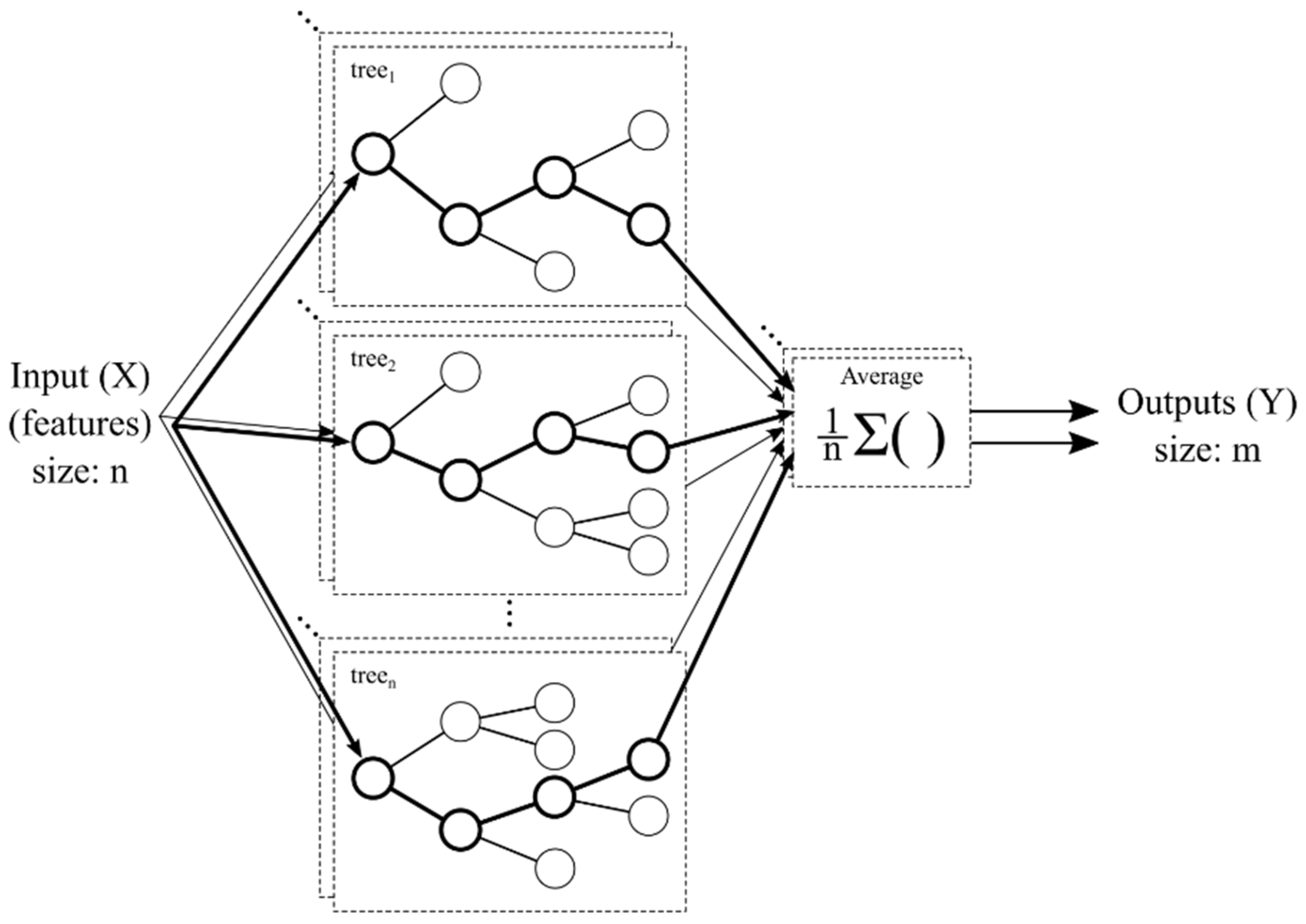
3.3. Random Forest Regressor
A random forest [
63] is based on splitting the input dataset into multiple groups and training a decision tree for each of these groups. Finally, the results of each tree are passed to a voting block (in this case a random forest for classification) or an averaging block (for regression), obtaining an RFR in the second case. One of the main hyperparameters of an RFR is the number of trees to use. A higher number can improve the performance of the model, but the computational cost grows linearly with the increase in the number of trees.
The structure of an RFR is shown in
Figure 3. It can be used for single-output or multioutput prediction simply by adding new tree structures for each of the desired outputs.
In the proposed framework, the datasets for both artificial intelligence regression methods (the MLPR and RFR) are the same, as both models are configured to be multioutput prediction methods.
3.4. Forecasting Performance Metric
Which indicator to use for comparing the obtained forecasting errors is a very common topic of discussion in the literature. In [
64], a summary of possible indicators can be found.
In classical approaches, the mean average error (
MAE), root mean square error (
RMSE) and coefficient of determination (R
2) are considered useful for the evaluation of model performance. Furthermore, there are other widely used indicators, such as the mean average percentage error (
MAPE) [
34]. However, the
MAPE is not convenient for predicting certain variables that contain positive and negative values, which may exist in a distribution network that includes generation resources. In these situations, the
MAPE tends to yield very large values due to the existence of zero or low values in the data to be predicted, and this could lead to misunderstanding in their interpretation. Finally, the main indicator used for the comparison of model performances is the coefficient of variation of the root mean square error (
CV(
RMSE)) [
34,
64], also called the relative root mean square error (
RRMSE) by some authors (i.e., [
65]). This indicator has the disadvantage of yielding higher forecasting error values than those of other indicators when the variable to be predicted has a low average value (as highlighted in [
33]), but it avoids the appearance of very high (or even infinite) values in near-zero samples.
Another metric that is defined here due to its simplicity is the normalized
RMSE (
nRMSE). While its definition can vary from one author to another [
66], here, it is considered equal to the
RMSE divided by the capacity of generation (in cases with generation resources) or by the capacity of consumption (in cases with loads).
The expressions of the abovementioned metrics are shown in (8)–(12):
Furthermore, many other indicators can be found in the literature. The authors in [
35] point out the importance of using well-defined indicators as error metrics. One of the main problems faced when comparing the forecasting results of different studies is precisely the absence of error metric standardization. This ambiguity is particularly noticeable in normalized indicators such as the normalized
MAE (
nMAE) or normalized
RMSE (
nRMSE).
For other applications, some authors propose more specific metrics to emphasize certain aspects of the resulting forecast, such as consumption peaks. For example, the authors in [
49] propose a “semi-metric” approach to avoid the double penalty effect when a forecasted peak deviates in time from the real peak. This approach is useful for applications specifically centered on peak reductions at the network level; as for these applications, it is more important that peaks be predicted at approximately the correct times rather than not at all. However, for general applications in energy management, it is preferable to follow some of the common indicators that were previously described, as most of the authors do in the reviewed bibliography (for example, [
44,
45,
47]). Therefore, this is the approach adopted in the present study.
After analyzing the advantages of each indicator, the CV(RMSE) was finally chosen, as it is appropriate for the evaluation of a series with both positive and negative values.
4. Proposed Framework
In the field of power forecasting, it is common to use datasets that, apart from power values (with their corresponding timestamps), also include weather information such as temperature and humidity data. Moreover, this information can (and should) be enriched with the inclusion of extra information. This additional information could be date-related information (e.g., days of the week, workdays) or the inclusion of previous measurements (e.g., the raw measurements taken on some previous days). Furthermore, as part of the proposals of the present paper, it is possible to include not only the raw data of previous days (which is usually done by other authors) but also their corresponding baseline forecasts obtained with the previously described rule-based baseline method.
Specifically, up to five groups of possible inputs (described in
Table 1) are proposed for this framework. The exact number of inputs in some of these groups depends directly on the aggregation of the forecasted variable (the number of time intervals considered in a whole day) and the aggregation of weather forecasts (which could be different from the aggregation of the forecasted variable).
Day information includes representative data about the date, such as the year, the month, and the day of the week.
The external baseline (EXBL) consists of a variable baseline that is different from the objective to be predicted (i.e., not the target variable but another variable of the microgrid, such as the load consumption). The reason for this inclusion is to take advantage of the correlations between the different variables (i.e., load consumption and the variable to be predicted) of the microgrid to improve the forecasting results. The datasets that include an EXBL are identified on their tags at the end of their names.
From the combinations of all these fields, multiple datasets can be generated to train models. In this sense,
Table 2 summarizes the different datasets proposed for this forecasting framework. To simplify the identification of the datasets, a tag (“dataset type”) is assigned to those similar datasets. Each tag summarizes the information included in the datasets (calendar information, weather, previous measurements, etc.) using a simple, short name.
One of the steps inside the proposed framework is to select which of the provided datasets is most convenient to perform forecasting.
The total number of inputs and outputs for a dataset, as previously described, depends on the aggregation level. Specifically, 15-min aggregations have 96 outputs for a whole day, while 60-min aggregations possess 24 outputs. The same is true for the other input fields that include measurements of previous days or baselines, where each input day implies the same number of inputs (96, 24, etc. according to the aggregation).
Based on the reviewed state-of-the-art methods and considering the typical needs of the mentioned applications, the aggregation levels are typically 15 min, 1 h and (in some cases) 2 h. This means that the number of time intervals (also called bins, time periods, or timeslots, depending on the author) is equal to 96, 24 or 12 for a whole day, respectively. The architecture is designed to perform multistep predictions at 00:00 of each day, obtaining a prediction for each variable for the next 24 h (day-ahead) under the desired aggregation level.
The general process is depicted in
Figure 4. The dataset preparation block receives information regarding the selected measures and weather data. These fields of information are formatted and combined to create the previously described datasets. In the model training/execution block, the three modeling techniques (the baseline, RFR and MLPR) train models using each of the datasets. At this point, as indicated in
Figure 4, the baseline models are used as feedback for the dataset creator and included as input groups (the baseline and external baseline) in some of the datasets (see
Table 2).
The trained models are then evaluated and ordered according to their performance metrics. The best models and their characteristics are stored in a database and are used by the daily forecasting block, which executes the best available model once a day (obtaining the day-ahead forecast). Notably, in this process, the type of information needed to execute each of the models must be specified, as the system must check the availability of the information before deciding which model to use. For example, if the temperature information is missing for a specific day (because of a failure in data reception from the provider), the forecasting models that require temperature are discarded for that day, and another model (whose required input information is available) is applied.
Finally, the obtained forecast (for all the power variables that are included in the system) is taken by the application block, whose characteristics depend on the locations of the resources; the type of power information utilized; and the objective of the operator, aggregator or customer who owns the system.
As previously specified, the framework does not necessarily require online training. Therefore, the model updating (the execution of the model training/execution block in
Figure 4) procedure can be done every few days or even every few weeks, when the inclusion of newly available historical data is desired to retrain the models. This characteristic may maintain the bounded daily computational cost of the proposed framework, as it does not need continuous updates.
5. Description of the Case Study
The proposed methodology was applied to the Savona Campus of the University of Genoa, Italy, where there is a smart polygeneration microgrid (SPM), an innovative facility used to provide electricity and heat to the campus [
24]. The SPM constitutes a good example of the penetration of DERs [
67] and a complete living lab for smart grid technology.
The campus network has various generation systems (two microturbines and PV panels); an electrical storage system; and buildings used for living, research, and teaching, which are mainly consumption loads. The structures of these systems are shown in
Figure 5.
The optimal daily operation of the SPM was determined by an EMS. Among other actions, the EMS decides when and how to charge and discharge the storage system, modulate the energy generation of the microturbines, and even decides when to sell electricity to the national grid (if there is a surplus of energy). There are other elements of the campus that could also be used as controllable loads, thereby increasing the capacity that can be provided in flexibility services [
68].
The objective of the present study is to use historical and weather data from the Savona Campus to forecast some considered power variables under a day-ahead approach. The available data refer to three years of SPM operations (2016, 2017 and 2018). All electrical variables were measured with a sampling time of 1 min. The day-ahead weather predictions, which were provided by a meteorological service, are given in 30-min intervals for the whole day.
The five power variables of interest for the present study are the following:
ge1: The power absorbed by the SPM.
ge2: The power withdrawn from the external distribution network.
ut: The production of the two cogeneration microturbines.
lc: The electrical demand of the buildings.
pv: Photovoltaic generation.
A representation of a summary of these variables can be seen in
Table 3. For each of the five variables, some statistical values are provided: the average value (mean); standard deviation (std), minimum value (min); first, second and third quartiles (25%, 50% and 75%, respectively); and maximum value (max). All these values are expressed in kW.
The historical data concerning the day-ahead weather forecasts for Savona contain the temperature, humidity, pressure, global radiation, and rainfall variables. A summary of the data can be seen in
Table 4, with the interpretations of the given values being similar to those in
Table 3. The units are indicated in the head of the table.
6. Results
This section presents the results of applying the methodology described in
Section 3 to the case study of the Savona Campus, which includes five power variables to be predicted. The two aggregation levels considered are 15 min and 1 h, and the three described forecasting techniques were tested for both configurations.
The data of consumption (or generation) of each of the variables was monitored with a resolution of 1 min. For adapting these variables to 15-min and 1-h intervals, the power measurements of the interval are averaged.
The weather forecast (which have a resolution of 30 min) was not modified for use in the 15-min and 1-h aggregation models. For both types of aggregations, the weather data were directly used as inputs for the models in a row of 48 points for each weather variable (temperature, humidity, irradiation and rain), with no averaging being applied to these numbers.
In the description of dataset types, one of the fields is the EXBL. It consists of the use of the baseline of a different variable as input information. Therefore, which variables are supposed to be corelated must be established to implement this type of model. Taking the fact that the EMS of the campus considers the expected load consumption to control the power resources into account, it could be useful to use lc as an external baseline for the rest of the variables. This method is discarded for pv, as its behavior depends on the solar source, not on the EMS. Therefore, the three variables for which the EXBL datasets (made from lc) that were tested were ge1, ge2 and ut.
The results of the experiments are presented in independent subsections for each type of technique (baseline rules and machine learning techniques, including the RFR and MLPR). Finally, a comparison of all the results is performed to check which of the models are best among all the presented techniques.
It will be appreciated in these results that the obtained
CV(
RMSE) for the variables
ge1 and
ut are considerably larger than in the variables
ge2,
lc and
pv. The reason for this fact resides in how the
CV(
RMSE) indicator is calculated, which was specified in
Section 3.4. As this indicator is normalized by its average value, the models of variables with a lower average value tend to have greater
CV(
RMSE) values. However, like only the models of a same variable are compared between them to select the best, the relative magnitudes of the indicators between different variables are not important.
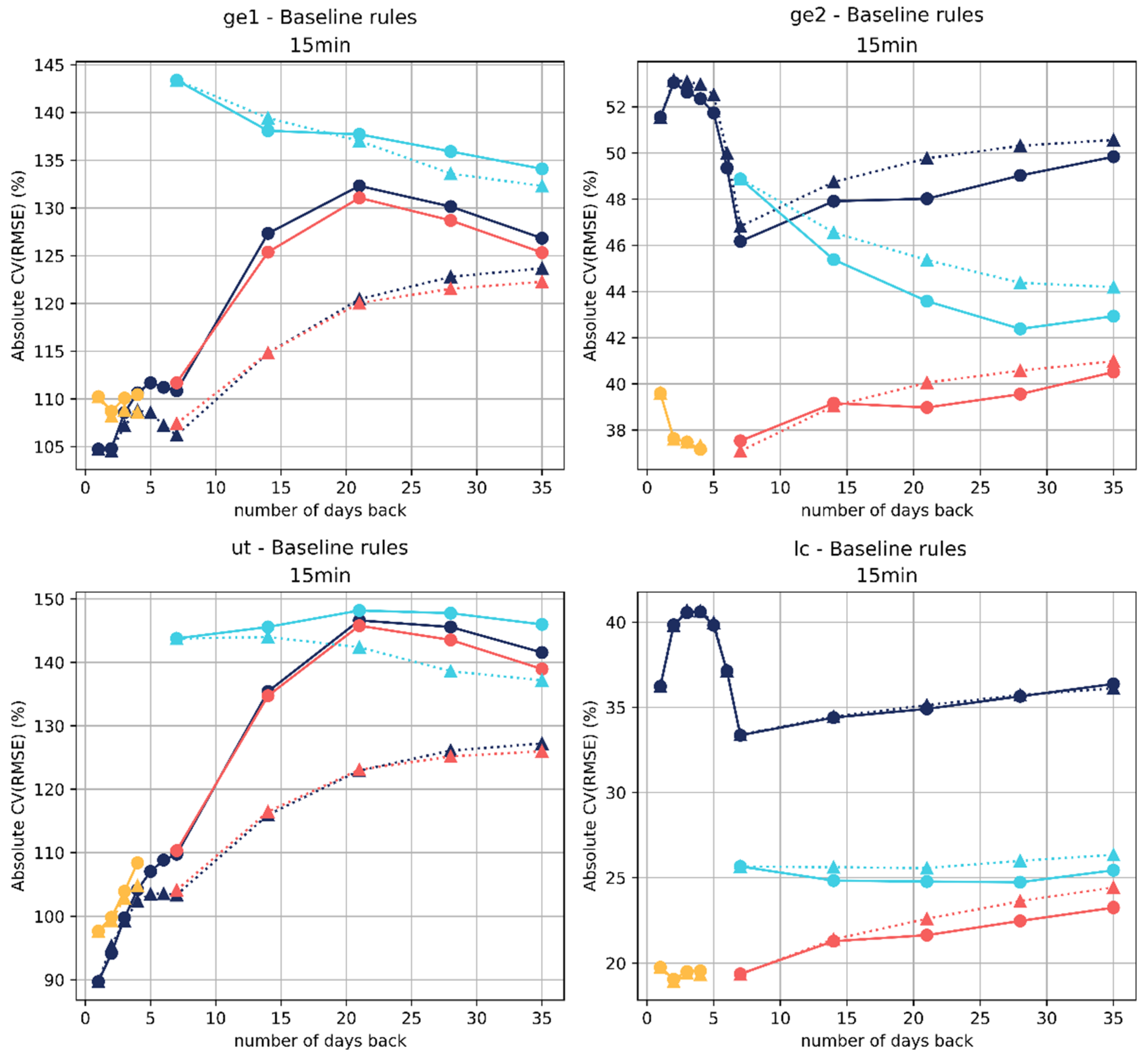
6.1. Baseline Rule Results
The following graphs contain the results of the application of the proposed baseline rules over the five power variables (see
Figure 6). On the
x-axis, the number of days back expresses the value of the hyperparameter (
n), while the
y-axis shows the absolute value of the
CV(
RMSE). The colored circular points (connected by continuous lines) correspond to the strict application of the rules, while the triangles (connected by dotted lines) are obtained from the non-strict application.
In the cases of ge1, due to its negative average value, the values of CV(RMSE) are negative. For this reason, the axes of the graphs show the absolute value of this indicator. It must be remembered that the best forecast corresponds to the lowest absolute values (the nearer to zero, the better).
It can be noted that the ge2 and lc variables show behaviors that are strongly dependent on the type of day (weekday and weekend), with the rules of type baseline_cnb (“const_num_back”) and baseline_bw (“basic_weekend”) being the best.
For ge1 and ut, the best rule is baseline_s (“simple”), as they show behaviors that are less related to the type of day. This is probably because the need for hot water (partially produced by microturbines) does not change substantially from weekdays to weekends (as many students live on campus).
Finally, pv is best forecasted using the baseline_s rule, which was expected because solar irradiation is independent of the type of day.
These results show how testing multiple types of baselines provides information about the behaviors of the variables, while addressing which type of days are the best indicators of each of these variables. Particularly, in the case of the variable ge1, whose behavior could at first be difficult to guess without a previous analysis, it was found that this variable is strongly dependent on the most recent previous days.
6.2. Machine Learning Results
The results of the RFR and MLPR models for all the different datasets that are described in
Table 2 are presented in
Figure 7. To simplify the representation of such a number of different datasets, the
x-axis groups them by the tag “dataset type”, as shown in the same table.
To avoid the presence of negative metric values, the y-axis represents the absolute value of the CV(RMSE). Therefore, the best model is the one with the minimum value.
Each of the points in the graph represents the error for a give dataset, while the red hyphens indicate the model with the minimum error value (i.e., the best model for each of the dataset types). As defined at the start of the present section, the variables ge1, ge2 and ut also include datasets with external baseline information (the expected load of the campus, i.e., lc). The variables lc and pv do not include any “EXBL” dataset, as this is not considered to be of interest.
For the RFR models, these results indicate that the dataset types “Db”, “Db + EXBL”, “DbWa” and “DbWa + EXBL” are usually the best for all variables. The two exceptions are pv, which is better forecasted by the dataset types “DbWa” and “BlWa”, and lc, whose best model for 15-min aggregations is obtained with the dataset “CaIn”.
For the MLPR models, the dataset types “Bl” and “BlWa” also obtain good performances for the variables ge2 and lc.
The comparison between the RFR and MLPR techniques for the five forecasted variables shows that the errors of the MLPR models are less than those of the RFR models for almost all variables (ge1, ge2, ut and lc), except for pv, which is better forecasted using the RFR models.
6.3. Comparison and Discussion
Once the results are obtained, the different models for each objective variable can be compared. This comparison is reported in
Table 5, which gives the
CV(
RMSE) value for the best model according to each variable, aggregation, and dataset type. To simplify the visualization of the results, the category “XX+EXBL” (the datasets that include external baseline information, as shown in
Table 5) is not detailed for each type of baseline rule, and only the model with the best indicator value is kept. Some reference models are also included, such as
baseline_s1 (previous day) and
baseline_s7 (mean of the seven previous days). The
baseline_s1 method is finally the one chosen as a reference method, as here it is considered analogous to the naïve method.
Moreover, the percentage of improvement (13) is calculated in a way similar to that reported in [
36] (with
baseline_s1 as the reference method), and the
CV(
RMSE) for the reference model and the proposed model are shown.
These results can be seen in
Table 6. The
CV(
RMSE),
RMSE and
nRMSE indicators for the best models are given. Specifically, the
nRMSE values are calculated considering the magnitudes that are included in
Figure 5.
As previously indicated, the table of improvement (
Table 6) uses
baseline_s1 as reference. However, it can be appreciated that this table is directly obtained from the numbers in
Table 5 of the results, so it is possible to calculate the relative improvements considering any other model from those included in the table applying expression (13).
Table 5 shows some interesting data about the behaviors of the evaluated models and input dataset types.
First, it can be observed that the models obtained using the RFR and MLPR are better than the best baseline models. This is expected, as according to the reviewed literature, these machine learning models usually achieve good results in the current field of study. However, it should not be forgotten that baseline models are still useful in some scenarios. They are very easy to calculate, give information about tendencies and are very clear in their behavior. Moreover, they are suitable for application in the auditory process in flexibility agreements, as a customer could be more disposed to accept one of these baseline rules than trained models, as they are RFRs and MLPRs.
Second, it is interesting to note that the use of sets that include external baselines (EXBLs) yield the best results for ge1, ge2 and ut. This fact can be explained considering that in the campus (ge2), the zone under the direct control of the EMS is precisely the microgrid (ge1) where the microturbines (ut) are installed. It is therefore logical that ge1, ge2 and ut achieve good performance when they are modeled considering the load of the campus (lc), as the EMS estimates it to manage the microgrid.
Regarding the forecasting of the load of the campus (lc variable), the datasets that include information from previous days and weather predictions for these days (dataset types “DbWa” and “BlWa”) yield the best results under the MLPR.
In the case of photovoltaic generation (pv variable), the results show that the inclusion of previous day measurements together with weather information (dataset types “DbWa” and “BlWa”) improves the modeling results. The RFR outperforms the MLPR for this variable.
The proposed models achieve accuracy improvements of up to 62% and a mean of 37% (average improvement value across the five variables and the two aggregations evaluated) over that of the reference model, which is
baseline_s1 (see
Table 6).
Finally, as an example, some illustrative comparisons between the actual data, the best baseline and the best model are shown in
Figure 8 for each of the five variables. The
CV(
RMSE) for each of the individual days is calculated for both the baseline and the best model.
It can be appreciated how the error of the baseline is usually greater than the error of the best model, with the only exception in the given examples being day number two of
Figure 8b. On this day, it can be appreciated how the best baseline model occasionally achieved a better result than the best model. However, these kinds of occurrences are expectable in the environment under study. The consumption and generation of the campus have low levels of aggregation, which produce behaviors that are difficult to predict. For this reason, on some specific days it may happen that the best selected model is outperformed by another one, which occurred on the indicated day. Despite these infrequent events, the
CV(
RMSE) (which should be taken as criterion for model selection) show from a global point of view the goodness of each model, as seen in
Table 5 and
Table 6.
7. Conclusions
As previously mentioned, forecasting is an essential tool for energy management. Many approaches apply online training, which can increase the daily computational cost (as the system must perform tasks related to updating the model daily) and does not usually involve tests with many different dataset types. Therefore, this paper presents a methodology for power variable forecasting that provides multiple combinations of information inputs and techniques without necessarily requiring online training. Therefore, model updating can be performed every few days or even every few weeks, when the inclusion of newly available historical data is desired to retrain the models. This characteristic permits a reduction of the daily computational cost incurred by the proposed framework according to current needs.
The proposed methodology provides recommendations on how to perform the analysis, which indicators can be used, and how to select the best indicators for the case under study. Specifically, it was applied to a university campus in Italy and used for the prediction of five different power variables.
Remarkably, in the proposed methodology, it is important not only to identify the best obtained model, but also to retain the information of the best model for each type of input information required. This approach makes it possible to use another model for which the system has the required inputs if for a certain day a portion of the information is missing (e.g., the weather forecast is not received). In this way, the feasibility and robustness of the system is increased, lowering the probability of failure during the forecasting process.
This methodology can be used by all the actors involved in flexibility services and/or the energy management of microgrids, i.e., DSOs, aggregators, and customers.
The applied methods include the definition of rule-based baselines, which perform forecasts using the measurements of the previous days obtained under different criteria and machine learning techniques (random forests and neural networks). Moreover, the proposed baselines are included as inputs of machine learning methods, which has been shown to improve the quality of the forecasting.
Notably, the types of datasets that can be created depend on the available information, such as the mentioned baselines, weather data, calendar information, and other data of interest (such as occupancy in cases regarding certain types of buildings).
Moreover, the forecasting horizon can also change depending on the application. In the present case study, the prediction horizon is one day, but the same models could be trained and tested using other horizons. The only requirement is to adapt the input datasets with the information that is available in the considered horizons.
The presented case study shows that an MLPR outperforms an RFR for the majority of the variables (except for the forecasting of the PV generation, pv). Moreover, the inclusion of external baseline (EXBL) information from the campus load (lc) yields a forecast improvement over those of the models in which EXBLs are not included.
From a global point of view, the presented experiments show that the proposed models achieve an accuracy improvement of up to 62% over that of the reference model.


 ,
, 


