Monitoring Total Suspended Sediment Concentration in Spatiotemporal Domain over Teluk Lipat Utilizing Landsat 8 (OLI)

Abstract

Total suspended sediment (TSS) is a water quality parameter that is used to understand sediment transport, aquatic ecosystem health, and engineering problems. The majority of TSS in water bodies is due to natural and human factors such as brought by river runoff, coastal erosion, dredging activities, and waves. It is an important parameter that should be monitored periodically, particularly over the dynamic coastal region. This study aims to monitor spatiotemporal TSS concentration over Teluk Lipat, Malaysia. To date, there are two commonly used methods to monitor TSS concentration over wide water regions. Firstly, field sampling is known very expensive and time-consuming method. Secondly, the remote sensing technology that can monitor spatiotemporal TSS concentration freely. Although remote sensing technology could overcome these problems, universal empirical or semiempirical algorithms are still not available. Most of the developed algorithms are on a regional basis. To measure TSS concentration over the different regions, a new regional algorithm needs to develop. To do so, two field trip was conducted in the study area concurrent with the passing of Landsat 8. A total of 30 field samples were collected from 30 sampling points during the first field trip and 30 samples from 30 samplings from the second field trip. The samples were then analyzed using an established method to develop the TSS algorithm. The data obtained from the first field trip were then used to develop a regional TSS algorithm using the regression analysis technique. The developed algorithm was then validated by using data obtained from the second field trip. The results demonstrated that TSS in the study area is highly correlated with three Landsat 8 bands, namely green, near-infrared (NIR), and short-wavelength (SWIR) bands, with R² = 0.79. The TSS map is constructed using the algorithm. Analyses of the image suggest that the highest TSSs are mainly observed along the coastal line and over the river mouth. It suggested that the main contributing factors over the study area are river runoff and wave splash.

1. Introduction

Total suspended sediment (TSS) is a water quality parameter that can be used to understand sediment transport, aquatic ecosystem health and engineering problems [1]. The changes in suspended sediment concentrations in the time and space domains are generally related to human and natural factors. Human factors consist of, for example, sand dredging activities, sea reclamation, shipping activities, construction, mining, and other human activities. Meanwhile, natural factors include rainfall rates, rising temperatures, winds, high waves, and all activities related to climate change. An excessively high total suspended sediments concentration will inhibit the penetration of light into water and disrupt photosynthesis [2], reduce the underwater vertical transmittance and phytoplankton productivity [2], affect the water columns and benthic processes [3], affect the nutrient dynamics [4] and pollutant movement [5,6]. Furthermore, an update of the total suspended sediments data is necessary to evaluate operational policies and provide technical guidance to the public, government, and private sectors in the utilization of coastal regions regarding environmental changes. Then, thorough studies should be done in any location directly exposed to the natural and human-induced suspended sediment.

Teluk Lipat, Malaysia, is located on the east coast of the Malaysian peninsular. This area is directly exposed to at least four suspended sediment-induced agents, such as river runoff, dredging activities and reclamation work. During the northeast monsoon season, it is also directly prone to high waves that commonly cause coastal erosion. Since Teluk Lipat is a human settlement with recreational and fishing locations for coastal anglers, it is very important to periodically monitor the spatiotemporal sediment concentration over this area. However, to date, there are no TSS data because there have been no relevant studies conducted in this location. It is well known that remote sensing sensors are widely used to monitor TSS concentrations all over the globe. The advantage of remote sensing technology is its ability to provide a historical dataset that can be used to track past events over a selected location. The remote sensing technique utilized an algorithm that was developed to measure TSS concentration over a selected region. To date, many TSS algorithms have been developed using numerous remote sensing methods, but the universal empirical or semiempirical algorithms are still unavailable [7,8,9,10,11,12,13]. In order to monitor the TSS concentration in space and time domain over this study area, an algorithm needs to be developed.

Recently, two methods have been used to monitor TSS concentration over a wide water region. The first is field sampling, which is known to be a very expensive and time-consuming method. In this procedure, water samples are collected and, after that, sifted to extricate total suspended sediment. The sifted material is, at that point, dried, weighed, and isolated by sample value to get the total suspended sediment. This strategy gives exact and point-based estimation; in any case, spatial varieties are occasionally captured, and temporal resolution is frequently limited [3,4,5]. The second uses remote sensing technology that can monitor spatiotemporal TSS concentration for free. In this technique, researchers use a few wavelengths and then relate them to the field measured TSS to develop a TSS algorithm. The utilization of remote sensing technology can diminish costs and increase spare time [6]. To date, many algorithms have been developed using various remote sensing sensors, such as MODIS, SeaWiFS, MERIS and Landsat [14]. In this study, because Landsat 8 (OLI) with a medium spatial resolution (30 m), 185 km swath, 16-day revisit time and can be obtained for free, it was considered suitable for this study area [15].

Generally, there are two distinct approaches that could be utilized to obtained water quality parameters such as TSS and Chll-a utilizing remote sensing techniques. These two approaches are empirical or semiempirical and analytical or semi-analytical methods [16,17]. Empirical or semi-empirical methods apply simple or multiple regression between measured water quality parameters and remote sensing reflectance of certain wavelengths to obtain estimated water quality parameters. The disadvantage of this method is that it is regional in nature and quite costly, particularly during field sampling procedure implementations. Meanwhile, the simplicity and rapidity of the data processing with sufficient accuracy are their main advantages [13,18]. The second approach is analytical or semi-analytical. This method incorporates spectral optimization approaches and is based on solutions to the radiative transfer equations [18]. The inversion of the radiative transfer equations is mainly based on the neural network approach, utilizing a large database of radiative transfer simulations such as the Case-2 Regional/Coast Colour (C2RCC) algorithm [19], and by using a windows-based program for modeling and analyzing optical in situ measurements in aquatic environments, such as the Water Color Simulator (WASI) [20,21]. In general, the advantages of this method are that the algorithms can be applied to the different water bodies, and the field sampling data are not required to develop the algorithm. However, the effectiveness of this kind of algorithm relies on the accuracy of the selected spectral models for the absorption coefficients of individual constituents that are present in the water; furthermore, this is a time-consuming process [18]. In general, C2RCC only works well in optically deep water, whereas water constituents such as CDOM and sediment are neglected and WASI requires more experience and supervision in defining the initial values of the parameters [21]. With the intention being to regionally monitor TSS with low cost, simple and rapid data processing, and with a sufficiently accurate empirical method, this method will be utilized in this study.

Theoretically, a single band could be used to develop the robust and sensitive TSS algorithm; if an appropriate band is chosen [3,22,23], successfully developed robust linear algorithm between TSS and red wavelength (0.62–0.67 μm) of the MODIS Terra sensor have been demonstrated over the Gulf of Mexico. However, the developed algorithm is easy to saturate when the TSS increases significantly [24]. Due to the complexity of the water body, such as the color and size of the particles, the use of more than one wavelength is more practical [22,23,25] and less sensitive to backscatter variability [26]. Recently, many researchers have developed robust and sensitive TSS algorithms by utilizing several remote sensing bands ranging from blue to the near-infrared spectrum of lights over different regional areas. Since the late 1970s, the marvel of the total suspended sediment incrementally increasing with the brilliant vitality developing from the surface waters within the visible and near-infrared (NIR) districts of the electromagnetic range has been noted [27].

Many researchers are as of now fascinated by estimating the total suspended sediment concentration by utilizing remote sensing technology. To realize this objective, field and remote sensing information must be utilized. In common, researchers calibrate remote sensing information using field information to create an algorithm. Most researchers have proposed a relationship between reflected solar radiance measured by satellite-based rebellious and field-measured total suspended sediments inside a wide range of inland and coastal waters. In previous studies, total suspended sediment remote sensing models were used by previous researchers [28,29,30,31]. However, the developed algorithms are highly regionally dependent. It is a drawback that the developed algorithm can only be applied over the study area and cannot be used in other regions. This is due to the differences in water constituents, such as sediment color, size shape and even concentration, that could influence light absorption, scattering and reflectance. That is why regional TSS algorithms must be developed.

Table 1. Review of previous TSS algorithms. For TM 4 and TM 5, the wavelength of B1,B2,B3 and B4 are 0.45–0.52, 0.52–0.60, 0.63–0.69, 0.76–0.90 µm, respectively. For Landsat 8, the wavelength for B2,B3,B4 and B8 are 0.45–0.51, 0.53–0.59, 0.64–0.67, 0.50–0.68µm, respectively. For MSI (MultiSpectral Instrument), the wavelength for B5 is 704.5 nm. For OCM-2, the wavelength for B5 and B6 are 546–566 and 610–630 nm, respectively. For MODIS Aqua, the wavelength for B1 is 620–670µm. For SPOT, the wavelengths for B2 and B4 are 0.61–0.68, 1.58–1.75 µm.

Sensor	Bands	TSS Algorithm	Study Area	References
TM 5	1, 2, 3, 4	TSS = 361.89 Rrs(0.69) − 1018.25 ((Rrs0.60)/Rrs(0.69)) − 1919.21((Rrs(0.52)/(Rrs(0.69)) − 26.15(Rrs(0.69)/Rrs(0.90)) − 182.90 Rrs(0.52) + 28855.76	Florida USA	[23]
OLI 8	3, 4	log10 (TSM) = 1.291 + 63.85 Rrs(0.67) − 50.46 Rrs(0.59)	Zhuhai-Macau Bridge Region, Hong Kong	[38]
TM 5	2, 3	ln(SSC) = (4.38 ((Rrs(0.69)/Rrs(0.60))) − 0.75	Araguaia River–Brazil	[1]
MSI	5	TSM = 0.7198 exp[329.73 Rrs(704.5)]	The Pertusillo Lake Case Study (Italy)	[40]
OLI 8	3, 4	TSS = 172.19 ln2[Rrs(0.59)/Rrs(0.67)] − 190.809 ln[Rrs(0.59)/Rrs(0.67)] + 61.6	Inland Reservoir, South China	[37]
OCM-2	5, 6	TSS = 5846.1((Rrs(566)/Rrs(630)) − 516.82	West Bengal	[36]
OLI	2, 3	log TSS = 1.5212[log(Rrs(0.51)/log(Rrs(0.59)] − 0.3698	Indonesia	[29]
OLI	2, 3, 8	TSS = −191.02 Rrs(0.51) + 36.8 Rrs(0.59) + 172:66 Rrs(0.68) + 4.57	Xin’anjiang Reservoir	[31]
TM 4	4	TSS = 229,457.695 Rrs(0.90)2 + 146.462 Rrs(0.90) + 5.701	Bohai Gulf	[32]
TM 5	2, 3	log TSS = 6.2244 (Rrs(0.60) + Rrs(0.90)/[Rrs(0.60) * Rrs(0.69)] + 0:892	Yangtze estuary	[35]
Modis Aqua	1	TSM = −1.91 (1140.25)Rrs(670)	Northern Gulf of Mexico	[3]
SPOT	2, 4	TSS = 29.022 exp 0.0335((Rrs(1.75)/Rrs(0.68))	Gironde estuaries	[28]
TM 5	1, 2	TSS = 16.826 − 5.2369 ((Rrs(0.52)/Rrs(0.60))	Moroton Bay	[30]
TM5	1, 2	ln TSS = 2.71 ((Rrs(0.52)/Rrs(0.60))2 − 9:21 ((Rrs(0.52)/Rrs(0.60)) − 8.45	Enid Reservoir in north-central Mississippi	[34]
TM 5	1, 3	TSS = 0.0167 exp[12.3 (Rrs(0.69)/Rrs(0.52)]	Embayment of Lake Michigan	[33]

shows examples of a TSS algorithm that was developed by using various remote sensing sensors and bands around the globe. The number of bands used varies from single-band [3,32], two-band [28,30,33,34] and [1,29,35,36,37] and [38], three-band [39] to four-band algorithms [23]. Recently, it was found that the difference in water constituents and seasonal dependence does not solely depend on geographical regions [23].

The aim of this study was to monitor the spatial and temporal TSS concentration over Teluk Lipat, Malaysia. The remote sensing technique was used in this study. To fulfil the aim, three objectives were set up. The first objective was to develop and validate the regional TSS algorithm utilizing the Landsat 8 (OLI) dataset. The second objective was to develop the TSS concentration map of the study area. The third objective was to analyze and investigate the TSS concentration in the space and time domains. To achieve the above-mentioned objective, two field trips were conducted in the study area. The water sample was then processed in the lab to obtain the measured TSS. The relation between the measured TSS and the Landsat surface reflectance was determined by using a regression technique. The algorithm was developed empirically by using three Landsat 8 (OLI) bands: band 3 (Green, λ = 0.53–0.59 µm), band 5 (near Infrared, λ = 0.85–0.88 µm) and band 6 (short-wave infrared, λ = 1.57–1.65 µm). A TSS map was then created by applying the developed algorithm. The map was then analyzed to extract the required information. Since the algorithm was only validated with the data that was acquired over the study area, the application of the developed algorithm was limited to Teluk Lipat, Malaysia.

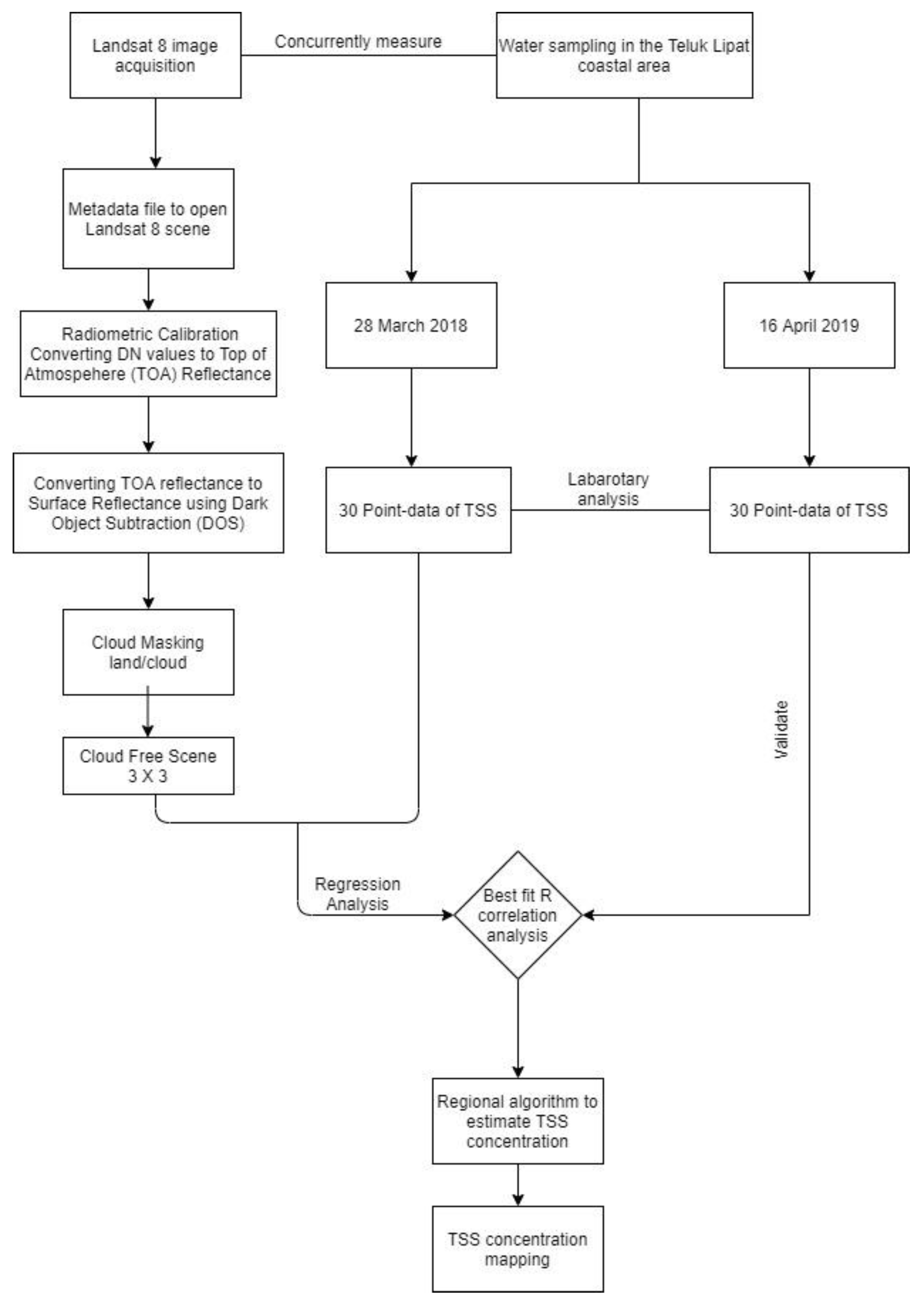
2. Materials and Methods

2.1. Study Region

Teluk Lipat, as shown in Figure 1, is located in Terengganu, Malaysia. In 2011, severe erosion occurred along this beach due to a high tidal surge phenomenon. The tidal wave ravaged the wall road and crumpled the trees along the coastline. This beach extends approximately 13 km to Kuala Dungun from Bukit Bauk, which is in the south. A university, a school and residential housing are located along this coastline. The study region covers the latitude range of 4°39′5.12″–4°48′21.74″ north and the longitude range of 103°23′28.33″–103°30′12.11″ south.

2.2. Data Sampling and Analysis

Two field trips were conducted in the study area. The first and second field trips were conducted on 28 March 2018, and 16 April 2019, respectively. During the first campaign, 30 in situ samples were collected from 30 sampling points. Meanwhile, 30 water samples were obtained from the second field trip collected from 30 stations. The distance between each sampling point is 1 km. Both field trips were conducted concurrently with the passing of Landsat 8 over the study area. Sample testing was conducted 2 h before and 2 h after the passing of Landsat 8 to maintain a strategic distance from the impact of TSS changeability related to tides and nearby streams [5,41]. Water samples, approximately 1.5 L, were collected inside a profundity of 1 m, and sample concentrations were measured employing a pondering method [42,43]. The TSS concentration was calculated based on the difference of a filter paper before (without TSS residue) and after (with TSS residue) the filter was dried. A Sartoris MGF glass fiber filter (47 mm diameter) was used. In this study, a well-mixed sample was filtered through a weighed standard glass-fiber filter, and the TSS residue was retained on the filter. Before removing the filter from the filtration apparatus, 3 successive 10 mL volumes of deionized water were used to wash the filter, allowing complete drainage between washings. Then, the filter was removed and dried in an oven at 103–105 °C for 1 h and left it cool in desiccators. The cool filter paper with TSS residue was weighed using a weighing balance. The process of heating, cooling, and weighing was repeated until a constant weight was obtained or until weight change was less than 4% of the previous weighing or 0.5 mg—whichever was less. The TSS concentration in the water sample was calculated using the following formula:

$$\mathrm{TSS} \left(\mathrm{mg}/\mathrm{L}\right)=\frac{\left(\mathrm{A} -\mathrm{B}\right)}{\mathrm{Volume} \mathrm{of} \mathrm{filtered} \mathrm{sample} \left(\mathrm{L}\right)}$$

(1)

where,

• A = mass of filter + dried residue (mg),
• B = mass of filter (tare weight) (mg)

2.3. Landsat 8 Dataset

This study utilized Landsat 8 level 1 TP products. Level 1 TP is the most elevated quality of level 1 product that is reasonable for pixel-level time series analysis. The image acquired on 28 March 2018, was used for model implementation. Meanwhile, the image acquired on 16 April 2019, was elaborated for validation purposes. Images acquired on 23 November 2018, 17 September 2017, 26 June 2016, and 23 July 2020, were used to develop the TSS concentration map over the study area. These images were carefully selected to ensure minimal cloud cover. All images were downloaded from the EarthExplorer website and, after that, processed using ENVI 5.1. Atmospheric correction was executed to eliminate the effect of the atmospheric haze present in the image. A few atmospheric corrections are accessible. The DOS atmospheric method was used in this study due to its effectiveness in eliminating atmospheric hazards. This atmospheric correction method has been widely used by many researchers in order to obtain water quality parameters around the globe [3,44,45,46,47,48,49,50]. To realize this objective, radiometric calibration was performed to convert radiance, and the surface brightness was measured directly by the satellite, to the unit with less surface reflectance utilizing metadata which approximated the procurement time and sun elevation when the image was taken [50]. From that point, the DOS calculation was performed. DOS searched each band for the darkest pixel value. Expecting that dark objects do not reflect light, any esteem more prominent than zero must have come about from atmospheric scattering. Such scattering was removed by subtracting this esteem from every pixel within the band. This basic procedure is compelling for haze correction in multispectral information, but ought to not be utilized for hyperspectral information. Clouds that were shown within the image were masked utilizing Landsat 8 cloud mask product. During this process, the classification of pixel QA bands was analyzed. The pixel QA band quality conditions are expressed as a cloud confidence level. In this study, only pixels with a clear condition (no cloud), low cloud confidence (LCC) and low cloud shadow (LCS) were used in the cloud masking method [32,51,52].

2.4. Matchup

In this study, three methods were tested for matchup analysis: 1 × 1, 3 × 3 and 5 × 5-pixel windows. In the 1 × 1 pixel method, the station coordinate was directly matched to the associated pixel. To improve the interpretability and quality of the remote sensing images, radiometric correction was performed by comparing the coordinates on Landsat 8 products with the images on Google Maps. The comparison showed that the coordinates exactly matched the Google Map coordinates. The surface reflectance values of the 3 × 3 and 5 × 5-pixel methods were averaged to the pixel grid, surrounding the sampling point to diminish per-pixel noise.

2.5. Accuracy Assessment Method of Models

In order to validate the accuracy of the TSS spectral models, atmospheric correction and mapping of TSS concentrations, the most frequently used methods including the determination coefficient (R²), the RMSE and mean relative error (MRE), were also used in the study for the convenience of comparison by different readers.

$$\mathrm{RMSE} =\sqrt{\frac{{{\displaystyle \sum }}_{i=1}^{i=n}{\left(x_i-{x^{\prime }}_i\right)}^2}{n}}$$

(2)

$$\mathrm{MRE}=\frac{{{\displaystyle \sum }}_{i=1}^{i=n}\left|\frac{x_i-x{\prime }_i}{x_i}\right|}{n}\times 100\%$$

(3)

where x_i is the in-situ value, x’_i is the estimated value, i is the ith element, and n is the number of elements. Figure 2 summarized the flowchart of the data processing scheme of this study.

3. Results and Discussion

3.1. Pixel Dimension

Regression was conducted by utilizing the three windows (1 × 1, 3 × 3 or 5 × 5) to determine which one was the best for this study. The results confirmed that the 3 × 3 window achieved the best R² value compared with those of the two other windows.

Table 2. Regression analysis for different windows.

Window	Algorithm	R2
1 × 1	y = 659.26x − 468.15	0.62
3 × 3	y = 564.68x − 881.98	0.79
5 × 5	y = 557.53x − 358.4	0.77

shows the result of the application of different windows. It can be clearly seen that the lowest and highest R² values were obtained by the 1 × 1 and 3 x 3 windows, respectively. The R² value for each window is given by 0.62, 0.79 and 0.77, respectively. This result indicated that the regression coefficient decreased when the window was larger than 3 × 3. Furthermore, 3 × 3 windows instead of 1 × 1 and 5 × 5 windows have been widely used and discussed by previous researchers [34,53,54,55,56].

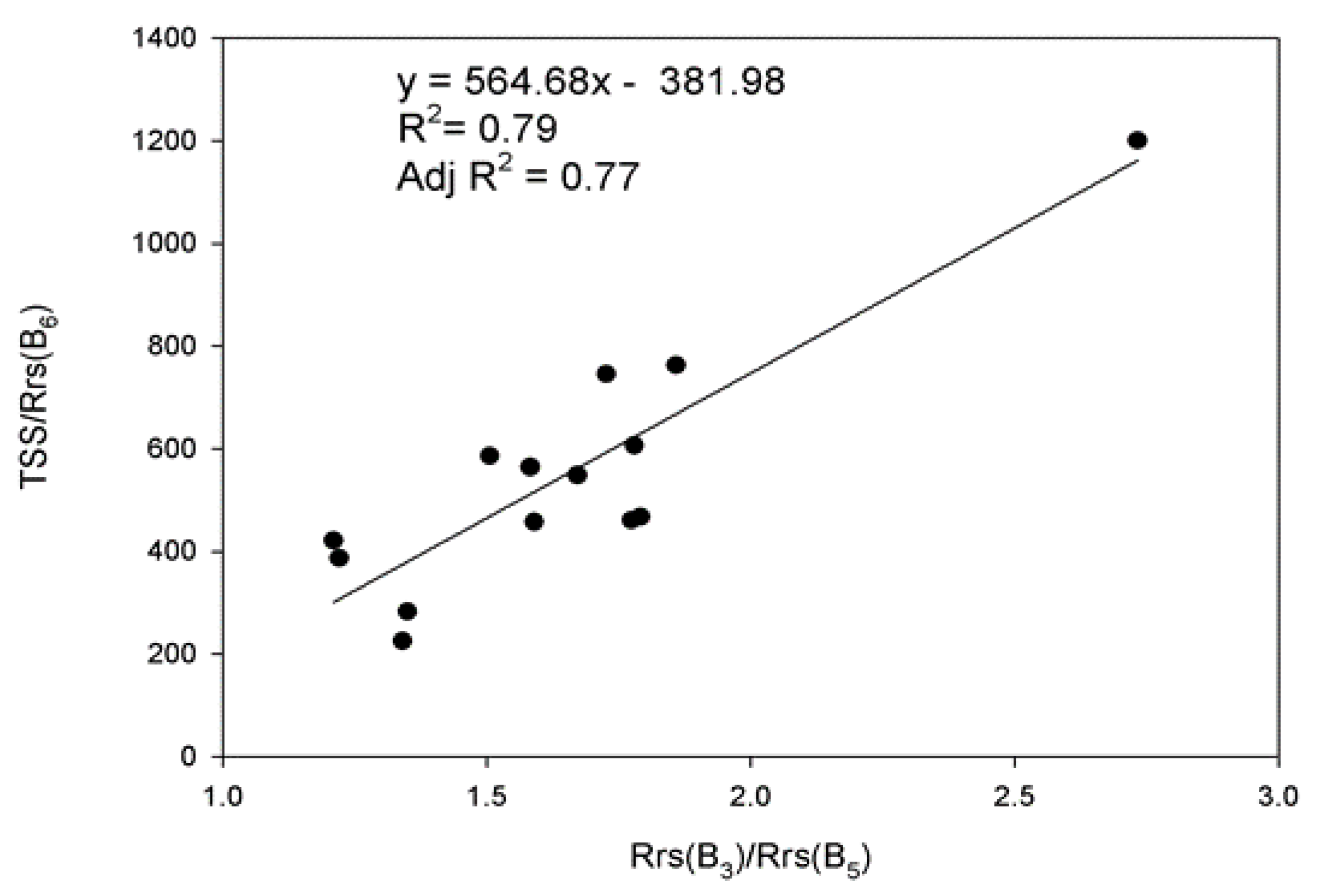
3.2. TSS Concentration Algorithm

The TSS concentration retrieval algorithm was created utilizing the regression algorithm between the in situ TSS concentration and the in situ-measured remote sensing reflectance, Rrs (λ), based on single-band, two-band, and three-band proportion reflectance combinations. The in situ TSS concentration and in situ Rrs (λ) were utilized as the dependent and independent variables, respectively. Among the few combinations, the most elevated relationship between the two variables was shown by the most elevated coefficient of determination (R²), which was chosen as the retrieval algorithm. The regression algorithm for TSS concentrations is displayed in

Table 3. Regression results of TSS against several Landsat 8 bands. B₁-B₇ represent the designated band of Landsat OLI. The wavelength for seven spectral Landsat bands (B₁–B₇) used in this study are 0.43–0.45, 0.45–0.51, 0.53–0.59, 0.64–0.67, 0.85–0.88, 1.57–1.65 and 2.11–2.29 µm, respectively.

Band	Best Fit Equation	R2
Single
B1	TSS = −114.26 Rrs(B1) + 14.859	0.0607
B2	TSS = −91.935 Rrs(B2) + 15.012	0.0505
B3	TSS = −50.83 Rrs(B3) + 13.746	0.0414
B4	TSS = −88.187 Rrs(B4) + 13.782	0.0767
B5	TSS = −74.862 Rrs(B5) + 13.626	0.0815
B6	TSS = −124.15 Rrs(B6) + 14.25	0.1061
B7	TSS = −156.87 Rrs(B7) + 14.122	0.1092
Two band
B6/B7	TSS = 15.55 Rrs(B6/B7) − 9.1884	0.0605
B6/B5	TSS = 0.2873 Rrs(B6/B5) + 11.304	0.0001
B3/B4	TSS = 4.131 Rrs(B3/B4) + 4.3269	0.1131
Three band
TSS/B1 vs. B2/B3	TSS= Rrs (B1)[−2502.5 Rrs(B2/B3) + 2330]	0.2819
TSS/B6 vs. B4/B5	TSS= Rrs(B4)[1426(B5/B6) − 745.37]	0.3707
TSS/B6 vs. B3/B5	TSS = Rrs (B6)[564.68 Rrs(B3/B5) − 381.98]	0.7900
TSS/B7 vs. B3/B4	TSS = Rrs (B7)[566.47 Rrs(B3/B4)2 – 635.62 Rrs(B3/B4) + 116.79]	0.7619
TSS/B6 vs. B3/B4	TSS = Rrs (B6)[399.41 Rrs(B3/B4)2 – 439.7 Rrs(B3/B4) + 97.191]	0.7570

.

As shown by Table 3, the highest R² value for single-band regression obtained by SWIR (short-wave infrared) wavelength with the value is 0.1092. Meanwhile, the lowest was obtained by the blue band, with R² = 0.0505. Meanwhile, the result of two band shows that the lowest R² obtained by the ratio of SWIR/NIR bands with the value is 0.0001 and the highest value obtained by ratio green to red bands with the R² value is 0.1131. The above result shows that the regression between TSS/Rrs(B₆) in Teluk Lipat waters was strongly associated with Rrs(B₃)/Rrs(B₅), with the highest coefficients of determination R² = 0.7900 with the standard error of estimate (SEE) being 119.804.

Figure 3 shows the plot of TSS over band 6 against Rrs(B₃)/Rrs(B₅). The R² and adjR² for this plot are given by 0.79 and 0.77, respectively. As compared to the algorithm developed by [32], this result fully utilized the different sensitivities of the green, NIR and SWIR bands to TSS concentrations, as proven by many previous studies [25,57]. Furthermore, the effectiveness of NIR wavelengths to assess TSSs is well documented [58]. Thus, these band combinations were selected for estimating TSS in Teluk Lipat. The equation is given by

$$\mathrm{TSS}=x_1\left[a\left(\frac{x_2}{x_3}\right) - b\right]$$

(4)

where,

• x₁ = Rrs(B₆)
• x₂ = Rrs(B₃)
• x₃ = Rrs(B₅)
• a = 564.68, b = 381.98

3.3. Validation of the TSS Concentration Model

To predict the TSS concentration using the Landsat 8 OLI data, the atmospherically corrected band ratio of the validation points coordinates obtained from the second field trip on 16 April 2019 were used. Only seven points from the second campaign were used for validation. This is because 27 sampling points were covered by clouds and failed the cloud masking process. From the previous researcher, the number of points for validation is considered acceptable if it is comparable to the test point data [59,60,61]. The reflectance ratios of the validation points were given as the input to the prediction model Equation (4) and the model output was considered as the predicted TSS concentration values of the validation points (satellite-derived). The regression model statistics between laboratory-derived in situ TSS concentration value and model-fitted TSS concentration value of the validation points revealed a strong correlation R² = 0.8406 with an RMSE of 1.50 mg/L and MRE = 9.14%. The testing of the accuracy level of TSS concentrations from satellite data within situ data is presented in Figure 3. The root means square error (RMSE) has been used as a standard statistical metric to measure model performance in meteorology, air quality, and climate research studies [62,63,64]. The mean relative error (MRE) is another useful measure widely used in model evaluations. While they have both been used to assess model performance for many years, there is no consensus on the most appropriate metric for model errors. In the field of remote sensing, many present the RMSE as a standard metric for model errors [62,63,64], while a few others choose to avoid the RMSE and present only the MRE, citing the ambiguity of the RMSE claimed by [65,66,67,68,69]. While the MRE gives the same weight to all errors, the RMSE penalizes variance as it gives errors with larger absolute values more weight than errors with smaller absolute values. The calculation results of the accuracy test between the measurement of in situ data with the prediction of the distribution of TSS are distinguished by RMSE and MRE. Based on Figure 3, the root mean square error in the statistical test was 1.50 mg/L. The size of the error is shown based on the difference between the value of the estimated data and in situ data. The greater the value of RMSE means that the results of the estimation model produced were increasingly inappropriate when compared to in situ. In this study, the RMSE value was smaller than the MRE value shown in Figure 4, which indicated that this model was accurate. There is no size or limit for determining how big the RMSE value is, but the condition is that the RMSE value should not be greater than the MRE value. The mean relative error (MRE) value of 9.14% indicated the error rate expressed in percent (%). Error values (MRE) below 30% could be used as proof of the validity of the model [70].

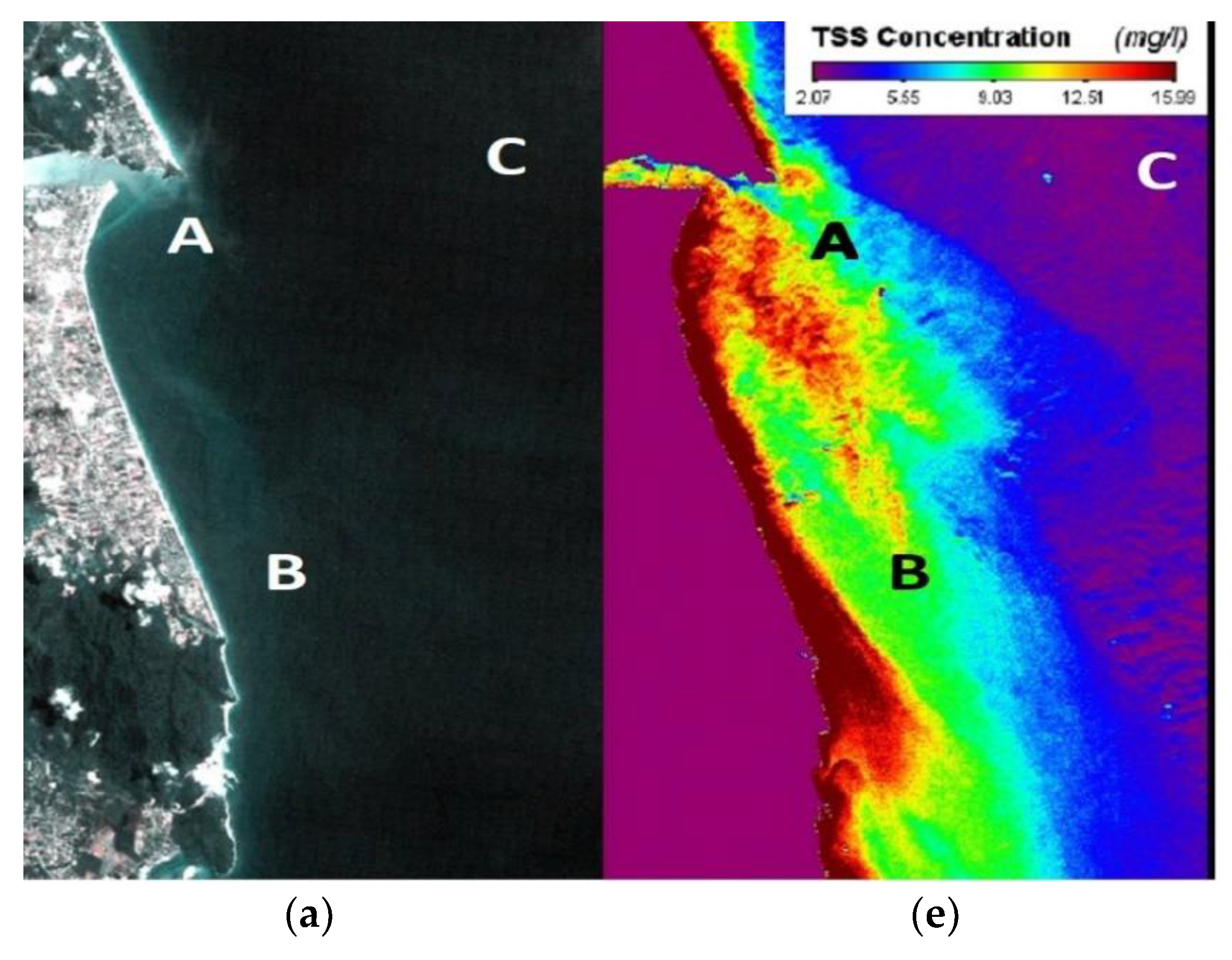
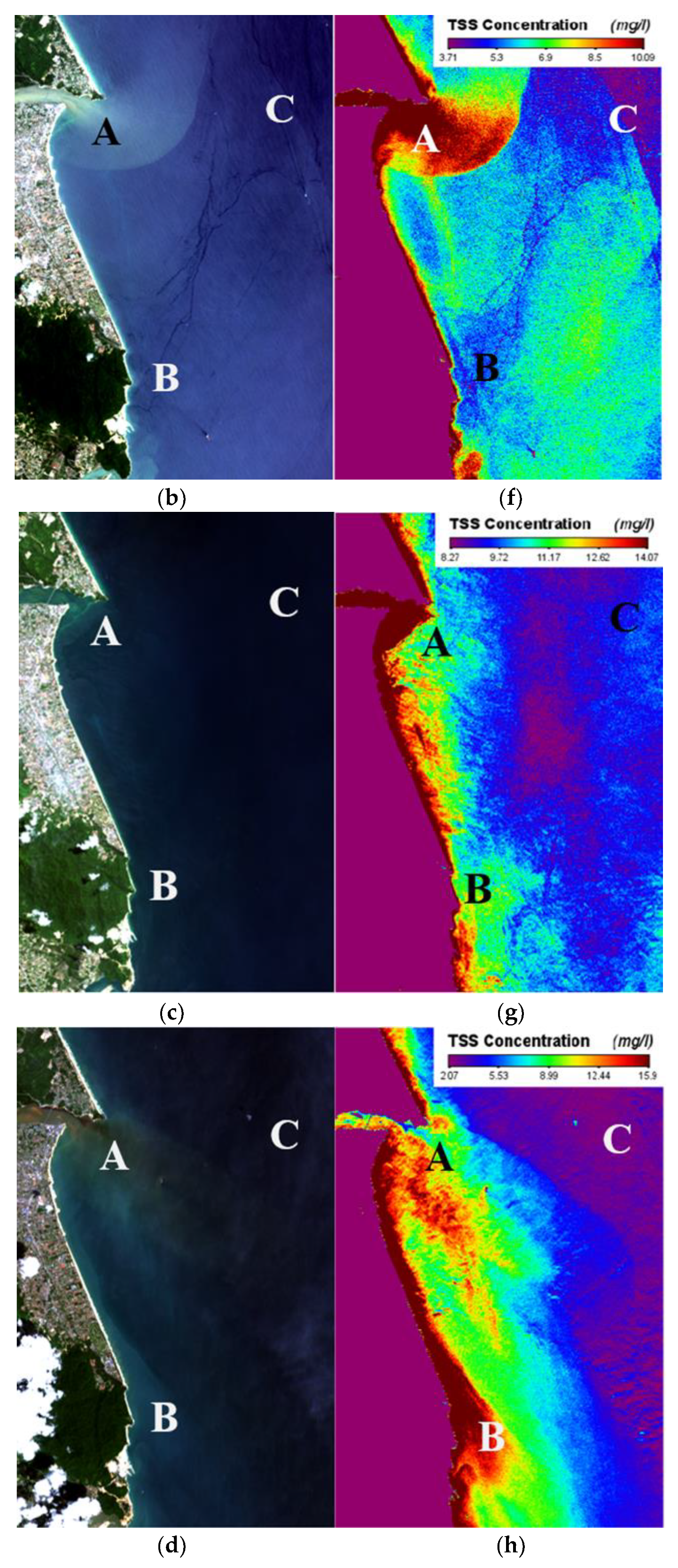
3.4. TSS Concentration Mapping

The above-developed algorithm was tested over the study for the number of Landsat datasets. The images were carefully selected and processed to produce the TSS map. Figure 5a–d show the Landsat true color images (Red: Band 4, Green: Band 3, Blue: Band 2) acquired. Meanwhile, Figure 5e–f shows the TSS concentration map derived from Landsat dataset utilizing the above-mentioned algorithm.

Figure 5a,e show a Landsat true color image and TSS map constructed over the study area for 23 November 2018. Points A, B, and C represent river estuary, coastal, and open water areas. It can be clearly seen that the highest TSS is observed along the coastal line, with the highest value being 15.99 mg/L, covers an area of 9.43 km². The lowest TSS concentration is observed at point C, as represented by purple. The moderate TSS concentration, the yellowish color in Figure 5e, covers an area of about 23.11 km².

Figure 5b shows true color images over the study area for the date of 17 September 2017. It can clearly be seen that the sediment plume at the river mouth appears to be moving north. Meanwhile, Figure 5f shows the TSS concentration produced from the developed algorithm for the abovementioned date. The range of TSS concentrations for this date is 0 to 10.09 mg/L. The sediment plume shown in the true color image was successfully mapped. The concentration of this plume is between 8.06 and 10.09 mg/L, as shown in the legend, and covers an area of 7.00 km². The same sediment concentration was observed along the coastal line. The highest TSS concentration is at point A, located at the river mouth. The low TSS observed at points B and C are represented by the bluish and purple color.

Figure 5c,g are the images obtained over the study area on 26 June 2016. In Figure 5g, the variation of TSS concentration along the coastal line can be clearly seen. The highest TSS concentration is observed at point B and along the coastal line. At this point, the highest TSS concentration is about 15.90 mg/L. At point A, a moderate TSS concentration can be seen, as represented by the yellow and greenish color. Far from the coastal line as at point B, the TSS concentration decreased gradually. For this date, the TSS concentration varies from 2.07 to 15.90 mg/L.

Figure 5d shows the RGB image for the date of 23 July 2020. The highest TSS concentration is 14.07 and covers an area along the coastal line, particularly over the river estuary, point A. A moderate TSS concentration was observed at points B and C. The TSS value at points C and B is 9.00 and 11.00 mg/L, respectively, as shown in Figure 5h. Visual observation shows that the sediment appeal drifted to the south.

4. Conclusions

The main intention of this study monitors spatiotemporal TSS concentration over Teluk Lipat Malaysia utilizing Landsat 8 datasets. The three earlier stated objectives were successfully achieved. In this study, the regional TSS algorithm with regression coefficient, R² = 0.79 utilizing three Landsat 8 channels (Green, NIR, and SWIR), was successfully developed and validated. The regression statistics model between laboratory-derived in situ value and model-fitted TSS concentration value of the validation points revealed a strong correlation with R² = 0.8406, RMSE of 1.50 mg/L, and MRE = 9.14%. The TSS map is constructed using the developed algorithm. Analyses of the map suggested that most of the suspended sediment was distributed along the coastal line and over the river mouth. It is suggested that the TSS in this area are mostly transported by the river and induced by the wave. Others identified that the suspended, induced factors are sand dredging activities and embarkment projects. This study successfully and clearly determined the direction of sediment transport. Thus, these variables ought to be considered in future studies to make strides in the adaptiveness of the demonstrated assistance. TSS in coastal waters continuously and significantly shifts in the daytime due to water runoff, diurnal tidal periodicity, human exercises, and coming within the deficient, worldly determination of these sensors. This issue postures one of the restrictions in giving a high-accuracy strategy for checking TSS concentration in coastal ranges. Therefore, the researchers suggest that a similar study needs to be conducted in a different location for comparison. This study suggests that a similar study in Penang, Malaysia, would be useful as it is currently active in the reclamation activities and has higher effects on coastline changes, socio-economic and development issues. The basic comparison may provide a better understanding of the aptness of the assessment method of models.

References

1. Cremon, É.H.; Da Silva, A.M.S.; Montanher, O. Estimating the suspended sediment concentration from TM/Landsat-5 images for the Araguaia River—Brazil. Remote Sens. Lett. 2020, 11, 47–56. [Google Scholar] [CrossRef]
2. May, C.L.; Koseff, J.R.; Lucas, L.V.; Cloern, J.; Schoellhamer, D.H. Effects of spatial and temporal variability of turbidity on phytoplankton blooms. Mar. Ecol. Prog. Ser. 2003, 254, 111–128. [Google Scholar] [CrossRef] [Green Version]
3. Miller, R.L.; McKee, B.A. Using MODIS Terra 250 m imagery to map concentrations of total suspended matter in coastal waters. Remote Sens. Environ. 2004, 93, 259–266. [Google Scholar] [CrossRef]
4. Mayer, L.M.; Keil, R.G.; Macko, S.A.; Ruttenberg, K.C.; Aller, R.C.; Joye, S.B. Importance of suspended participates in riverine delivery of bioavailable nitrogen to coastal zones. Glob. Biogeochem. Cycles 1998, 12, 573–579. [Google Scholar] [CrossRef]
5. Vinh, P.Q.; Ha, N.T.T.; Binh, N.T.; Thang, N.N.; Oanh, L.T.; Thao, N.T.P. Developing algorithm for estimating chlorophyll-a concentration in the Thac Ba Reservoir surface water using Landsat 8 Imagery. Vietnam J. Earth Sci. 2019, 41, 10–20. [Google Scholar] [CrossRef] [Green Version]
6. Olsen, C.; Cutshall, N.; Larsen, I. Pollutant—Particle associations and dynamics in coastal marine environments: A review. Mar. Chem. 1982, 11, 501–533. [Google Scholar] [CrossRef]
7. Ma, W.-X.; Huang, T.; Zhang, Y. A multiple exp-function method for nonlinear differential equations and its application. Phys. Scr. 2010, 82, 1–12. [Google Scholar] [CrossRef]
8. Wu, W.; Zheng, H.; Xu, S.; Yang, J.; Liu, W. Trace element geochemistry of riverbed and suspended sediments in the upper Yangtze River. J. Geochem. Explor. 2013, 124, 67–78. [Google Scholar] [CrossRef]
9. Phuong, N.T.B.; Tri, V.P.D.; Duy, N.B.; Nghiem, N.C. Remote Sensing for Monitoring Surface Water Quality in the Vietnamese Mekong Delta: The Application for Estimating Chemical Oxygen Demand in River Reaches in Binh Dai, Ben Tre. Vietnam J. Earth Sci. 2017, 39, 256–268. [Google Scholar] [CrossRef] [Green Version]
10. Wang, M. Estimation of ocean contribution at the MODIS near-infrared wavelengths along the east coast of the U.S.: Two case studies. Geophys. Res. Lett. 2005, 32, 1–5. [Google Scholar] [CrossRef] [Green Version]
11. Ronghua, M.; Junwu, T.; Hongtao, D.; Delu, P. Progress in lake water color remote sensing. J. Lake Sci. 2009, 21, 143–158. [Google Scholar] [CrossRef]
12. Mountrakis, G.; Im, J.; Ogole, C. Support vector machines in remote sensing: A review. ISPRS J. Photogramm. Remote Sens. 2011, 66, 247–259. [Google Scholar] [CrossRef]
13. Wang, C.; Chen, S.; Li, D.; Wang, D.; Liu, W.; Yang, J. A Landsat-based model for retrieving total suspended solids concentration of estuaries and coasts in China. Geosci. Model Dev. 2017, 10, 4347–4365. [Google Scholar] [CrossRef] [Green Version]
14. Zheng, Z.; Li, Y.; Guo, Y.; Xu, Y.; Liu, G.; Du, C. Landsat-Based Long-Term Monitoring of Total Suspended Matter Concentration Pattern Change in the Wet Season for Dongting Lake, China. Remote Sens. 2015, 7, 13975–13999. [Google Scholar] [CrossRef] [Green Version]
15. Mukhtar, M.; Manessa, M.; Supriatna, S.; Khikmawati, L. Spatial Modeling of Potential Lobster Harvest Grounds in Palabuhanratu Bay, West Java, Indonesia. Fishes 2021, 6, 16. [Google Scholar] [CrossRef]
16. Matthews, M.W. A current review of empirical procedures of remote sensing in inland and near-coastal transitional waters. Int. J. Remote Sens. 2011, 32, 6855–6899. [Google Scholar] [CrossRef]
17. Maier, P.; Keller, S.; Hinz, S. Deep Learning with WASI Simulation Data for Estimating Chlorophyll a Concentration of Inland Water Bodies. Remote Sens. 2021, 13, 718. [Google Scholar] [CrossRef]
18. Lee, Y.K.; Ng, H.T. An empirical evaluation of knowledge sources and learning algorithms for word sense disambiguation. In Proceedings of the 2002 Conference on Empirical Methods in Natural Language Processing (EMNLP 2002), Philadelphia, PA, USA, 6–7 July 2002; pp. 41–48. [Google Scholar]
19. Brockman, G.; Cheung, V.; Pettersson, L.; Schneider, J.; Schulman, J.; Tang, J.; Zaremba, W. OpenAI Gym. 2016, pp. 1–4. Available online: http://arxiv.org/abs/1606.01540 (accessed on 10 June 2021).
20. Gege, P. The water color simulator WASI: An integrating software tool for analysis and simulation of optical in situ spectra. Comput. Geosci. 2004, 30, 523–532. [Google Scholar] [CrossRef]
21. Niroumand-Jadidi, M.; Bovolo, F.; Bruzzone, L.; Gege, P. Inter-Comparison of Methods for Chlorophyll-a Retrieval: Sentinel-2 Time-Series Analysis in Italian Lakes. Remote Sens. 2021, 13, 2381. [Google Scholar] [CrossRef]
22. Nechad, B.; Ruddick, K.; Park, Y. Calibration and validation of a generic multisensor algorithm for mapping of total suspended matter in turbid waters. Remote Sens. Environ. 2010, 114, 854–866. [Google Scholar] [CrossRef]
23. Hajigholizadeh, M.; Moncada, A.; Kent, S.; Melesse, A. Land–Lake Linkage and Remote Sensing Application in Water Quality Monitoring in Lake Okeechobee, Florida, USA. Land 2021, 10, 147. [Google Scholar] [CrossRef]
24. Balasubramanian, S.V.; Pahlevan, N.; Smith, B.; Binding, C.; Schalles, J.; Loisel, H.; Gurlin, D.; Greb, S.; Alikas, K.; Randla, M.; et al. Robust algorithm for estimating total suspended solids (TSS) in inland and nearshore coastal waters. Remote Sens. Environ. 2020, 246, 111768. [Google Scholar] [CrossRef]
25. Feng, L.; Hu, C.; Chen, X.; Song, Q. Influence of the Three Gorges Dam on total suspended matters in the Yangtze Estuary and its adjacent coastal waters: Observations from MODIS. Remote Sens. Environ. 2014, 140, 779–788. [Google Scholar] [CrossRef]
26. Di Trapani, A.; Corbari, C.; Mancini, M. Effect of the Three Gorges Dam on Total Suspended Sediments from MODIS and Landsat Satellite Data. Water 2020, 12, 3259. [Google Scholar] [CrossRef]
27. Ritchie, F.R.; Ritchie, M.J.R.; Schiebe, J.C. Remote sensing of Ss in surface water. Photogramm. Eng. Remote Sens. 1976, 42, 1539–1545. [Google Scholar]
28. Doxaran, D.; Froidefond, J.-M.; Castaing, P. Remote-sensing reflectance of turbid sediment-dominated waters. Reduction of sediment type variations and changing illumination conditions effects by use of reflectance ratios. Appl. Opt. 2003, 42, 2623–2634. [Google Scholar] [CrossRef] [PubMed]
29. Jaelani, L.M.; Limehuwey, R.; Kurniadin, N.; Pamungkas, A.; Koenhardono, E.S.; Sulisetyono, A. Estimation of Total Suspended Sediment and Chlorophyll-A Concentration from Landsat 8-Oli: The Effect of Atmospher and Retrieval Algorithm. IPTEK J. Technol. Sci. 2016, 27. [Google Scholar] [CrossRef] [Green Version]
30. Islam, S.; Sarker, J.; Yamamoto, T.; Wahab, A.; Tanaka, M. Water and sediment quality, partial mass budget and effluent N loading in coastal brackishwater shrimp farms in Bangladesh. Mar. Pollut. Bull. 2004, 48, 471–485. [Google Scholar] [CrossRef] [PubMed]
31. Zhang, Y.-B.; Zhang, Y.-L.; Zha, Y.; Shi, K.; Zhou, Y.; Wang, M.-Z. Remote sensing estimation of total suspended matter concentration in Xin’anjiang Reservoir using Landsat 8 data. Huan Jing Ke Xue Huanjing Kexue 2015, 36, 56–63. [Google Scholar]
32. Chen, S.; Han, L.; Chen, X.; Li, D.; Sun, L.; Li, Y. Estimating wide range Total Suspended Solids concentrations from MODIS 250-m imageries: An improved method. ISPRS J. Photogramm. Remote Sens. 2015, 99, 58–69. [Google Scholar] [CrossRef]
33. Lathrop, R.G.; Lillesand, T.M.; Yandell, B.S. Testing the utility of simple multi-date Thematic Mapper calibration algorithms for monitoring turbid inland waters. Remote Sens. 1991, 12, 2045–2063. [Google Scholar] [CrossRef]
34. Ritchie, J.C.; Cooper, C.M. An algorithm for estimating surface suspended sediment concentrations with landsat mss digital data. JAWRA J. Am. Water Resour. Assoc. 1991, 27, 373–379. [Google Scholar] [CrossRef]
35. Wang, G.; Dong, J.; Li, X.; Sun, H. The bacterial diversity in surface sediment from the South China Sea. Acta Oceanol. Sin. 2010, 29, 98–105. [Google Scholar] [CrossRef]
36. Pitchaikani, J.S.; Ramakrishnan, R.; Bhaskaran, P.K.; Ilangovan, D.; Rajawat, A.S. Development of Regional Algorithm to Estimate Suspended Sediment Concentration (SSC) Based on the Remotely Sensed Reflectance and Field Observations for the Hooghly Estuary and West Bengal Coastal Waters. J. Indian Soc. Remote Sens. 2018, 47, 177–183. [Google Scholar] [CrossRef]
37. Zhao, J. Remote Sensing Evaluation of Total Suspended Solids Dynamic with Markov Model: A Case Study of Inland Reservoir across Administrative Boundary in South China. Sensors 2020, 20, 6911. [Google Scholar] [CrossRef] [PubMed]
38. Liu, F.; Zhang, T.; Ye, H.; Tang, S. Using Satellite Remote Sensing to Study the Effect of Sand Excavation on the Suspended Sediment in the Hong Kong-Zhuhai-Macau Bridge Region. Water 2021, 13, 435. [Google Scholar] [CrossRef]
39. Shi, K.; Zhang, Y.; Zhu, G.; Liu, X.; Zhou, Y.; Xu, H.; Qin, B.; Liu, G.; Li, Y. Long-term remote monitoring of total suspended matter concentration in Lake Taihu using 250 m MODIS-Aqua data. Remote Sens. Environ. 2015, 164, 43–56. [Google Scholar] [CrossRef]
40. Ciancia, E.; Campanelli, A.; Lacava, T.; Palombo, A.; Pascucci, S.; Pergola, N.; Pignatti, S.; Satriano, V.; Tramutoli, V. Modeling and Multi-Temporal Characterization of Total Suspended Matter by the Combined Use of Sentinel 2-MSI and Landsat 8-OLI Data: The Pertusillo Lake Case Study (Italy). Remote Sens. 2020, 12, 2147. [Google Scholar] [CrossRef]
41. Matus-Hernández, M. Ángel; Hernández-Saavedra, N.Y.; Martínez-Rincón, R.O. Predictive performance of regression models to estimate Chlorophyll-a concentration based on Landsat imagery. PLoS ONE 2018, 13, e0205682. [Google Scholar] [CrossRef] [Green Version]
42. Binding, C.; Greenberg, T.; Bukata, R. An analysis of MODIS-derived algal and mineral turbidity in Lake Erie. J. Great Lakes Res. 2012, 38, 107–116. [Google Scholar] [CrossRef]
43. Caballero, I.; Morris, E.; Ruiz, J.; Navarro, G. Assessment of suspended solids in the Guadalquivir estuary using new DEIMOS-1 medium spatial resolution imagery. Remote Sens. Environ. 2014, 146, 148–158. [Google Scholar] [CrossRef] [Green Version]
44. Isenstein, E.M.; Kim, D.; Park, M.-H. Modeling for multi-temporal cyanobacterial bloom dominance and distributions using landsat imagery. Ecol. Inform. 2020, 59, 101119. [Google Scholar] [CrossRef]
45. Obaid, A.; Ali, K.; Abiye, T.; Adam, E. Assessing the utility of using current generation high-resolution satellites (Sentinel 2 and Landsat 8) to monitor large water supply dam in South Africa. Remote Sens. Appl. Soc. Environ. 2021, 22, 100521. [Google Scholar] [CrossRef]
46. Rodríguez-López, L.; Duran-Llacer, I.; González-Rodríguez, L.; Abarca-Del-Rio, R.; Cárdenas, R.; Parra, O.; Martínez-Retureta, R.; Urrutia, R. Spectral analysis using LANDSAT images to monitor the chlorophyll-a concentration in Lake Laja in Chile. Ecol. Inform. 2020, 60, 101183. [Google Scholar] [CrossRef]
47. Al-Shaibah, B.; Liu, X.; Zhang, J.; Tong, Z.; Zhang, M.; El-Zeiny, A.; Faichia, C.; Hussain, M.; Tayyab, M. Modeling Water Quality Parameters Using Landsat Multispectral Images: A Case Study of Erlong Lake, Northeast China. Remote Sens. 2021, 13, 1603. [Google Scholar] [CrossRef]
48. Márquez, L.C.G.; Torres-Bejarano, F.M.; Rodríguez-Cuevas, C.; Torregroza-Espinosa, A.C.; Sandoval-Romero, J.A. Estimation of water quality parameters using Landsat 8 images: Application to Playa Colorada Bay, Sinaloa, Mexico. Appl. Geomat. 2018, 10, 147–158. [Google Scholar] [CrossRef]
49. Mushtaq, F.; Lala, M.G.N. Remote estimation of water quality parameters of Himalayan lake (Kashmir) using Landsat 8 OLI imagery. Geocarto Int. 2017, 32, 274–285. [Google Scholar] [CrossRef]
50. Boucher, J.; Weathers, K.C.; Norouzi, H.; Steele, B. Assessing the effectiveness of Landsat 8 chlorophyll a retrieval algorithms for regional freshwater monitoring. Ecol. Appl. 2018, 28, 1044–1054. [Google Scholar] [CrossRef] [Green Version]
51. Zhu, Z.; Qiu, S.; He, B.; Deng, C. Cloud and Cloud Shadow Detection for Landsat Images: The Fundamental Basis for Analyzing Landsat Time Series. Remote Sens. Time Ser. Image Process. 2019, 3–23. [Google Scholar] [CrossRef]
52. Candra, D.S.; Phinn, S.; Scarth, P. Automated Cloud and Cloud-Shadow Masking for Landsat 8 Using Multitemporal Images in a Variety of Environments. Remote Sens. 2019, 11, 2060. [Google Scholar] [CrossRef] [Green Version]
53. Han, L.; Jordan, K.J. Estimating and mapping chlorophyll-a concentration in Pensacola Bay, Florida using Landsat ETM+ data. Int. J. Remote Sens. 2005, 26, 5245–5254. [Google Scholar] [CrossRef]
54. Baban, S. Environmental Monitoring of Estuaries; Estimating and Mapping Various Environmental Indicators in Breydon Water Estuary, U.K., Using Landsat TM Imagery. Estuar. Coast. Shelf Sci. 1997, 44, 589–598. [Google Scholar] [CrossRef]
55. Woodruff, D.L.; Stumpf, R.P.; Scope, J.A.; Paerl, H.W. Remote Estimation of Water Clarity in Optically Complex Estuarine Waters. Remote Sens. Environ. 1999, 68, 41–52. [Google Scholar] [CrossRef]
56. Braga, C.Z.F.; Vianna, M.L.; Kjerfve, B. Environmental characterization of a hypersaline coastal lagoon from Landsat-5 Thematic Mapper data. Int. J. Remote Sens. 2003, 24, 3219–3234. [Google Scholar] [CrossRef]
57. Wang, J.-J.; Lu, X.X.; Liew, S.C.; Zhou, Y. Remote sensing of suspended sediment concentrations of large rivers using multi-temporal MODIS images: An example in the Middle and Lower Yangtze River, China. Int. J. Remote Sens. 2010, 31, 1103–1111. [Google Scholar] [CrossRef]
58. Yepez, S.; Laraque, A.; Martinez, J.-M.; De Sa, J.; Carrera, J.M.; Castellanos, B.; Gallay, M.; Lopez, J.L. Retrieval of suspended sediment concentrations using Landsat-8 OLI satellite images in the Orinoco River (Venezuela). Comptes Rendus Geosci. 2018, 350, 20–30. [Google Scholar] [CrossRef]
59. Road, D.; Environmental, A.R. Technical Specification for the Validation of Remote Sensing; Institute of Geographic Sciences and Natural Resources Research, Chinese Academy of Sciences, Cold and Arid Regions Environmental and Engineering Research Institute: Beijing, China, 2013; Volume XL, pp. 13–17. [Google Scholar]
60. Triyani, I.; Damayanti, M. Remote Sensing Application with Validation Test for Inland Waters Detection in Loa Kulu Minapolitan Area, Kutai Kartanegara Regency. KnE Eng. 2019, 2019, 384–397. [Google Scholar] [CrossRef]
61. Nguyen, Q.H.; Ly, H.-B.; Ho, L.S.; Al-Ansari, N.; Van Le, H.; Tran, V.Q.; Prakash, I.; Pham, B.T. Influence of Data Splitting on Performance of Machine Learning Models in Prediction of Shear Strength of Soil. Math. Probl. Eng. 2021, 2021, 4832864. [Google Scholar] [CrossRef]
62. McKeen, S.; Wilczak, J.; Grell, G.; Djalalova, I.; Peckham, S.; Hsie, E.-Y.; Gong, W.; Bouchet, V.; Menard, S.; Moffet, R.; et al. Assessment of an ensemble of seven real-time ozone forecasts over eastern North America during the summer of 2004. J. Geophys. Res. Space Phys. 2005, 110. [Google Scholar] [CrossRef]
63. Chai, T.; Kim, H.-C.; Lee, P.; Tong, D.; Pan, L.; Tang, Y.; Huang, J.; McQueen, J.T.; Tsidulko, M.; Stajner, I. Evaluation of the United States National Air Quality Forecast Capability experimental real-time predictions in 2010 using Air Quality System ozone and NO2 measurements. Geosci. Model Dev. 2013, 6, 1831–1850. [Google Scholar] [CrossRef] [Green Version]
64. Savage, N.H.; Agnew, P.; Davis, L.S.; Ordóñez, C.; Thorpe, R.B.; Johnson, C.E.; O’Connor, F.; Dalvi, M. Air quality modelling using the Met Office Unified Model (AQUM OS24-26): Model description and initial evaluation. Geosci. Model Dev. 2013, 6, 353–372. [Google Scholar] [CrossRef] [Green Version]
65. Willmott, C.; Matsuura, K. Advantages of the mean absolute error (MAE) over the root mean square error (RMSE) in assessing average model performance. Clim. Res. 2005, 30, 79–82. [Google Scholar] [CrossRef]
66. Willmott, C.J.; Matsuura, K.; Robeson, S. Ambiguities inherent in sums-of-squares-based error statistics. Atmos. Environ. 2009, 43, 749–752. [Google Scholar] [CrossRef]
67. Chatterjee, A.; Engelen, R.; Kawa, S.R.; Sweeney, C.; Michalak, A.M. Background error covariance estimation for atmospheric CO 2 data assimilation. J. Geophys. Res. Atmos. 2013, 118, 10–140. [Google Scholar] [CrossRef] [Green Version]
68. Jerez, S.; Montavez, J.P.; Jimenez-Guerrero, P.; Gomez-Navarro, J.J.; Lorente-Plazas, R.; Zorita, E. A multi-physics ensemble of present-day climate regional simulations over the Iberian Peninsula. Clim. Dyn. 2013, 40, 3023–3046. [Google Scholar] [CrossRef]
69. Taylor, M.H.; Losch, M.; Wenzel, M.; Schröter, J. On the Sensitivity of Field Reconstruction and Prediction Using Empirical Orthogonal Functions Derived from Gappy Data. J. Clim. 2013, 26, 9194–9205. [Google Scholar] [CrossRef] [Green Version]
70. Purwadhi, F.S.H. Interpretasi Citra Digital; Grasindo: Jakarta, Indonesia, 2001. [Google Scholar]
Figure 1. Study area.
Applsci 11 07082 g001
Figure 2. Data processing flowchart.
Applsci 11 07082 g002
Figure 3. Regression model for TSS Concentration Over Study Region.
Applsci 11 07082 g003
Figure 4. Validation graph of the TSS Concentration.
Applsci 11 07082 g004
Figure 5. (ad) Colored RGB image acquired from Landsat 8 dataset for the date of 23 November 2018, 17 September 2017, 26 June 2016, and 23 July 2020. (eh) Corresponding TSS map for given date.
Applsci 11 07082 g005aApplsci 11 07082 g005b