Featured Application
Technical Diagnosis and Applied Informatics.
Abstract
Testing the quality of manufactured products based on their sound expression is becoming popular nowadays. To maintain low production costs, the testing is processed at the end of the assembly line. Such measurements are affected considerably by the factory noise even though they are performed in anechoic chambers. Before designing the quality control algorithm based on a convolutional neural network, we do not know the influence of the factory noise on the success rate of the algorithm that can potentially be obtained. Therefore, this contribution addresses this problem. The experiments were undertaken on a synthetic dataset of heat, ventilation, and air-conditioning devices. The results show that classification accuracy of the decision-making algorithm declines more rapidly at a high level of environmental noise.
1. Introduction
The current trends in industry are defined by the main ideas of Industry 4.0, which focuses on the automation and digitisation of production processes at the maximal scale [1]. That also includes a kind of permanent quality control mechanism, which is placed at the end of the production process to ensure that no defective products are shipped to customers [2].
Two different methodologies are commonly used for solving quality control problems. In addition to the traditional method based on analytical calculations, there are those based on artificial intelligence [3]. With this emerging technology, it is possible to solve tasks that were thought unsolvable just a few years ago [4].
Manufactured goods can be tested for various physical features. One minor area of quality control involves checking the quality of a product’s sound expression; therefore, separate scientific disciplines are dedicated to solving such tasks. The field of acoustic event detection [5,6] aims to detect occurrences of certain events in an audio recording [7] and can be used for solving industrial applications [8]. In contrast, the area of industrial sound analysis deals with the automatic identification of faults in production machinery or manufactured products by analysing audio signals [9]. In general, testing products directly on a production line is very problematic since the measurement is affected by the noisy environment of production plants. Anechoic chambers, used in the prototype development phase, meet the requirements for the complete filtering of environmental noise (EN). The chambers that are installed in production plants, where space is limited, are not as effective in the filtering of EN. Therefore, it is important to test how effective an anechoic chamber is in filtering noise coming from the surrounding environment using the measured data of the specific corresponding production conditions [10].
At the same time, the demand for final products that run silently is increasing. This trend is noticeable in various areas; however, it is especially strong in the automotive industry, which is highly affected by the expansion of electromobility [11,12]. The need for low-noise components is due to the fact that the power unit of electric vehicles is much quieter and produces less vibration than the conventional internal combustion engine, in which the passengers do not perceive, for example, the harsh expression of the air-conditioning because it is overwhelmed by the power unit. The passengers of electric cars are, therefore, more sensitive to both sound and vibration of car components [13,14,15]. C. Ma et al. [16] measured the acoustic noise inside the interior of an electric vehicle to define the intensity of noise. The lowest value of 56.85 dB(A), which was measured at a low speed of 5 km/h, is remarkably quiet.
Therefore, the popularity of testing the manufactured products with regard to their sound expression quality is rapidly increasing nowadays [17]. To keep the production costs as low as possible, the testing needs to be performed directly at the production plants themselves. In those conditions, the measurements are affected by factory noise, and the accuracy rate of the quality control algorithm is lower compared to the algorithm that works only with the signals recorded inside certain noiseless environments, which may be, for example, an acoustic laboratory.
Concerning the design of a product’s acoustic and vibration quality control that takes place directly on an assembly line, several studies have been published. For example, D. Reis et al. [18] propose a quality control mechanism, which checks rotary compressors—directly at the production plant—in regard to their vibration signals. S. Han. et al. [19] perform quality control on planetary gear carriers with the use of acoustic and vibration signals. But none of the available studies focus on describing the influence of the factory noise to the success rate of the qualifying algorithm that can be potentially obtained. This information is particularly useful before scientists start to design their quality control algorithm; thus, we decided to focus on this problem.
This paper presents research that is devoted to testing products directly in a production process by searching for a relationship between the intensity of EN, influencing anechoic chamber efficiency, and the classification accuracy of the decision-making algorithm based on the convolutional neural network (CNN) [20,21]. The technology of the CNN was chosen as the classification algorithm as it is promising and thriving technology that has been successfully applied in areas such as image processing [22], object detection [23], speech recognition [24], etc.
The structure of the paper is as follows: in the next section the measurement and analysis of the HVAC system, and the synthetic recording generation showing various noise levels corresponding to the different anechoic chamber damping rates are described. The classification of these recordings with the help of a neural network are a part of the following work, followed by findings explaining the dependencies between the classification success rate and the EN intensity.
2. Materials and Methods
To find the relationship between the volume of EN and the classification accuracy, we need to perform multiple testing of the same products that are affected gradually by a wide range of background noise intensities. Maintaining a constant level of EN is not possible inside the production plant; especially problematic is ensuring low volumes of EN. For that reason, we decided to carry out testing on synthetic data that imitate the sound expression of real products at maximum scale. After obtaining the pure expressions of products, the EN in various intensities is added to the signal.
For the testing product, we chose an automotive heat, ventilation, and air-conditioning device (HVAC). Products are currently being tested using analytical methods from the area of psychoacoustics [25], for example, loudness, roughness and sharpness, where minimal and maximal acceptable values for each method are defined. If these limits are exceeded the product is classified as unsuitable. This means that in reality, three methods are being used at the same time, which is a time-consuming procedure. The objective is to replace this procedure with one method, based on an artificial neural network.
However, the research results are more general and explored values are valid with any rotary device that works in an industrial environment.
2.1. Measurements of Heat, Ventilation, and Air-Conditioning Devices
The company ELCOM, a.s., Ostrava, Czech Republic [26] is focused on designing a wide range of testing platforms, that are implemented in customers’ production plants, where a wide range of automotive components are produced. There are, among their many products, HVACs of various parameters and sizes. Of those specific products, each type is tested for acoustic features at the end of the production line inside the specific anechoic chamber, see Figure 1. We used their equipment to acquire a large number of HVAC sound recordings.
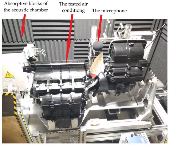
Figure 1.
Testing of the heat, ventilation, and air-conditioning device (HVAC) inside the anechoic chamber, situated in the manufacturing plant of ELCOM, a.s.
The measurement was performed with the use of a Brüel and Kjær Type 4966-H-041 microphone, which is characterised by high measurement accuracy in a wide range of volumes (16.5–134 dB), frequencies (6.3–20,000 Hz) and temperatures (−20–150 °C).
After the measurement, the sound recordings were analysed to depict the pure nature of HVAC sound. The main analysis was undertaken with the use of the discrete Fourier transform:
That converts input signal from time to frequency domain [27]. The length of both sequences is and .
Fourier’s theorem states that any finite sound signal is composed of a set of single-frequency sound waves; namely, the harmonic functions, sine and cosine [28]. The Fourier transform is used to decompose a signal into its individual frequencies, as well as the amplitudes of those frequencies. The result of the Fourier operation is called the spectrum [29]. As can be seen in Figure 2, the achieved results for HVAC show a recorded sample converted to a spectrum.
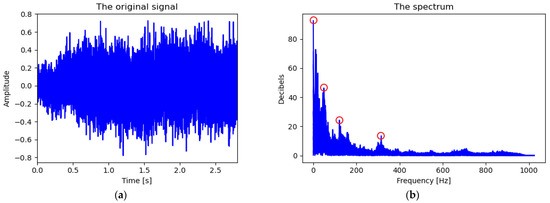
Figure 2.
A sample of recorded HVAC sound (a) and its conversion into spectrum with the help of Fourier transform with pointed peaks (b).
After analysing thousands of available HVAC sound recordings, we can describe the pure nature of HVAC as a composition of elementary harmonic functions. Each of these elementary sine functions is defined as the n-th harmonic function related to frequency of HVAC system’s rotation f and has its origin in a different component or sub-part of the HVAC [30,31]. Figure 2b shows four specific peaks that correspond to four sources of noise. These are the only four sources detected from the results of the thousands of diagnosed sound recordings of the HVAC system: the shaft imbalance of the fan, the unequal electromagnetic field created by each coil of the electric motor, which causes a motor failure, defective bearings, and a defective fan blade. A detailed list of established functions with their presumed sources, that correspond to the described failures with their frequencies, is shown in Table 1. The next step is to compare the amplitudes of peaks with limit values which will show us if it can be qualified as a failure or not.

Table 1.
The list of elementary functions that describe the pure nature of HVAC along with their estimated sources.
These signals make up the base for creating synthetical HVAC sound expressions. For generating such data, we need to define other features of these signals. Since the audibility of these signals is dependent on the factory background noise, we first need to measure the noise inside the chamber, and then set intensities of these signals which are relative to the noise.
2.2. Environmental Noise and Features of the Anechoic Chamber
The sound recording of factory noise that penetrated through walls of the anechoic chamber was recorded inside the chamber. Apart from the exterior noise, other elements of noise, such as influence of flowing blown air, are present during the testing of HVACs. These effects are simulated by mixing pink noise into the recording with the intensity that was observed from real testing. This complete noise is used for generating artificial sounds that simulate testing of the HVACs.
To better illustrate the EN, which is present during in-service testing of HVAC systems, we performed the following experiment, which describes the properties of the acoustic chamber. The measurement was performed inside and outside the acoustic chamber, as shown in Figure 3, at a time when no product was tested, so that we could verify only the properties of the acoustic chamber, respectively the EN, as shown in Figure 4. The damping rate of the chamber depends on the shape and material of its tiling [32,33].
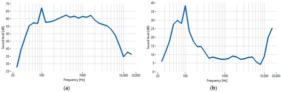
Figure 3.
One-third octave band levels of the sound signal recorded outside (a) and inside (b) the anechoic chamber.
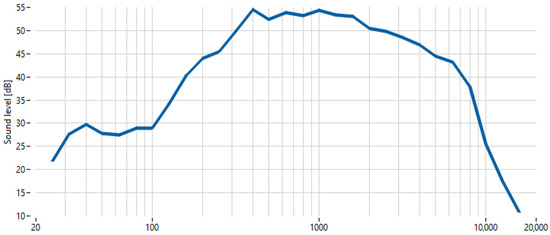
Figure 4.
Absorption level of the anechoic chamber.
Both acquired signals are converted from pressure amplitude to sound pressure level (SPL) on a decibel scale [34], which is usually used in this case, and shown in Figure 3.
The absorption level of anechoic chambers is usually portrayed in a one-third octave band spectrum [35,36]. One-third octave band levels of both signals were calculated for frequencies ranging from 25 Hz to 25 kHz.
The damping level of the anechoic chamber is then calculated as sound level difference between the signal recorded outside and inside of the acoustic chamber according to (2) [37].
As we can see from the Figure 4, the chamber is most effective at damping signals with frequencies ranging from 300 Hz to 2 kHz. The frequencies of EN that are outside of this range strongly influence the effectiveness of the anechoic chamber.
2.3. Elements of Heat, Ventilation, and Air-Conditioning Device (HVAC) Expression
Here, we return to the definition of the elementary expressions of HVACs for generating artificial datasets. It is necessary to determine the amplitude of components and, therefore, the data labeling. With the use of the acquired noise, we can define the amplitude level for all four elementary signals. For each component, we searched the threshold level of amplitude, where the presence of a component is barely recognisable from the noise. These amplitude levels were obtained by an experiment, where we individually merge a component signal of variable amplitude with the noise. Then we listened to the merged signals and tried to recognise the component signal. If the component signal was too strong, we reduced its amplitude. On the other hand, we enhanced the amplitude if we could not recognise the component signal. We did this for all four component signals individually, until we found the thresholds (see signal component nominal amplitude values in Table 2). The listening experiment was performed using a KOSS UR29 headset that provides great volume and is designed to block outside noise. The headset has an impedance of 100 ohms, a sensitivity of 101 dB/mW, and a frequency response range of 18 Hz–20 kHz.
Table 2.
Features of signal components.
By setting the threshold for each possible product defect, we define the point at which the error is subjectively recognisable by a customer. The centre and the duration of the components’ signal were observed from the real measurements of HVACs.
In the real world, some HVAC defects only occur in the narrow range of fan speeds. For quick detection of all defects across the complete working frequency range, the quality control sequence increases the product’s frequency during testing, so it follows the ramp course. The ramp is shown in Figure 5.
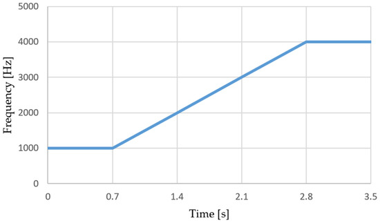
Figure 5.
The ramp course of the testing frequencies during the measuring process.
All components’ parameters have been defined, so we can start to generate the first dataset that will be fed to the neural network. Each sound signal is formed by the noise signal and all four components, where each component feature is randomised by increasing or decreasing its value up to the percentage of the feature’s nominal value. A full list of component features is shown in Table 2.
Before feeding the signals into the network, we need to distinguish sound signals that represent both working and defective HVACs. The purpose of testing HVACs is not to detect a structural flaw, but a defect caused by improper manufacturing. In real testing, an HVAC is categorised as defective if any error appears and can be subjectively noticed by the customer. While the testing completely relies on a customer’s auditory perception, the previous quality control method was based on psychoacoustic tests. Overall, it is not possible to define a dividing parameter based on amplitude or other sound parameters. For this reason, we decided to use CNN algorithms, which do not require any set limits. We will follow this logic and mark each signal as “NOK” if the amplitude of at least one component exceeds its nominal value after randomisation. Otherwise, the signal gets an “OK” tag.
A single dataset consists of 2000 samples evenly distributed across both classes. Each class set is divided into training and testing subsets with a ratio of 5:1. Therefore, each class is represented by 833 training and 167 testing samples.
2.4. Signal Transformation and Datasets Generation
State of the art technology is based on converting an acoustic [38,39] or vibration [40] signal into the spectrogram before feeding it into the neural network. While designing the CNN model for the classification of manufactured products based on their sound expression, various approaches should be considered with some options to begin with. One option is to use a sound recording as a vector input of the neural network.
Since the spectrogram represents the signal in the frequency domain and takes an image format, currently, the best results in the field of the classification of sound recordings are achieved by networks working with input data in the form of images; thus, we decided to try another option to convert a sound recording into an image.
The highest success rate of final classification is usually achieved by transforming the signal into a spectrogram by short-term Fourier transform [41], Mel spectrogram [42] or wavelet spectrogram [43]. Due to the high tack of the HVAC’s quality control process, we used the Gabor transform to make spectrograms [44] as it is considerably faster than the comparable algorithm. The created spectrograms were then scaled according to the Mel scale, which is a scale of pitches that seem to listeners to have equal distance between pitches [45].
Among the transformation parameters, the window length is especially important. With use of this parameter, we can increase the time resolution of the spectrogram while decreasing its frequency resolution, or vice versa. A high value of the window length will highlight long-lasting sound expressions of the original sound signal in a spectrogram, while lower values tend to highlight quick impulses [46]. To avoid omitting any type of sound expression, we will transform the signal into two different spectrograms. Figure 6 shows a spectrogram for the nominal values of EN. The images, which will be processed in the neural network, contain only a spectrogram with no axes. Only two of the four aforementioned HVAC signal components (from Table 2) are barely visible, so we have outlined them using red circles. A complete list of transforming parameters is shown in Table 3.
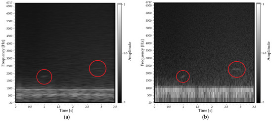
Figure 6.
A sample of sound signal with the nominal level of environmental noise (EN) transformed into spectrogram 1 (a) and spectrogram 2 (b) with pointed HVAC signal components.
Table 3.
Input parameters for creating both spectrogram types by Gabor transform.
All created spectrograms are represented as images with a resolution of 512 × 512 px. While the grey colour map was used for creating the spectrograms, the saved images have only a single channel. Using greyscale images requires only a quarter of memory compared to colour images; thus, further processing is considerably faster [47], which is important for the application. The right choice of using greyscale representation was verified with basic experiments, which showed that the use of colour spectrograms did not result in any increase in classification accuracy, but rather vice versa.
As we mentioned in the introduction, this paper is devoted to finding and describing the influence of EN on the classification accuracy of the decision-making algorithm based on the CNN.
To fulfil the task, we simulated measurements inside superior anechoic chambers that damp more EN. This was done by generating another five datasets. Each dataset simulated a measurement inside an anechoic chamber that could attenuate 2 dB of EN more than the previous one. The best chamber passed −10 dB of EN into the chamber. While the intensity of the generated noise decreased, the sound level of the components’ signal remained constant.
Figure 7 shows the spectrograms of the signal with minimal noise level, which has −10 dB compared to the nominal one. All four signal components of the HVAC are clearly visible in the pictures.
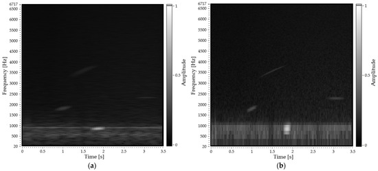
Figure 7.
A sample of spectrogram 1 (a) and spectrogram 2 (b), where intensity of EN is damped to −10 dB from the nominal level.
Similarly, we can simulate measurements inside inferior anechoic chambers that pass more EN to the inside of the chamber. We will also generate five more datasets; however, this time the intensity of EN will increase by 2 dB in every dataset, up to +10 dB in the last one.
As can be seen in Figure 8, the expressions of the HVAC components completely disappeared behind the EN, which was louder by +10 dB compared to the nominal one.
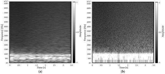
Figure 8.
A sample of spectrogram 1 (a) and spectrogram 2 (b), where intensity of EN is increased to +10 dB from the nominal level.
2.5. Simulations
After defining the format of images that will be entering the neural network, we needed to choose a CNN architecture that will be used in the following simulations. A CNN model usually consists of the following layer types.
The key components of CNN are convolutional layers that perform convolution operations on an input image using a set of kernels [48], where each kernel extracts different regional features from the input images [49]. The output matrices of convolutional layers travel to the pooling layers, which are crucial for the CNN model. This operation not only reduces the dimensions of feature maps, which has a very positive effect on the subsequent computational demands, but also allows the following layers to understand the abstract representation of the image [50]. The dropout layer improves the classification accuracy of the model, by randomly disabling the neurons of all layers during the training phase [51]. Perceptron layers reduce the dimensionality of large feature space [52] into a vector, whose size is equal to the number of available classes.
The training was executed on a single NVIDIA GeForce RTX 2070 graphic card. The card memory was a limiting factor for the size of the CNN architecture used. Initial tests for searching for optimal CNN architecture for our datasets were performed. We found that the best model of a neural network contained four convolution layers interlaced by pooling layers. Then the signal was flattened, and the dropout operation was applied to it. The end of the network consisted of a sequence of three perceptron layers. The complete architecture of the network used, along with a detailed description of the layers’ parameters, is shown in Figure 9.
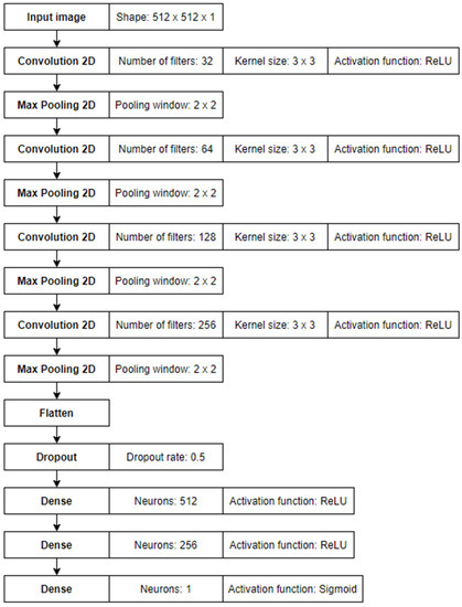
Figure 9.
Neural network architecture.
While searching for optimal CNN architecture, we selected the standard VGG16 [53], which we modified for our dataset. Similar modifications of this neural network type were described in [54,55]. This neural network type illustrates a growing trend in a number of kernels in convolution layers, and conversely a decreasing trend in a number of the perceptron layers of neutrons with the increasing depth of the network. We tested the specific structure optimisation by reducing the number of included layers as well as the size of these layers. However, no simpler architecture achieved at least the same quality as our selected model.
In future work, we will optimise the CNN model, for example by a genetic algorithm [56,57], to reduce its size and processing time, while maintaining great accuracy rates that are obtained by the currently proposed model. This optimisation is beyond the scope of this contribution.
During the training of the network, the global minimum of the loss function is searched by the RMSprop [58] optimisation algorithm with a learning rate of . We experimented with other combinations of the optimisation algorithms, such as Adam [59], AdaGrad [60], Adadelta [61] and AdaMax [59], with various values of learning rate , but none of these combinations proved to be better than the aforementioned one. The input images enter the network in batches of eight images, which is a maximally permissible value for our architecture and available GPU, since we need to avoid an out-of-memory error. The training phase consists of 50 epochs, but the results present the highest classification accuracy achieved across those epochs. A test dataset was used for verification.
The last layer of the used CNN model contains a single neuron that relies on a Sigmoid activation function [62], thus neuron value varies from 0 to 1. The sample is classified as class according to (3).
The classification accuracy of the model on whole dataset is evaluated by (4)
where is the number of correctly classified samples from the dataset and is the total amount of dataset samples. A sample is correctly classified if its predicted class is equal to the ground truth class, that was assigned to the sample during the generation.
3. Results and Discussion
The total number of generated datasets was 22 per spectrogram type, where the intensity of noise gradually grew from −10 dB to +10 dB with steps of 2 dB. To eliminate any statistical errors from the classification accuracy of a trained neural network, the training was performed multiple times for all datasets. The first experiments were done on datasets with images of spectrogram 1.
Table 4 shows a list of classification accuracies, in percentages, that the CNN could reach from training on a particular dataset with data in the form of spectrogram 1. Graphical representation of the classification accuracy trend is detailed in Figure 10, which helps us to obtain a better image of the relationship between environmental noise and classification accuracy.
Table 4.
Obtained classification accuracies [%] for datasets of spectrogram 1.
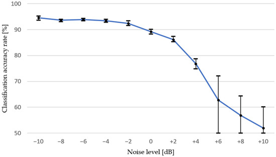
Figure 10.
Trend of classification accuracy across all tested intensities of EN for data represented by spectrogram 1.
The same experiment was done on datasets with data in the form of spectrogram 2. Numerical value accuracy rates are presented in Table 5 and the graphical trend is shown in Figure 11.
Table 5.
Obtained classification accuracies [%] for datasets of spectrogram 2.
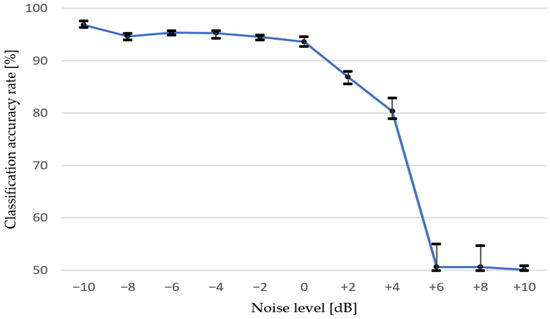
Figure 11.
Trend of classification accuracy across all tested intensities of EN for data represented by spectrogram 2.
The results describe the influence of environmental noise on the assembly line to the classification accuracy of a quality control algorithm based on a convolutional neural network. Both graphs show that decreasing the intensity of environmental noise from the nominal value leads to slight improvements of classification accuracy, and these results are very stable across multiple runs. On the other hand, increasing the same amount of the noise level has a greater impact on reducing accuracy rates.
Sound recordings transformed to spectrograms 1, which have greater window length, tend to decrease the accuracy rate with noise increasing more or less linearly. On the contrary, a neural network trained on data transformed by spectrograms 2 could process slightly noisy records, but from +6 dB of nominal noise level, it could not learn any credible decision-making criterion, thus confirming the classical analytical method results. Simply put, the noise on this kind of spectrogram tends to overdraw the signal components’ expressions more aggressively. For a direct comparison of both spectrogram types, see Figure 12.
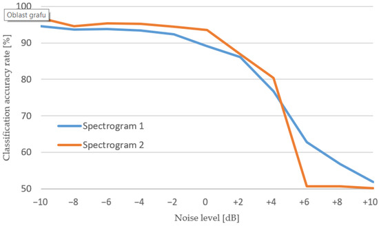
Figure 12.
Comparison of both spectrogram types with regard to classification accuracy.
Overall, the greater the noise level, the less stable the results of classification were across multiple runs. Both spectrogram types sometimes failed to learn anything from the data and returned just 50% classification accuracy in very noisy datasets. This happened quite often to data from spectrogram 2. On the other hand, with the use of this type of spectrogram, the network reached its highest accuracy rates on less noisy data by approximately 2%, compared to data transformed by spectrogram 1.
4. Conclusions
We have diagnosed thousands of HVAC system samples and have found out unique sources of failures. Thanks to this we have been able to create synthetic recordings of specific failure sources which correspond to the measured harmonic frequencies. Here, we have converted the sound recordings into images using spectrograms, which are more suitable for diagnostics using neural networks. We have generated a total of 11 datasets, where each of them simulates a measurement in an anechoic chamber with various levels of EN damping.
From these findings, we can deduce a logical conclusion, that using a CNN architecture that can input multiple spectrograms of the same sound recording at the same time, which complement each other, should lead to an increased classification accuracy rate. Another improvement can be made by finding the ideal combination of spectrogram parameters and architecture of neural networks. This complex problem is far beyond the scope of this article. It will, however, be addressed in the forthcoming research.
The next area of further research is searching for a smaller and thus faster CNN model, that will be ideally suited for our task. The optimal architecture will be searched mainly by a genetic algorithm.
This contribution should be useful for companies that focus on production and testing of rotary devices directly at the production line and want to upgrade their anechoic chamber to improve the current quality control process. Considering the life cycle of the anechoic chambers installed directly in production lines could be up to six years, future research gives us a large amount of data for concluding the findings and future improvements. It will also help the manufacturers to make a decision about purchasing a better anechoic chamber—which would filter more EN—by having an estimate on the improvement level of the accuracy rate that can be gained by the upgrade every time a new production line is planned for a new model of HVAC device production.
The currently used qualification algorithm can distinguish faulty devices, and future work will show us also the cause of the failure, pointing out the source of the noise. Further research will focus on extending the use of the described methodology to different types of device using rotary mechanisms, either HVAC used outside the automotive industry, for example marine and aircraft technology, or general devices used for home appliances.
Author Contributions
Conceptualization, J.S.; methodology, J.S. and J.Š.; software, J.S. and J.Š.; validation, J.S., L.L. and J.Š.; formal analysis, J.S., R.W. and L.L.; investigation, J.S., L.L.; resources, J.S. and R.W.; data curation, J.S.; writing—original draft preparation, J.S., L.L. and R.W.; writing—review and editing, J.S., R.W. and L.L.; visualization, J.S.; supervision, J.Š., R.W. and S.W.; project administration, R.W., L.L.; funding acquisition, R.W. All authors have read and agreed to the published version of the manuscript.
Funding
This work was supported by the European Regional Development Fund in the Research Centre of Advanced Mechatronic Systems project, CZ.02.1.01/0.0/0.0/16_019/0000867 within the Operational Programme Research, Development and Education and the project SP2021/27 Advanced methods and technologies in the field of machine and process control supported by the Ministry of Education, Youth and Sports, Czech Republic.
Institutional Review Board Statement
Not applicable.
Informed Consent Statement
Not applicable.
Data Availability Statement
Contact correspondence author.
Conflicts of Interest
The authors declare no conflict of interest. The funders had no role in the design of the study; in the collection, analyses, or interpretation of data; in the writing of the manuscript, or in the decision to publish the results.
References
- Dalenogare, L.S.; Benitez, G.B.; Ayala, N.F.; Frank, A.G. The expected contribution of Industry 4.0 technologies for industrial performance. Int. J. Prod. Econ. 2018, 204, 383–394. [Google Scholar] [CrossRef]
- Grollmisch, S.; Abeßer, J.; Liebetrau, J.; Lukashevich, H. Sounding Industry: Challenges and Datasets for Industrial Sound Analysis. In Proceedings of the 2019 27th European Signal Processing Conference (EUSIPCO), A Coruna, Spain, 2–6 September 2019; pp. 1–5. [Google Scholar] [CrossRef]
- Hosseini, S.M.; Ataei, M.; Khalokakaei, R.; Mikaeil, R.; Haghshenas, S.S. Study of the effect of the cooling and lubricant fluid on the cutting performance of dimension stone through artificial intelligence models. Eng. Sci. Technol. Int. J. 2020, 23, 71–81. [Google Scholar] [CrossRef]
- Xu, F.; Uszkoreit, H.; Du, Y.; Fan, W.; Zhao, D.; Zhu, J. Explainable AI: A Brief Survey on History, Research Areas, Approaches and Challenges. In Natural Language Processing and Chinese Computing; Spinger: Cham, Switzerland, 2019; pp. 563–574. [Google Scholar] [CrossRef]
- Ciaburro, G. Sound Event Detection in Underground Parking Garage Using Convolutional Neural Network. Big Data Cogn. Comput. 2020, 4, 20. [Google Scholar] [CrossRef]
- Ciaburro, G.; Iannace, G. Improving Smart Cities Safety Using Sound Events Detection Based on Deep Neural Network Algorithms. Informatics 2020, 7, 23. [Google Scholar] [CrossRef]
- Shi, B.; Sun, M.; Kao, C.-C.; Rozgic, V.; Matsoukas, S.; Wang, C. Compression of Acoustic Event Detection Models with Low-rank Matrix Factorization and Quantization Training. arXiv 2019, arXiv:1905.00855. Available online: http://arxiv.org/abs/1905.00855 (accessed on 27 March 2021).
- Kao, C.-C.; Wang, W.; Sun, M.; Wang, C. R-CRNN: Region-based Convolutional Recurrent Neural Network for Audio Event Detection. arXiv 2018, arXiv:1808.06627. Available online: http://arxiv.org/abs/1808.06627 (accessed on 27 March 2021).
- Johnson, D.S.; Grollmisch, S. Techniques Improving the Robustness of Deep Learning Models for Industrial Sound Analysis. In Proceedings of the 2020 28th European Signal Processing Conference (EUSIPCO), Amsterdam, The Netherlands, 18–21 January 2021; pp. 81–85. [Google Scholar] [CrossRef]
- Tan, A.; Salim, N.; Hidayah, N.; Azhan, S.; Ismail, M. ANGKASA Reverberation Acoustic Chamber Characterization. WSEAS Trans. Signal Process. 2017, 13, 275–280. [Google Scholar]
- Huang, H.B.; Wu, J.H.; Huang, X.R.; Yang, M.L.; Ding, W.P. The development of a deep neural network and its application to evaluating the interior sound quality of pure electric vehicles. Mech. Syst. Signal Process. 2019, 120, 98–116. [Google Scholar] [CrossRef]
- Swart, D.J.; Bekker, A.; Bienert, J. The subjective dimensions of sound quality of standard production electric vehicles. Appl. Acoust. 2018, 129, 354–364. [Google Scholar] [CrossRef]
- Huang, H.B.; Wu, J.H.; Huang, X.R.; Ding, W.P.; Yang, M.L. A novel interval analysis method to identify and reduce pure electric vehicle structure-borne noise. J. Sound Vib. 2020, 475, 115258. [Google Scholar] [CrossRef]
- Flor, D.; Pena, D.; Pena, L.; de Sousa, V.A.; Martins, A. Characterization of Noise Level Inside a Vehicle under Different Conditions. Sensors 2020, 20, 2471. [Google Scholar] [CrossRef]
- Qian, K.; Hou, Z.; Liang, J.; Liu, R.; Sun, D. Interior Sound Quality Prediction of Pure Electric Vehicles Based on Transfer Path Synthesis. Appl. Sci. 2021, 11, 4385. [Google Scholar] [CrossRef]
- Ma, C.; Chen, C.; Liu, Q.; Gao, H.; Li, Q.; Gao, H.; Shen, Y. Sound Quality Evaluation of the Interior Noise of Pure Electric Vehicle Based on Neural Network Model. IEEE Trans. Ind. Electron. 2017, 64, 9442–9450. [Google Scholar] [CrossRef]
- Oliinyk, B.; Oleksiuk, V. Automation in software testing, can we automate anything we want? 2019, 2546, 224–234. Available online: http://dspace.tnpu.edu.ua/handle/123456789/16779 (accessed on 8 July 2021).
- Reis, D.; Vanzo, F.; Reis, J.; Duarte, M. Discriminant Analysis and Optimization Applied to Vibration Signals for the Quality Control of Rotary Compressors in the Production Line. Arch. Acoust. 2019, 44, 79–81. [Google Scholar] [CrossRef]
- Han, S.; Choi, H.-J.; Choi, S.-K.; Oh, J.-S. Fault Diagnosis of Planetary Gear Carrier Packs: A Class Imbalance and Multiclass Classification Problem. Int. J. Precis. Eng. Manuf. 2019, 20, 167–179. [Google Scholar] [CrossRef]
- Albawi, S.; Mohammed, T.A.; Al-Zawi, S. Understanding of a convolutional neural network. In Proceedings of the 2017 International Conference on Engineering and Technology (ICET), Antalya, Turkey, 21–23 August 2017; pp. 1–6. [Google Scholar] [CrossRef]
- Copiaco, A.; Ritz, C.; Abdulaziz, N.; Fasciani, S. A Study of Features and Deep Neural Network Architectures and Hyper-Parameters for Domestic Audio Classification. Appl. Sci. 2021, 11, 4880. [Google Scholar] [CrossRef]
- Khumaidi, A.; Yuniarno, E.M.; Purnomo, M.H. Welding defect classification based on convolution neural network (CNN) and Gaussian kernel. In Proceedings of the 2017 International Seminar on Intelligent Technology and Its Applications (ISITIA), Surabaya, Indonesia, 28–29 August 2017; pp. 261–265. [Google Scholar] [CrossRef]
- Zhiqiang, W.; Jun, L. A review of object detection based on convolutional neural network. In Proceedings of the 2017 36th Chinese Control Conference (CCC), Dalian, China, 26–28 July 2017; pp. 11104–11109. [Google Scholar] [CrossRef]
- Park, S.; Jeong, Y.; Kim, H.S. Multiresolution CNN for reverberant speech recognition. In Proceedings of the 2017 20th Conference of the Oriental Chapter of the International Coordinating Committee on Speech Databases and Speech I/O Systems and Assessment (O-COCOSDA), Seoul, Korea, 1–3 November 2017; pp. 1–4. [Google Scholar] [CrossRef]
- Kwon, G.; Jo, H.; Kang, Y.J. Model of psychoacoustic sportiness for vehicle interior sound: Excluding loudness. Appl. Acoust. 2018, 136, 16–25. [Google Scholar] [CrossRef]
- Technology Solutions Provider. Intelligence Inside. ELCOM. Available online: https://www.elcom.cz/ (accessed on 7 July 2021).
- Cochran, W.T.; Cooley, J.W.; Favin, D.L.; Helms, H.D.; Kaenel, R.A.; Lang, W.W.; Maling, G.C.; Nelson, D.E.; Rader, C.M.; Welch, P.D. What is the fast Fourier transform? Proc. IEEE 1967, 55, 1664–1674. [Google Scholar] [CrossRef]
- Domínguez, A. Highlights in the History of the Fourier Transform [Retrospectroscope]. IEEE Pulse 2016, 7, 53–61. [Google Scholar] [CrossRef]
- Kay, S.M.; Marple, S.L. Spectrum analysis—A modern perspective. Proc. IEEE 1981, 69, 1380–1419. [Google Scholar] [CrossRef]
- Hundy, G.F.; Trott, A.R.; Welch, T.C. Chapter 24—Air Conditioning Methods and Applications. In Refrigeration, Air Conditioning and Heat Pumps, 5th ed.; Hundy, G.F., Trott, A.R., Welch, T.C., Eds.; Butterworth-Heinemann: Oxford, UK, 2016; pp. 375–392. [Google Scholar] [CrossRef]
- Alipouri, Y.; Zhong, L. Multi-Model Identification of HVAC System. Appl. Sci. 2012, 11, 668. [Google Scholar] [CrossRef]
- Nejad, M.E.T.; Loghmani, A.; Ziaei-Rad, S. The effects of wedge geometrical parameters and arrangement on the sound absorption coefficient—A numerical and experimental study. Appl. Acoust. 2020, 169, 107458. [Google Scholar] [CrossRef]
- Pawlenka, M.; Mahdal, M.; Tuma, J.; Burecek, A. Application of a Bandpass Filter for the Active Vibration Control of High-Speed Rotors. Int. J. Acoust. Vib. 2019, 24, 608–615. [Google Scholar] [CrossRef]
- Hughes, L.F. The Fundamentals of Sound and its Measurement. J. Am. Assoc. Lab. Anim. Sci. 2007, 46, 14–19. [Google Scholar] [PubMed]
- Ghanavi, R.; Cabrera, D. A broadband point source loudspeaker design and its application to anechoic chamber qualification. Appl. Acoust. 2021, 178, 107994. [Google Scholar] [CrossRef]
- Wijnant, Y.H.; Kuipers, E.R.; de Boer, A. Development and Application of a New Method for the Insitu Measurement of Sound Absorption; Katholieke Universiteit Leuven: Leuven, Belgium, 2010; Volume 31, pp. 109–122. [Google Scholar]
- Pindoriya, R.M.; Rajpurohit, B.S.; Kumar, R. Design and Performance Analysis of Low Cost Acoustic Chamber for Electric Machines. In Proceedings of the 2018 IEEE 8th Power India International Conference (PIICON), Kurukshetra, India, 10–12 December 2018; pp. 1–5. [Google Scholar] [CrossRef]
- Jaiswal, K.; Patel, D.K. Sound Classification Using Convolutional Neural Networks. In Proceedings of the 2018 IEEE International Conference on Cloud Computing in Emerging Markets (CCEM), Bangalore, India, 23–24 November 2018; pp. 81–84. [Google Scholar] [CrossRef]
- Khamparia, A.; Gupta, D.; Nguyen, N.G.; Khanna, A.; Pandey, B.; Tiwari, P. Sound Classification Using Convolutional Neural Network and Tensor Deep Stacking Network. IEEE Access 2019, 7, 7717–7727. [Google Scholar] [CrossRef]
- Pham, M.T.; Kim, J.-M.; Kim, C.H. Accurate Bearing Fault Diagnosis under Variable Shaft Speed using Convolutional Neural Networks and Vibration Spectrogram. Appl. Sci. 2020, 10, 6385. [Google Scholar] [CrossRef]
- Durak, L.; Arikan, O. Short-time Fourier transform: Two fundamental properties and an optimal implementation. IEEE Trans. Signal Process. 2003, 51, 1231–1242. [Google Scholar] [CrossRef]
- Zhang, J.; Ling, Z.; Liu, L.; Jiang, Y.; Dai, L. Sequence-to-Sequence Acoustic Modeling for Voice Conversion. IEEE/ACM Trans. Audio Speech Lang. Process. 2019, 27, 631–644. [Google Scholar] [CrossRef] [Green Version]
- Selesnick, I.W.; Baraniuk, R.G.; Kingsbury, N.C. The dual-tree complex wavelet transform. IEEE Signal Process. Mag. 2005, 22, 123–151. [Google Scholar] [CrossRef] [Green Version]
- Qian, S.; Chen, D. Discrete Gabor transform. IEEE Trans. Signal Process. 1993, 41, 2429–2438. [Google Scholar] [CrossRef] [Green Version]
- Stevens, S.S.; Volkmann, J. The Relation of Pitch to Frequency: A Revised Scale on JSTOR. Available online: https://www.jstor.org/stable/1417526?seq=1 (accessed on 28 October 2020).
- Zhang, X.; Chen, A.; Zhou, G.; Zhang, Z.; Huang, X.; Qiang, X. Spectrogram-frame linear network and continuous frame sequence for bird sound classification. Ecol. Inform. 2019, 54, 101009. [Google Scholar] [CrossRef]
- Bradski, G.; Kaehler, A. Learning OpenCV: Computer Vision in C++ with the OpenCV Library, 2nd ed.; O’Reilly Media, Inc.: Sebastopol, CA, USA, 2013. [Google Scholar]
- Kuo, C.-C.J. Understanding convolutional neural networks with a mathematical model. J. Vis. Commun. Image Represent. 2016, 41, 406–413. [Google Scholar] [CrossRef] [Green Version]
- Li, Q.; Cai, W.; Wang, X.; Zhou, Y.; Feng, D.D.; Chen, M. Medical image classification with convolutional neural network. In Proceedings of the 2014 13th International Conference on Control Automation Robotics Vision (ICARCV), Singapore, 10–12 December 2014; pp. 844–848. [Google Scholar] [CrossRef]
- Zhai, S.; Wu, H.; Kumar, A.; Cheng, Y.; Lu, Y.; Zhang, Z.; Feris, R. S3Pool: Pooling with Stochastic Spatial Sampling. In Proceedings of the 2017 IEEE Conference on Computer Vision and Pattern Recognition (CVPR), Honolulu, Hawaii, 21–26 July 2017; pp. 4003–4011. [Google Scholar] [CrossRef] [Green Version]
- Dahl, G.E.; Sainath, T.N.; Hinton, G.E. Improving deep neural networks for LVCSR using rectified linear units and dropout. In Proceedings of the 2013 IEEE International Conference on Acoustics, Speech and Signal. Processing, Vancouver, BC, Canada, 26–31 May 2013; pp. 8609–8613. [Google Scholar] [CrossRef] [Green Version]
- Zhang, Z.; Lyons, M.; Schuster, M.; Akamatsu, S. Comparison between geometry-based and Gabor-wavelets-based facial expression recognition using multi-layer perceptron. In Proceedings of the Third IEEE International Conference on Automatic Face and Gesture Recognition, Nara, Japan, 11–16 April 1998; pp. 454–459. [Google Scholar] [CrossRef]
- Simonyan, K.; Zisserma, A.N. Very Deep Convolutional Networks for Large-Scale Image Recognition. arXiv 2014, arXiv:1409.1556. Available online: http://arxiv.org/abs/1409.1556 (accessed on 23 July 2021).
- Cao, X.; Togneri, R.; Zhang, X.; Yu, Y. Convolutional Neural Network with Second-Order Pooling for Underwater Target Classification. IEEE Sens. J. 2018, 19, 3058–3066. Available online: https://ieeexplore.ieee.org/abstract/document/8573835 (accessed on 23 July 2021). [CrossRef]
- Wattanavichean, N.; Boonchai, J.; Yodthong, S.; Preuksakarn, C.; Huang, C.-H.; Surasak, T. GFP Pattern Recognition in Raman Spectra by Modified VGG Networks for Localisation Tracking in Living Cells. Eng. J. 2021, 25, 151–160. [Google Scholar] [CrossRef]
- Bouktif, S.; Fiaz, A.; Ouni, A.; Serhani, M.A. Optimal Deep Learning LSTM Model for Electric Load Forecasting using Feature Selection and Genetic Algorithm: Comparison with Machine Learning Approaches. Energies 2008, 11, 1636. [Google Scholar] [CrossRef] [Green Version]
- Supraja, P.; Gayathri, V.M.; Pitchai, R. Optimized neural network for spectrum prediction using genetic algorithm in cognitive radio networks. Cluster Comput. 2019, 22, 157–163. [Google Scholar] [CrossRef]
- Lecture 6.5-rmsprop: Divide the Gradient by a Running Average of Its Recent Magnitude—AMiner. Available online: https://www.aminer.org/pub/5b076eb4da5629516ce741dc/lecture-rmsprop-divide-the-gradient-by-a-running-average-of-its-recent (accessed on 7 October 2020).
- Kingma, D.; Ba, J. Adam: A Method for Stochastic Optimization. arXiv 2014, arXiv:1412.6980. [Google Scholar]
- Duchi, J.; Hazan, E.; Singer, Y. Adaptive Subgradient Methods for Online Learning and Stochastic Optimization. J. Mach. Learn. Res. 2011, 12, 2121–2159. [Google Scholar]
- Zeiler, M.D. ADADELTA: An Adaptive Learning Rate Method. arXiv 2012, arXiv:1212.5701. Available online: http://arxiv.org/abs/1212.5701 (accessed on 7 October 2020).
- Narayan, S. The generalized sigmoid activation function: Competitive supervised learning. Inf. Sci. 1997, 99, 69–82. [Google Scholar] [CrossRef]
Publisher’s Note: MDPI stays neutral with regard to jurisdictional claims in published maps and institutional affiliations. |
© 2021 by the authors. Licensee MDPI, Basel, Switzerland. This article is an open access article distributed under the terms and conditions of the Creative Commons Attribution (CC BY) license (https://creativecommons.org/licenses/by/4.0/).