
Optimised Extraction of Archaeological Features from Full 3-D GPR Data

 , ,
, , 
Abstract
:1. Introduction
- (1)
- Achieve optimized information that is directly useful for archaeologists for planning excavation, often in areas where irregular and already excavated areas are present.
- (2)
- Image complex structures in which many superimposed and irregular structures are present.
- (3)
- Obtain full georeferenced results that are easy to understand and manage even by end-users and those who are not trained in geophysics.
- (4)
- Validate geophysical results with excavations and evaluate the intrinsic resolution limits of GPR by comparing its results with excavations.
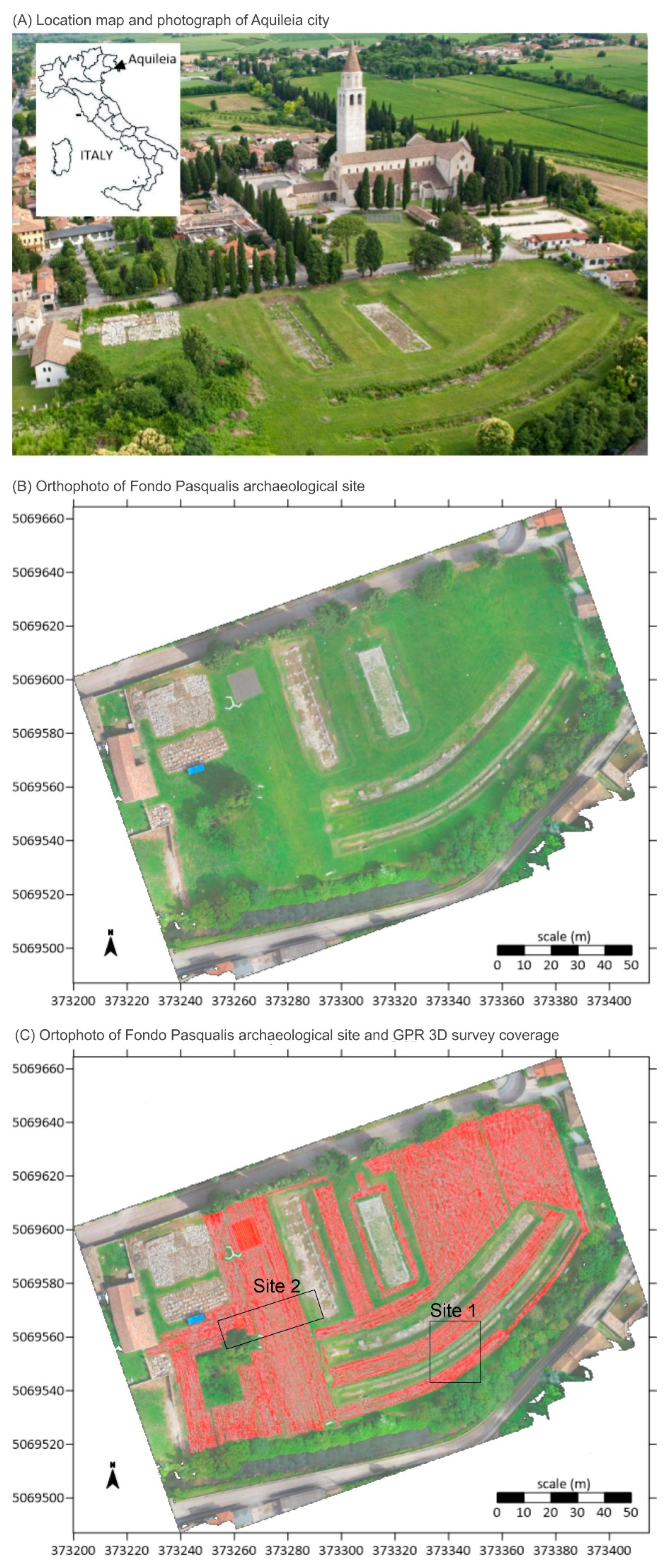
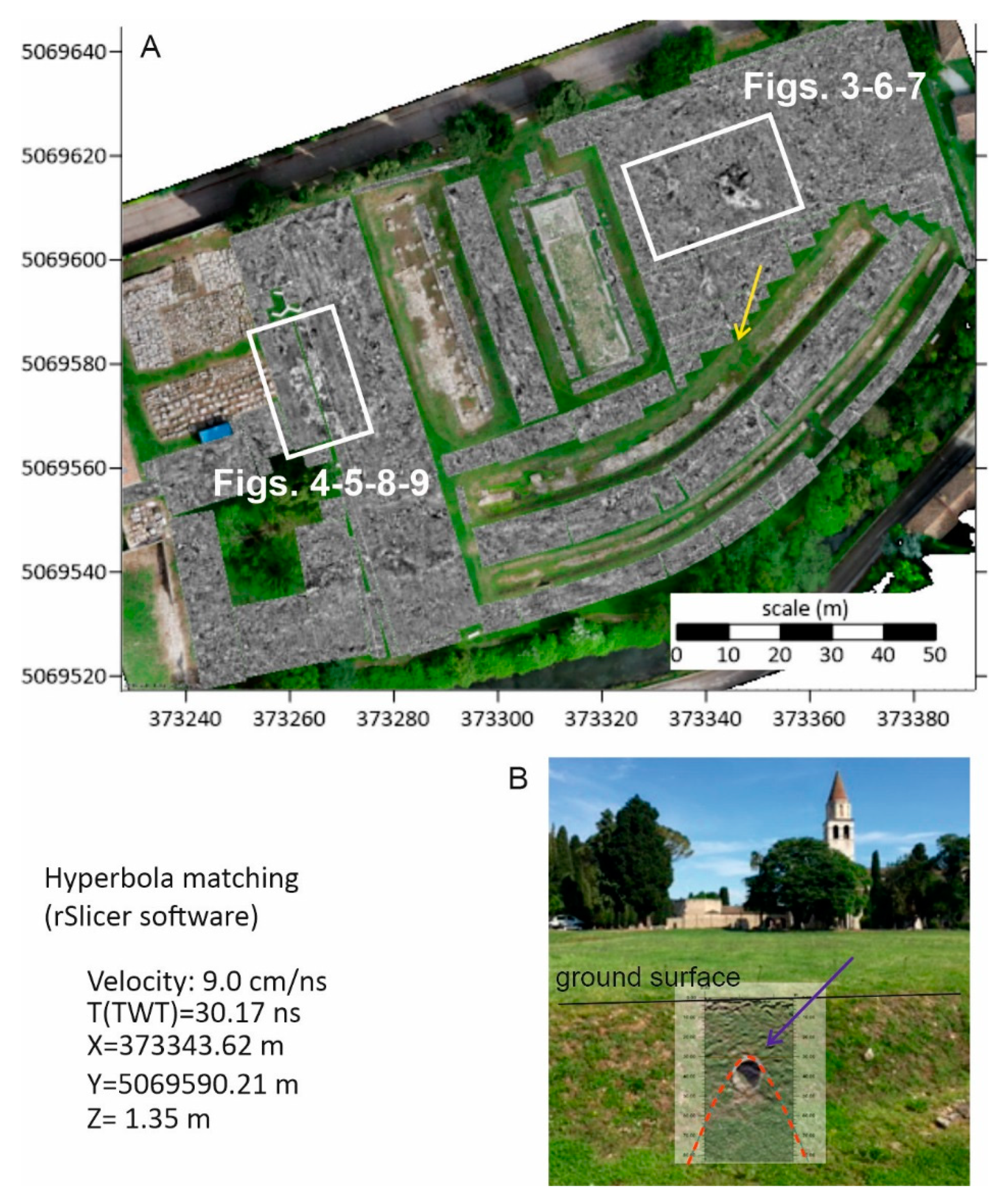
2. Test Site
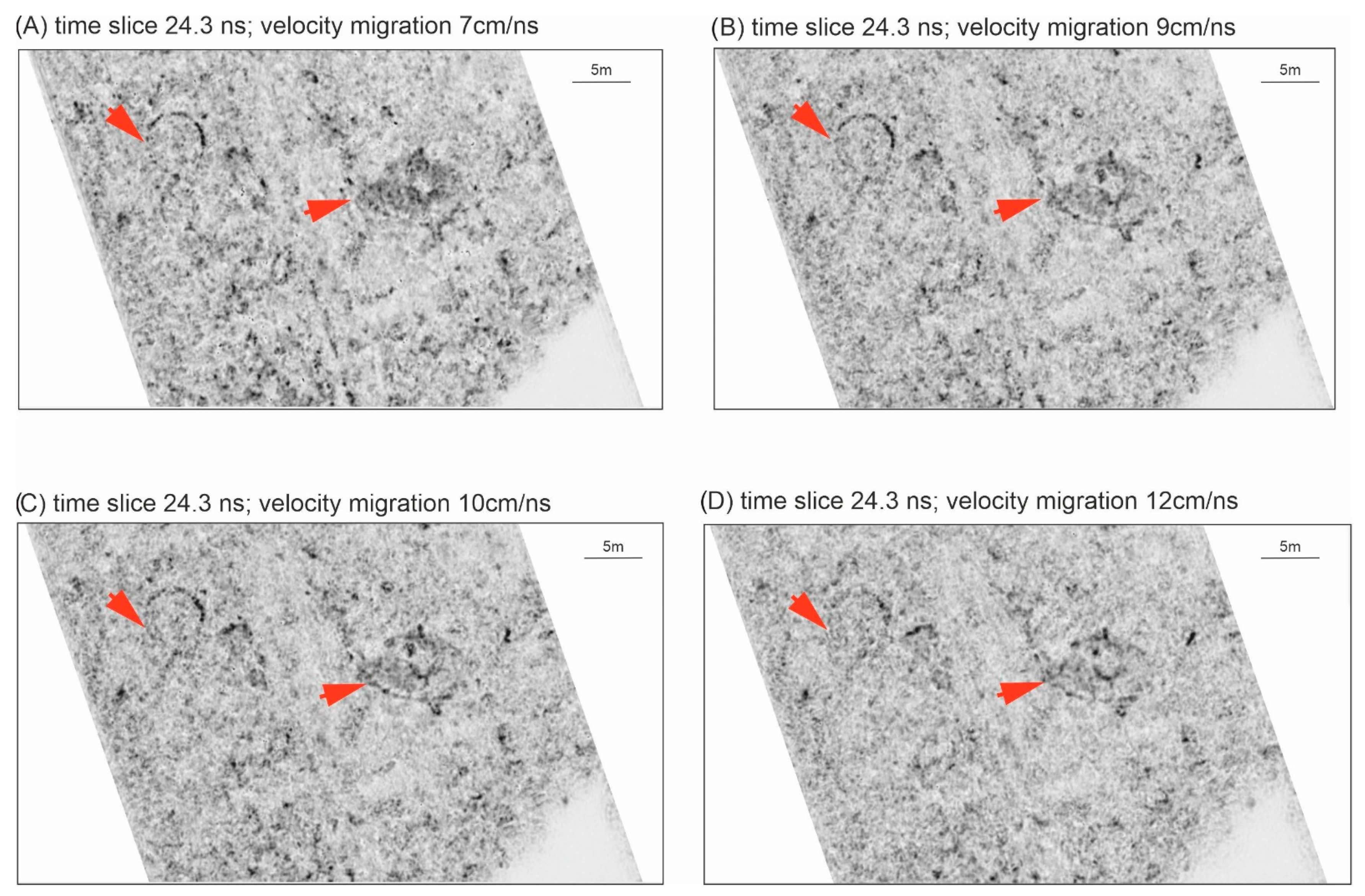
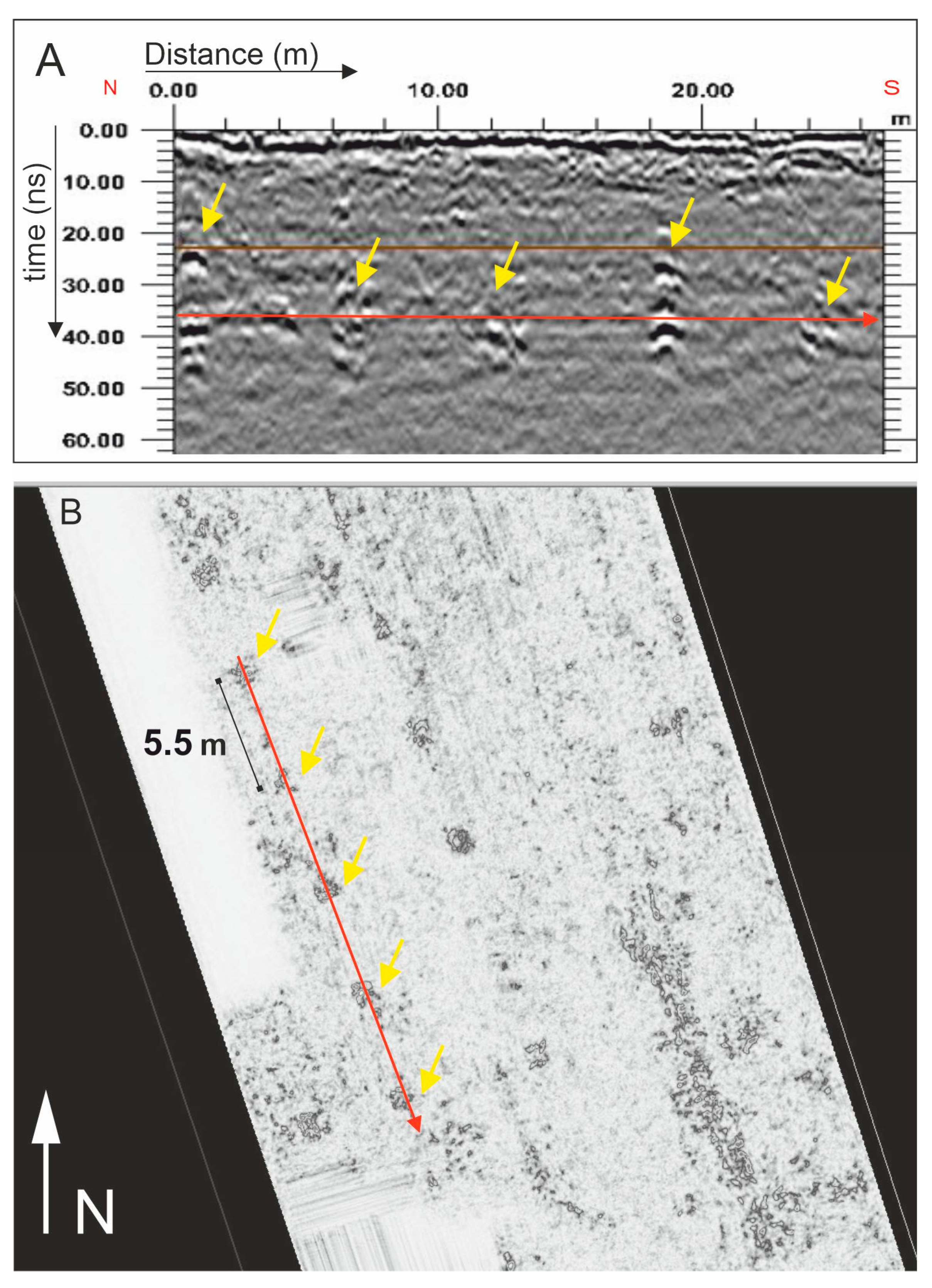
3. Methods
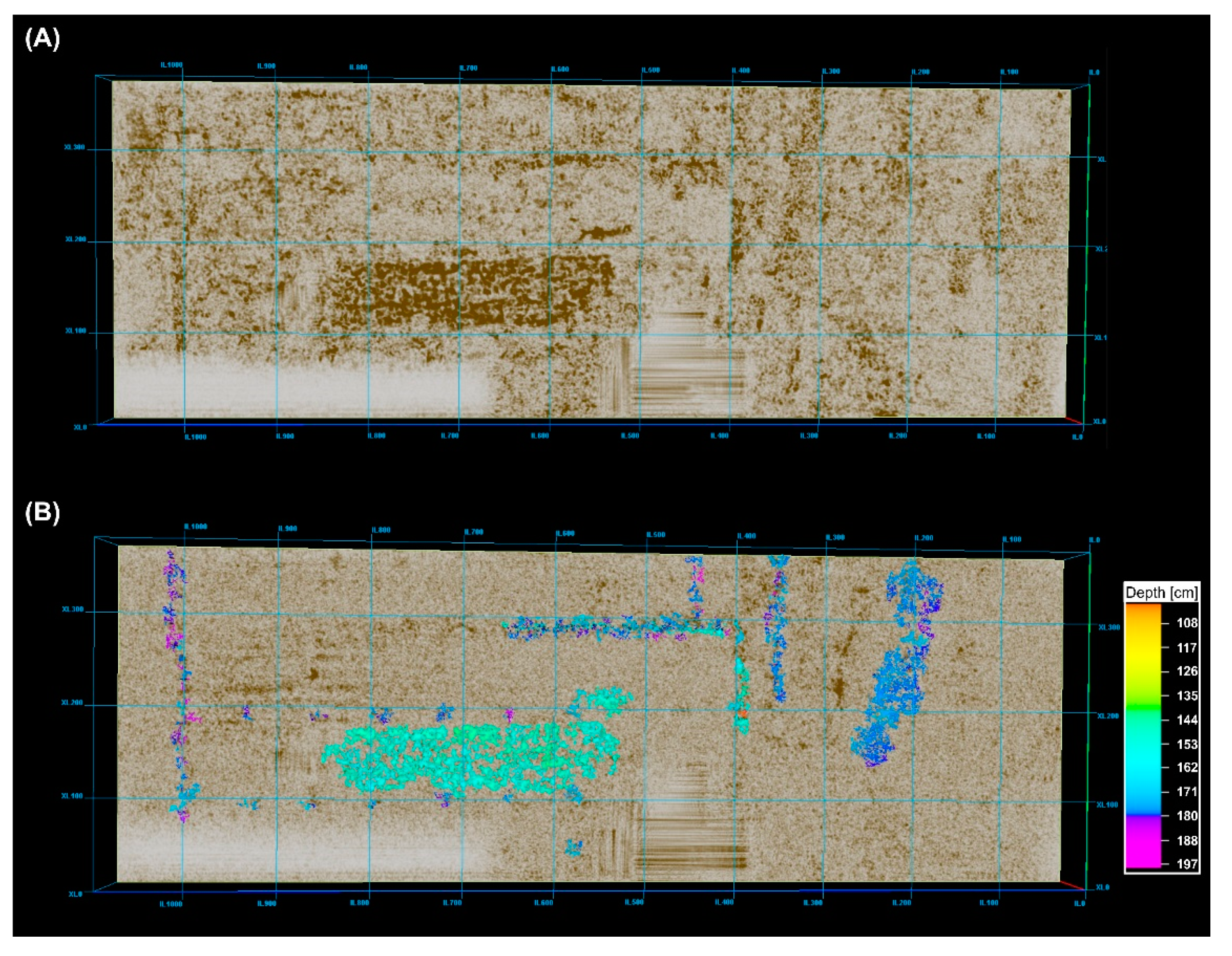
4. Results
5. Discussion
6. Conclusions
- -
- Storage of all the data in the same digital suite;
- -
- Integrated analyses and correlation of events with the results coming from the new excavated areas.
Author Contributions
Funding
Institutional Review Board Statement
Informed Consent Statement
Data Availability Statement
Acknowledgments
Conflicts of Interest
References
- Conyers, L.B. Ground-Penetrating Radar for Geoarchaeology; Wiley: Hoboken, NJ, USA, 2016. [Google Scholar] [CrossRef]
- Jol, H.M. Ground Penetrating Radar: Theory and Applications; Elsevier Science Ltd.: Amsterdam, The Netherlands, 2009; 524p. [Google Scholar]
- Schmidt, A. Earth Resistance for Archaeologists, (Vol. 3 of Geophysical Methods for Archaeology); Rowman & Littlefield: New York, NY, USA, 2013; 195p, ISBN 0759112045. [Google Scholar]
- Aspinall, A.; Gaffney, C.; Schmidt, A. (Eds.) Magnetometry for Archaeologists; Altamira Press: New York, NY, USA, 2008; 208p, ISBN 0-7591-1106-5. [Google Scholar]
- Nardi, I.; Lucchi, E.; de Rubeis, T.; Ambrosini, D. Quantification of heat energy losses through the building envelope: A state-of-the-art analysis with critical and comprehensive review on infrared thermography. Build. Environ. 2018, 146, 190–205. [Google Scholar] [CrossRef] [Green Version]
- Kalayci, T.; Lasaponara, R.; Wainwright, J.; Masini, N. Multispectral Contrast of Archaeological Features: A Quantitative Evaluation. Remote Sens. 2019, 11, 913. [Google Scholar] [CrossRef] [Green Version]
- Conyers, L.B. Ground-penetrating Radar for Archaeological Mapping. In Remote Sensing in Archaeology; Wiseman, J., El-Baz, F., Eds.; Interdisciplinary Contributions To Archaeology; Springer: New York, NY, USA, 2006. [Google Scholar] [CrossRef]
- Zhao, W.; Tian, G.; Wang, B.; Forte, E.; Pipan, M.; Lin, J.; Shi, Z.; Li, X. 2D and 3D imaging of a buried prehistoric canoe using GPR attributes: A case study. Near Surf. Geophys. 2013, 11, 457–464. [Google Scholar] [CrossRef]
- Ortega-Ramírez, J.; Bano, M.; Alvarado, L.V.; Martínez, D.M.; Rivero-Chong, R.; MotoliníaTemol, C. High-resolution 3-D GPR applied in the diagnostic of the detachment and cracks in pre-Hispanic mural paintings at “Templo Rojo”, Cacaxtla, Tlaxcala, Mexico. J. Cult. Herit. 2021, 50, 61–72. [Google Scholar] [CrossRef]
- Annan, A. Applications of ground penetrating radar in archaeological and forensic contexts. First Break. 2004, 22, 9. [Google Scholar] [CrossRef]
- Goodman, D.; Nishimura, Y.; Rogers, J.D. GPR time-slices in archaeological prospection. Archaeol. Prospect. 1995, 2, 85–89. [Google Scholar]
- Leckebusch, J. Ground-penetrating radar: A modern three-dimensional prospection method. Archaeol. Prospect. 2003, 10, 213–240. [Google Scholar] [CrossRef]
- Grasmueck, M.; Weger, R.; Horstmeyer, H. How dense is dense enough for a real 3D GPR survey? In Proceedings of the 2003 SEG Annual Meeting, Dallas, TX, USA, 26–31 October 2003. [Google Scholar]
- Grasmueck, M.; Weger, R.; Horstmeyer, H. 2004, Full-resolution 3D GPR imaging for geoscience and archeology. In Proceedings of the Tenth International Conference on Grounds Penetrating Radar, GPR 2004, Delft, The Netherlands, 21–24 June 2004; pp. 329–332. [Google Scholar]
- Grasmueck, M.; Weger, R.; Horstmeyer, H. Full-resolution 3D GPR imaging. Geophysics 2005, 70, K12–K19. [Google Scholar] [CrossRef]
- Neubauer, W.; Eder-Hinterleitner, A.; Seren, S.; Melichar, P. Georadar in the Roman civil town Carnuntum, Austria: An approach for archaeological interpretation of GPR data. Archaeol. Prospect. 2002, 9, 135–156. [Google Scholar] [CrossRef]
- Booth, A.D.; Linford, N.T.; Clark, R.A.; Murray, T. Three-dimensional, multi-offset GPR imaging of archaeological targets. Archaeol. Prospect. 2008, 15, 1–20. [Google Scholar] [CrossRef]
- Zhao, W.; Forte, E.; Pipan, M.; Tian, G. Ground Penetrating Radar (GPR) attribute analysis for archaeological prospection. J. Appl. Geophys. 2013, 97, 107–117. [Google Scholar] [CrossRef]
- Yilmaz, O. Seismic Data Analysis: Processing, Inversion and Interpretation of Seismic Data, 2nd ed.; SEG: Tulsa, OK, USA, 2001; 998p. [Google Scholar]
- Forte, E.; Pipan, M. Review of multi-offset GPR applications: Data acquisition, processing and analysis. Signal Process. 2017, 132, 210–220. [Google Scholar] [CrossRef]
- Fisher, E.; George, M.; Annan, P. Acquisition and processing of wide-aperture ground-penetrating radar data. Geophysics 1992, 57, 495–504. [Google Scholar] [CrossRef]
- Pipan, M.; Baradello, L.; Finetti, I.; Forte, E.; Prizzon, A. 2-D and 3-D processing and interpretation of multi-fold ground penetrating radar data: A case history from an archaeological site. J. Appl. Geophys. 1999, 41, 271–292. [Google Scholar] [CrossRef]
- Benedetto, A. A three dimensional approach for tracking cracks in bridges using GPR. J. Appl. Geophys. 2013, 97, 37–44. [Google Scholar] [CrossRef]
- Yan, J.; Jaw, S.W.; Soon, K.H.; Wieser, A.; Schrotter, G. Towards an Underground Utilities 3D Data Model for Land Administration. Remote Sens. 2019, 11, 1957. [Google Scholar] [CrossRef] [Green Version]
- Leckebusch, J. Use of antenna arrays for GPR surveying in archaeology. Near Surf. Geophys. 2005, 3, 111–115. [Google Scholar] [CrossRef]
- Gustafsson, J.; Alkarp, M. Array GPR investigation of the cathedral of Uppsala. Near Surf. Geophys. 2007, 5, 203–207. [Google Scholar] [CrossRef]
- Novo, A.; Lorenzo, H.; Rial, F.I.; Pereira, M.; Solla, M. Ultra-dense grid strategies for 3D GPR in Archaeology. In Proceedings of the 12th International Conference on Ground Penetrating Radar, Birmingham, UK, 16–19 June 2008. [Google Scholar]
- Francese, R.G.; Finzi, E.; Morelli, G. 3-D high-resolution multi-channel radar investigation of a Roman village in Northern Italy. J. Appl. Geophys. 2009, 67, 44–51. [Google Scholar] [CrossRef]
- Trinks, I.; Gustafsson, J.; Emilsson, J.; Gustafsson, C.; Johansson, B.; Nissen, J. Efficient, large-scale archaeological prospection using a true 3D GPR array system. Archaeol. Prospect. 2010, 17, 175–186. [Google Scholar] [CrossRef]
- Novo, A.; Lorenzo, H.; Rial, F.I.; Solla, M. From pseudo-3D to full-resolution GPR imaging of a complex Roman site. Near Surf. Geophys. 2012, 10, 11–15. [Google Scholar] [CrossRef]
- Novo, A.; Leckebusch, J.; Goodman, D.; Morelli, G.; Piro, S.; Catanzariti, G. Advances in GPR Imaging with Multi-channel Radar Systems. J. Surv. Mapp. Eng. 2013, 1, 1–6. [Google Scholar]
- Linford, N.; Linford, P.; Payne, A. First results from a new ground-coupled multi-element GPR array. Archaeol. Pol. 2015, 53, 631–635. [Google Scholar]
- Verdonck, L.; Vermeulen, F.; Docter, R.; Meyer, C.; Kniess, R. 2d and 3d ground penetrating radar surveys with a modular system: Data processing strategies and results from archaeological field tests. Near Surf. Geophys. 2013, 11, 239–252. [Google Scholar] [CrossRef]
- Trinks, I.; Hinterleitner, A.; Neubauer, W.; Nau, E.; Löcker, K.; Wallner, M.; Gabler, M.; Filzwieser, R.; Wilding, J.; Schiel, H.; et al. Large-area high-resolution ground-penetrating radar measurements for archaeological prospection. Archaeol. Prospect. 2018, 25, 171–195. [Google Scholar] [CrossRef]
- Verdonck, L.; Launaro, A.; Vermeulen, F.; Millett, M. Ground-penetrating radar survey at Falerii Novi: A new approach to the study of Roman cities. Antiquity 2020, 94, 705–723. [Google Scholar] [CrossRef]
- Brusin, G.B. Gli Scavi Archeologici Di Aquileia Nell’anno 1954; Aquileia Nostra, Rivista dell’Associazione nazionale per Aquileia: Aquileia, Italy, 1957; Volume XXVIII, pp. 5–18. (In Italian) [Google Scholar]
- Basso, P.; Dobreva, D. (Eds.) Aquileia: First results from the market excavation and the late antiquity town walls (part one). J. Fasti Online 2020. ISSN 1828-3179. [Google Scholar]
- Forte, E.; Dossi, M.; Pipan, M.; Colucci, R.R. Velocity analysis from Common Offset GPR data inversion: Theory and application to synthetic and real data. Geophys. J. Int. 2014, 197, 1471–1483. [Google Scholar] [CrossRef]
- Zhao, W.; Forte, E.; Pipan, M. Texture attribute analysis of GPR data for archaeological. Prospection. Pure Appl. Geophys. 2016, 173, 2737–2751. [Google Scholar] [CrossRef]
- Böniger, U.; Tronicke, J. Improving the interpretability of 3D GPR data using target specific attributes: Application to tomb detection. J. Archaeol. Sci. 2010, 37, 672–679. [Google Scholar] [CrossRef]
- Zhao, W.; Forte, E.; Levi, S.T.; Pipan, M.; Tian, G. Improved High-Resolution GPR imaging and characterization of prehistoric archaeological features by means of attribute analysis. J. Archaeol. Sci. 2015, 54, 77–85. [Google Scholar] [CrossRef]
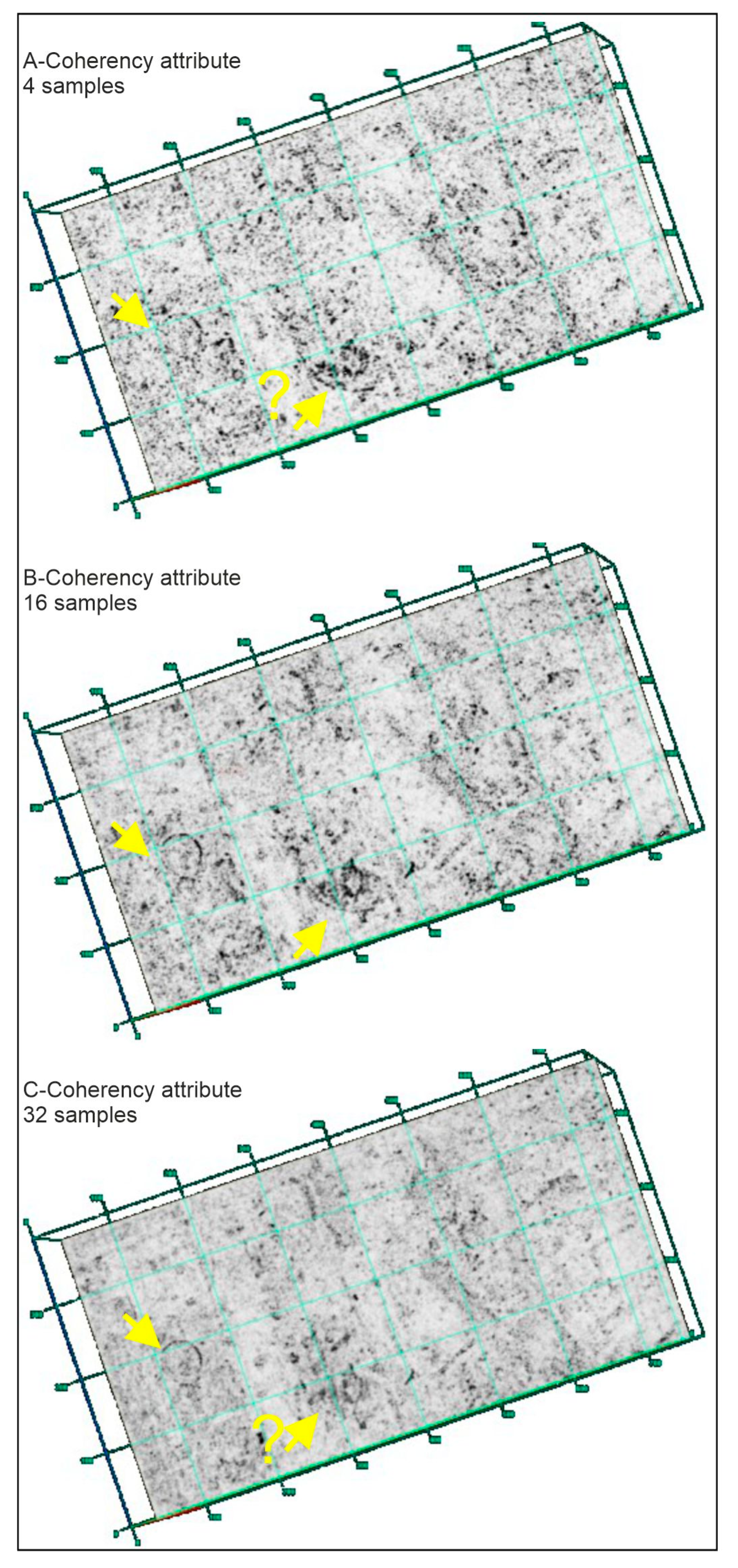
- Trinks, I.; Hinterleitner, A. Beyond Amplitudes: Multi-Trace Coherence Analysis for Ground-Penetrating Radar Data Imaging. Remote Sens. 2020, 12, 1583. [Google Scholar] [CrossRef]
- Verdonck, L. Detection of Buried Roman Wall Remains in Ground-penetrating Radar Data using Template Matching. Archaeol. Prospect. 2016, 23, 257–272. [Google Scholar] [CrossRef]
- Verdonck, L.; Taelman, D.; Vermeulen, F.; Docter, R. The Impact of Spatial Sampling and Migration on the Interpretation of Complex Archaeological Ground-penetrating Radar Data. Archaeol. Prospect. 2015, 22, 91–103. [Google Scholar] [CrossRef]
- Schmidt, A.; Dabas, M.; Sarris, A. Dreaming of Perfect Data: Characterizing Noise in Archaeo-Geophysical Measurements. Geosciences 2020, 10, 382. [Google Scholar] [CrossRef]
- Bahorich, M.S.; Farmer, S.L. 3-D seismic coherency for faults and stratigraphic features. Lead. Edge 1995, 14, 1053–1058. [Google Scholar] [CrossRef]
- Forte, E.; Pipan, M.; Casabianca, D.; Di Cuia, R.; Riva, A. Imaging and characterization of a carbonate hydrocarbon reservoir analogue using GPR attributes. J. Appl. Geophys. 2012, 81, 76–87. [Google Scholar] [CrossRef]


Publisher’s Note: MDPI stays neutral with regard to jurisdictional claims in published maps and institutional affiliations. |
© 2021 by the authors. Licensee MDPI, Basel, Switzerland. This article is an open access article distributed under the terms and conditions of the Creative Commons Attribution (CC BY) license (https://creativecommons.org/licenses/by/4.0/).
Share and Cite
Forte, E.; Mocnik, A.; Basso, P.; Casagrande, G.; Martinucci, D.; Pillon, S.; Possamai, M.; Zambrini, R. Optimised Extraction of Archaeological Features from Full 3-D GPR Data. Appl. Sci. 2021, 11, 8517. https://doi.org/10.3390/app11188517
Forte E, Mocnik A, Basso P, Casagrande G, Martinucci D, Pillon S, Possamai M, Zambrini R. Optimised Extraction of Archaeological Features from Full 3-D GPR Data. Applied Sciences. 2021; 11(18):8517. https://doi.org/10.3390/app11188517
Chicago/Turabian StyleForte, Emanuele, Arianna Mocnik, Patrizia Basso, Giulia Casagrande, Davide Martinucci, Simone Pillon, Marco Possamai, and Roberta Zambrini. 2021. "Optimised Extraction of Archaeological Features from Full 3-D GPR Data" Applied Sciences 11, no. 18: 8517. https://doi.org/10.3390/app11188517