Through-Life Maintenance Cost of Digital Avionics


1
Projects and Maintenance Section, The Private Department of the President of the United Arab Emirates, Abu Dhabi 000372, UAE
2
Department of Electronics, Robotics, Monitoring and IoT Technologies, National Aviation University, 03058 Kyiv, Ukraine
*
Author to whom correspondence should be addressed.
Appl. Sci. 2021, 11(2), 715; https://doi.org/10.3390/app11020715
Submission received: 14 November 2020
/
Revised: 7 January 2021
/
Accepted: 10 January 2021
/
Published: 13 January 2021
(This article belongs to the Special Issue Aerospace System Analysis and Optimization)
Abstract
:Modern avionics can account for around 30% of the total cost of the aircraft. Therefore, it is essential to reduce the operational cost of avionics during a lifetime. This article addresses the critical scientific problem of creating the appropriate maintenance models for digital avionics systems that significantly increase their operational effectiveness. In this research, we propose the lifecycle cost equations to select the best option for the maintenance of digital avionics. The proposed cost equations consider permanent failures, intermittent faults, and false-positives occurred during the flight. The lifecycle cost equations are determined for the warranty and the post-warranty interval of aircraft operation. We model several maintenance options for each period of service. The cost equations consider the characteristics of the permanent failures and intermittent faults, conditional probabilities of in-flight false-positive and true-positive as well as the cost of different maintenance operations, duration of the flight, and some other parameters. We have demonstrated that a three-level post-warranty maintenance variant with a detector of intermittent faults is the best because it minimizes the total expected maintenance cost several folds compared to other maintenance options.
1. Introduction
Modern avionics comprises redundant electronic systems. Each such system may contain two or three identical line replaceable units (LRU). Each LRU operates to a safe failure, which is recorded in-flight or after landing. Since LRU is recovered after a failure, this maintenance strategy is called run-to-failure. The choice of the implementation of the maintenance of avionics systems largely determines the aircraft operation’s efficiency. After the start of its service, the entire life cycle of the aircraft can divide into two stages: warranty and post-warranty period. It is desirable for each period to select the optimal maintenance option, thus minimizing the maintenance cost over the life cycle. If the airline buys a new plane, it is necessary to choose a warranty service option and assess the possible fines imposed on the supplier if the warranty is not complied with. One of the most critical tasks that must be performed when purchasing a new aircraft is to prove the warranty service’s reasonableness and evaluate the buyer’s cost upon the warranty period. During the operation period after the warranty, the aircraft owner pays all maintenance costs. Modern avionics systems are characterized by a high level of testability and maintainability. Shop replaceable units (SRU) are the interchangeable components of an LRU. An SRU is generally a printed circuit board assembly that can be replaced at a backstop. Modern electronic LRU usually has built-in test equipment (BITE) for in-flight testing. The described design of avionics systems gave rise to the following three levels of maintenance: organizational maintenance (O-level), intermediate maintenance (I-level), and depot maintenance (D-level). LRU rejected in-flight is dismantled from aircraft and then serviced at the O-Level, also called a flight line maintenance. Specialized backshops located at the airline base usually conduct maintenance at the I-level. I-level support is more particularized, allowing testing and recovering rejected units at the O-level. The repairing of the faulty LRU at the I-level is carried out by replacing the defective SRU. Consequently, the spare parts at the I-level are SRU. D-level maintenance provides the repair of SRU rejected at the I-level. The spare parts at this maintenance level are electrical and electronic components. At present, some airlines eliminate D-level and occasionally even I-level maintenance by outsourcing the heavy work to repair stations. Major US airlines often use outsourced repair stations, with about 24% of heavy aircraft servicing done outside the US [1]. However, American Airlines, one of the country’s largest airlines, fulfills most of the support internally. Therefore, there are many options for using one-, two-, or three-level systems to service avionics. We need to have an objective function for comparing alternatives among possible maintenance options. The objective function can be a maintenance cost, considering the essential technical characteristics. Avionics failures cause many situations like “aircraft on the ground”, which lead to significant economic losses [2]. Therefore, the maintenance cost function should include characteristics of operational reliability. A study by the FAA found that flight delays in 2007 cost airlines an estimated $31 billion [3]. Permanent failures and intermittent faults represent most of the avionics refusals. The major causes of unconfirmed failures in civil and military aviation are intermittent faults and false alarms. We should note that intermittent faults and false alarms are a significant root of so-called no fault found (NFF) occasions in onboard electronic systems. In avionics, the estimated level of NFF is 20% to 50% [4,5], leading to about 27% of unscheduled removals of avionics LRU [6]. The aviation industry’s false alarm rate is very high, achieving 28% of all incidents related to alarms [7]. Intermittent faults and false alarms directly impact avionics maintenance costs because of the increased downtime, violated regularity of flights, increased number of spare LRU, etc. We should also note that in military avionics the situation with NFF is even worse. According to [8], in the Turkish Air Force, the overall percentage of NFF is 45%, with a distribution of NFF 47.6% for digital and 63% for analog LRU.
From the literature review (Section 2), we can conclude that published studies do not examine the combined effect of permanent failures, intermittent faults, and false-positives on onboard electronic systems’ maintenance cost. We direct this study on the development of life cycle cost equations that allow airlines to choose the optimal service option from several practically implementable choices. The proposed cost equations consider the impact of permanent failures, intermittent faults, in-flight false-positives, average flight duration, maintainability of LRU, quantity of spare parts in the warehouse, the presence of automated test equipment (ATE), and the fault (or failure) location depth of faulty LRU at I- and D-level. We derive the mathematical equation for the meantime between unscheduled removals (MTBUR) and analyze maintenance options with one, two, and three levels. We determine the quantity of spare LRU that minimizes aircraft delays. We also analyze the dependence of the optimal quantity of LRU in the warehouse regarding the probability of BITE false-positive and rate of intermittent faults. We determine the objective cost functions required to select the optimum variant for servicing avionics singly for the warranty and post-warranty time-intervals since they have varied cost components.
The article has the following organization: Section 2 provides a review in the field of modeling avionics maintenance. In Section 3, we describe the proposed mathematical model of avionics maintenance. Section 4 and Section 5 consider warranty and post-warranty maintenance models of avionics systems, respectively. Section 6 consider minimizing the expected maintenance cost of avionics systems during service life. In Section 7, we present the results and discussion. In Section 8, we formulate the conclusions. Appendix A, abbreviations, nomenclature, and references are given at the end of the article.
2. Review
Evaluation of the cost of avionics maintenance has been conducted in many studies. Feldman et al. [9] considered a mathematical model for calculating the cost of servicing one LRU socket on the plane. The authors used stochastic simulation modeling to determine the parameters included in the proposed model. Scanff et al. [10] proposed a simulation model to compare helicopter avionics systems’ lifecycle cost about various maintenance options, including unscheduled maintenance, fixed-interval scheduled maintenance, and condition-based maintenance. Zerbe et al. [11] applied a model-based design to avionics, considering maintenance and logistics operations and their impact on fleet availability. Dhillon [12] considered a simple cost equation for assessing the maintenance cost of such an avionics system as an air data computer. Jun and Huibin [13] applied the FMECA method, which specifies the maintenance scope and procedure for each aircraft system, to reliability modeling considering the function performed by each part of the system. Wang and Song [14] compared the maintenance systems of dismantled avionics LRU with a different number of levels. The authors proposed a cost function for the transition from a three-level to a two-level maintenance system. Simulation modeling determines each of the cost components. Ulansky and Terentyeva [15] considered a maintenance model of an unceasingly monitored digital electronic system in which revealed, unrevealed and intermittent failures might occur. Safaei [16] proposed a novel methodology to assess the impact of premature maintenance on the total maintenance cost. Saltoglu et al. [17] developed downtime cost models for scheduled airline operators. Each model consists of the cost of owning an aircraft and either subchapter cost or opportunity cost. The proposed models can be applied to different groups of aircraft equipment. Mason [18] developed a model for comparing a two-level and three-level maintenance system of the F-117A stealth fighter avionics. The proposed formulas can only be used to compare two-level and three-level maintenance systems regarding the number of spare LRU. Nakagawa [19] considered a telecommunication system with intermittent faults. The time to a fault has an exponential distribution. Faults become permanent when the unrevealed state duration exceeds the upper time limit. Erkoyuncu et al. [20] considered a consequential model of the primary cost drivers of the aggregated cost of NFF aftermaths. The article shows how to choose the most suitable drivers to represent the total losses corresponding to NFF. The general NFF value pricing framework demonstrates how qualitative and quantitative information can achieve service goals. Cai et al. [21] considered a Bayesian network based on the method for diagnosing transient and intermittent faults. Rashid [22] assessed the effect of various variants of processor recovery after occurring an intermittent fault on its performance. He simulated a fault-tolerant multicore processor at the action of intermittent faults subject to exponential and Weibull distributions. As shown in the study, the processor faults are 40% intermittent and 60% permanent. Ilarslan et al. [23] described some maintenance strategies based on NFF distribution using empirical equations. According to the authors, in military aviation, NFF events account for approximately 70% of all avionics failures. Raza and Ulansky [24,25] developed maintenance models of onboard electronic LRU considering permanent failures and intermittent faults. For calculating the operational reliability indicators, the authors introduced the conditional probabilities of in-flight fault occurrence and non-occurrence. Raza [26] proposed a mathematical model for digital avionics maintenance. The model can be used for any distribution of permanent failures and intermittent faults. Raza and Ulansky [27] considered the mathematical model of decision-making for uninterrupted monitoring of the LRU parameter in-flight. They assessed the cost associated with false alarms and intermittent faults.
Based on the analysis of previously published studies, the following conclusions can be drawn. In the maintenance models presented in studies [9,10,11,12,13,14,16,17], the impact of intermittent faults and in-flight false-positives on the maintenance cost was not considered. The models proposed by Ulansky, Terentyeva, and Nakagawa in [15,19] can be used only for systems with a continuous mode of operation. Onboard electronic systems have a discontinuous operation due to the rotation of flights and landings. Consequently, the models are not acceptable for describing avionics systems. The study [20] shows the relevance of assessing the NFF impact on maintenance cost; however, the authors do not propose mathematical or simulation models. The Markov model developed by Cai et al. [21] may not be used for modeling the intermittent faults in avionics systems since transient faults usually occur in electrical power systems. Ilarslan et al. [23] proposed empirical equations that can only be used with the specified percentage distributions of confirmed and unconfirmed failures. Raza and Ulansky proposed in [24,25,26] avionics maintenance models considering permanent failures and intermittent faults. However, in the studies [24,25], the models require to know the conditional probabilities of in-flight occurrence and non-occurrence of intermittent faults, which are known for exponential time distribution and not easy to derive for any other distribution. The model considered by Raza and Ulansky in [27] is valid only for continuous monitoring with the help of analog sensors. Thus, from the conducted analysis of recently published studies follows that the combined impact of the in-flight false-positives, permanent failures, and intermittent faults on the maintenance cost of digital avionics has not been considered.
3. Mathematical Modeling of Avionics Maintenance
Consider the process of operating and maintaining an LRU in the time interval (0, T). Suppose that the flight duration is τ, and in the interval (0, T) there are M + 1 flights, i.e., T = (M + 1)τ. During any flight, the BITE performs LRU testing, which is imperfect to some degree. Due to imperfection of BITE testing, wrong decisions are possible regarding the condition of LRU. A full group of incompatible events when testing the LRU during flight includes the following: true-positive, false-positive, true-negative, and false-negative. Further, it is assumed that in the LRU during the flight a permanent failure or an intermittent fault may occur. In the case of a permanent failure upon the flight, the onboard computer will disable the LRU or ignore its information. In the case of an intermittent fault in-flight, the LRU usually does not shut down during the flight. Still, the onboard computer will record information about the intermittent fault that occurred during the last flight.
Thus, after aircraft landing, the LRU is demounted from the aircraft board on one of the following occasions:
- -
- the event of a “false-positive” occurred in the last flight,
- -
- the event of a “true-negative” happened during the last flight,
- -
- an intermittent fault occurred in the previous flight.
The expected maintenance cost (EMC) is dependent on the chosen maintenance option for a specific period of the lifetime. The EMC, in general, we calculate as follows:
where q is the quantity of identical LRU on the aircraft board, N is the quantity of aircraft in the fleet of the airline, is the expected cost of repairing the LRU removed from the aircraft board for the maintenance option number i, is the expected number of the unscheduled LRU removals during time T, is the capital expenditures for the maintenance option number i.
As shown in (1), parameters q, N, and do not depend on the selected maintenance option. Parameters and rely on the maintenance organization and capital expenditures introduced to the diagnostic equipment and spare parts.
First of all, let us determine the . The expected number of the unscheduled LRU removals in the time span (0, T) is the ratio of T to the MTBUR, i.e.,
where is the MTBUR on a finite time horison (0, T).
MTBUR is one of the essential indicators of avionics operational reliability. This indicator depends on the characteristics of the LRU permanent failure-free and intermittent fault-free operation and the validity of the in-flight BITE functioning. Under [28], the MTBUR is about 50% of the MTBF for modern avionics, where MTBF is the mean time between permanent failures. This difference between MTBUR and MTBF leads to increased direct operating costs of about 40% [29].
Let’s determine an equation for MTBUR considering the main causes of LRU dismounting from the aircraft board, including failures, faults, and the false-positives of BITE during the flight. Let the permanent failure arises at the time H = η, where , and H is the random time to permanent failure. Consider the events leading to the unscheduled LRU removal from the aircraft board. If a false-positive occurs during the ν-th flight the LRU will operate till the time ντ, where . By the formula of mathematical expectation for a discrete random variable, we determine that
where is the conditional mathematical expectation of the time to unscheduled removal due to false-positive, is the conditional probability of false-positive during ν-th flight provided that H = η, and Ω(t) is the cumulative distribution function (CDF) of the time to intermittent fault.
Besides, the LRU will be removed at time lτ if during the l-th flight an intermittent fault occurs, where . By the formula of mathematical expectation for a discrete random variable, we obtain
where is the conditional mathematical expectation of the time to unscheduled removal due to intermittent fault, is the conditional probability of true-positive during l-th flight provided that H = η, and ω(t) is the probability density function (PDF) of the time to intermittent fault.
Finally, if there was no BITE error like false-positive or intermittent fault before the moment , then the LRU will be dismantled after the aircraft landing at the moment . In this case, the expected time till LRU removal is given by
Now assume that . In this case, the following formulas determine the conditional mathematical expectation of the time to unscheduled removal:
- due to false-positive
- due to intermittent fault
- due to permanent failure:
Thus, assuming that H = η and considering (3)–(8), the expected time between unscheduled LRU removals is
We define the conditional probability as the probability of mutual occurrence of the following events: when tested during flights, BITE judged the LRU as operable, and during the -th flight BITE recognized the LRU as inoperable, provided that H = η. Analogically, the conditional probability presents the probability of mutual occurrence of the following events: when tested during flights, BITE judged the LRU as operable, provided that H = η.
We determine MTBUR by the formula of total expectation of continuous random variable, which is random time to permanent failure
where f(η) is the PDF of the time to permanent failure.
Substituting (9) to (10) gives
In (11), to calculate the MTBUR, it is needful to have information about the in-flight false-positive and true-positive probabilities and the PDF of the time to permanent failure and intermittent fault.
According to [30], the exponential distribution is suitable to describe the failure distribution of complicated technical equipment. Onboard electronic systems have a complex structure and include a considerable quantity of electronic elements. The influence of external and internal mechanisms on the electronic components may lead to LRU failure. Various failure mechanisms can add up, leading to a constant failure rate, which is possible only with an exponential law of distribution of the operating time to failure [31].
Let’s determine MTBUR for the exponential failure and fault distribution with the following PDF and CDF:
where λ and θ are, respectively, permanent failure and intermittent fault rate.
Under the memoryless property of the exponential distribution of the time to permanent failure, the conditional probabilities and do not depend on the time to failure. Therefore, as shown in the study [32] (p. 89), the conditional probabilities of false-positive and true-positive can be presented in the following form:
where is the conditional probability of a false-positive event during flight.
In-flight, digital avionics systems can be in one of two modes: operation and testing. In operation mode, each avionics system performs its intended functions. In the testing mode, the avionics system does not operate because of performing self-testing. Let us consider example of a Very High-Frequency Omni-Directional Range (VOR) radio navigation system. In the testing mode, a simulated beacon signal with a given azimuth value is generated in an onboard VOR receiver. Then, this signal is fed to the antenna input of the VOR receiver for processing in the same way as the working signal in the operation mode. The decision on the operability of the VOR receiver measuring path is made by comparing the measured value of the tested parameter with the specified one. The test parameter for the VOR receiver is the azimuth measurement error. The time between in-flight test checks is significantly higher than the transient time in corresponding systems, so such checks can be considered independent.
Assume there are n test checks during the flight and permanent failures have an exponential distribution. Besides, the conditional probability of false-positive for a single checking the system by BITE is α. Then, as shown in the study [32] (p. 90), the following formulas calculate the conditional probabilities of false-positive and true-positive:
Let’s simplify the equation for MTBUR by substituting (12)–(16) to (11).
Taking all finite series in (19) and performing required integration, we obtain Equation (A1) (see Appendix A). Equation (A1) is rather cumbersome; however, when using it, calculation of MTBUR requires much less time compared to computing (19).
4. Warranty Maintenance Models of Avionics Systems
Correct regulation of the relationship between the supplier (manufacturer) of the aircraft and the buyer (airline) primarily determines its efficiency in operation. The most acute problem faced in this relationship arises during the warranty period when the supplier bears the main costs of repairing the aircraft systems. The supplier fixes the system’s defect by free charge and can either replace or repair the failed system within a reasonable time. However, the buyer must acquire sufficient spare LRU to guarantee the absence of flight delays. The quantity of spare LRU is dependent on the chosen option of warranty maintenance (WM). For avionics systems, the selection of the optimal WM option is dependent on the following: (a) supplier’s warranty obligations; (b) operational reliability indexes; c) whether the buyer has ground test equipment [33] (p. 86).
Manufacturers and suppliers of avionics systems typically use the following warranty time-related indicators: warranty period (TW), guaranteed repair time (TRS), and guaranteed expedited delivery time of a spare LRU (TED). Warranty time-related indicators have specific units of measurement. The warranty period is expressed in a calendar period (years, months) from the beginning of the warranty. The guaranteed turnaround time on a repair is computed in a calendar duration (days) from the beginning of repair. The guaranteed expedited delivery time of a spare LRU is expressed in a calendar duration (days) from the claim date. Any contract for the supply of avionics systems specifies the values of TW, TRS, and TED.
The supplier’s time-related indicators of the warranty may be presented in different measurement units. For instance, assume that TW = 2 years and the yearly aircraft flight time is 2500 h; then, if necessary, we can measure the warranty period in hours, e.g., TW = 2 × 2500 = 5000 h. Sometimes, the warranty period’s length is specified separately in the calendar duration and flight hours. In such cases, the TW indicator equals the value that is reached first.
The aircraft buyer does not pay for repairing the failed LRU during the warranty period. However, it pays for spare units needed to guarantee flight regularity. Consequently, the aircraft buyer should select a WM option corresponding to the minimum total operating costs. Various WM options may depend on whether the airline has ground test equipment and TRS and TED values. The existence of ground test equipment at the airline base allows testing the operability of the dismounted LRU and shipping only those LRU to the manufacturer that have confirmed failures. Airline sends the LRU whose failures were not confirmed to the warehouse. Such LRU are included in the exchange fund and can be installed onboard upon request.
The first WM option includes only O-level maintenance. Here, all LRU, rejected by BITE, the airline ships to the manufacturer for repair. The most significant cost indicator for the airline during the warranty period is the total expected maintenance cost, which we denote by EMCW. It is clear that during warranty, EMCW comprises the cost of dismounting and installing the LRU on the aircraft board and the cost of LRU in the warehouse recalculated per one aircraft.
We denote the average costs associated with the first WM option as . Evident that the cost of spare LRU has a significant impact on .
We determine by the following formula:
where q is the quantity of the same LRU in the onboard electronic system, LC is the operational maintenance labor cost per hour ($/h), is the mean time of O-level maintenance, is the average number of unscheduled removals of LRU due to permanent failures, intermittent faults, and in-flight false-positives for time , is the quantity of airplanes under the supplier’s warranty, PS is the planned quantity of spare LRU in the warehouse, US is the unplanned quantity of spare LRU that will need to be supplied from the manufacturer to provide flight regularity, and is the cost of a spare LRU.
We assume that the airline has ground test equipment at the I-level maintenance for rechecking the LRU demounted from the aircraft board in the second WM option. Since conventional test equipment cannot practically detect the presence of intermittent faults in dismounted LRU, such units are sent to the warehouse after testing. We denote the average cost associated with the second WM option as . It includes the cost components due to dismounting and installing LRU on aircraft board, rechecking dismounted LRU by ground test equipment, ground test equipment cost, and cost of spare LRU in the warehouse recalculated per aircraft.
The following formula determines :
where is the average LRU testing time at the maintenance on the I-level, is the quantity of different LRU types that the ground test equipment can test at the maintenance on the I-level, is the ground test equipment cost on the I-level.
We can see from (20) and (21) that and depend on the quantities of spare LRU PS and US. Further, we will compute the optimal quantity of spare LRU by using the following criterion [24]:
where is the average waiting time for a spare LRU from the warehouse in the situation “aircraft on the ground”, is the average time of the scheduled stop of the aircraft at the airport of the airline’s base.
We can see from (22) that if , then no disruption of the regularity of flights will occur. In contrast, if , there will be a disruption of the flight regularity. Therefore, the optimal quantity of spare LRU is the minimum possible number of units, which ensures that there are no delays in departures from the airline base airport.
We used the continuous-time Markov chain to describe the operation of the warehouse of spare LRU at the airline base [25].
Let’s evaluate the mean time of LRU repair . For the first WM option, we have
For the second WM option, only those LRUs are shipped to the manufacturer for repair, the permanent failure of which is confirmed by checking using ground test equipment. Therefore, the time will be less than for the first WM option. We compute the time by the formula for a discrete random variable’s mathematical expectation.
where , , and are, respectively, posterior probabilities that the LRU dismounted from the aircraft due to permanent failure, a false-positive error of BITE, or intermittent fault, , , and are, respectively, the time of testing the LRU removed from aircraft due to permanent failure, a false-positive error of BITE, and intermittent fault, and
The sum of the posterior probabilities , , and is equal to one.
We determine the probabilities , , and from Equation (11) by the following formulas:
Substituting (12)–(16) into formulas (26)–(28), we obtain the posterior probabilities for the exponential distributions presented by the PDF (12) and (13).
Taking all finite series in (29)–(31) and performing required integration, we obtain Equations (A2)–(A4) (see Appendix A).
Optimal WM option should ensure the minimum value of the average buyer’s cost during the warranty period, i.e.,
where is the minimal EMCW corresponding to the optimal WM option.
5. Post-Warranty Maintenance Models of Avionics Systems
Low-cost airlines with few aircraft may not have enough money to perform all maintenance levels. Accordingly, these airlines may remove the second and third maintenance levels and use only O-level. In this case, the airline transfers to specialized companies heavy maintenance checks and routines. Such companies are usually called repair stations. According to [34], U.S. airlines outsourced 71% of heavy maintenance in 2008. Therefore, we consider only the organizational level maintenance (O-level) for the first post-warranty maintenance (PWM) option. The first PWM option is simple for airlines but may turn to be very expensive. All LRU that rejected by BITE in-flight the airline should ship to the manufacturer for repair. In this case, for ensuring the flights’ regularity, the airline should buy a comparably large quantity of spare LRU. The first PWM option implies that LRU shipped to the manufacturer will include not only LRU with permanent failures but also LRU removed from airplanes due to intermittent faults and in-flight false-positives. Thus, the airline will have to pay for repairing all LRU dismounted from the aircraft fleet due to permanent failures, intermittent faults and BITE false-positives. Upon expiration of the warranty period, the airline is obliged to pay the cost of repairing the LRU, transportation costs, labor costs, and the cost of the spare LRU. Therefore, the integral maintenance cost indicator for the airline is the total expected maintenance cost during the post-warranty service life of the avionics system, which we denote as EMCPW. This cost comprises the following components for the first PWM option: the cost of dismounting and mounting LRU in the aircraft during the post-warranty period, the cost of delivering LRU to the manufacturer and back to the airline, the cost of LRU repairs, and the cost of spare LRU per aircraft. We determine EMCPW for the first option as follows:
where is the mean cost of LRU shipping to manufacturer and back to the airline, , , and are the mean cost of the LRU repair due to permanent failure, intermittent fault, and in-flight false-positive at the manufacturer, respectively, is the post-warranty period measured in-flight hours, is the average number of unscheduled removals of LRU due to permanent failures, intermittent faults, and in-flight false-positives for time TPW, and is the quantity of aircraft operated in the airline without a warranty.
For the first PWM option the average LRU repair time is calculated by Equation (23).
Let’s consider three different PWM options of the maintenance system with two levels (O- and I-level). For rechecking the dismounted LRU in the first option, the airline uses ground test equipment at the I-level of maintenance. After rechecking, the airline ships the LRU with confirmed failures to the manufacturer or to the outsourcing company for repair. The units with unconfirmed failures are shipped to the warehouse where spare LRU are stored. For this maintenance option, EMCPW includes the following cost components: the cost of O-level maintenance during the time TW, the cost of checking LRU with ground test equipment, the cost of shipping failed LRU to the manufacturer and back, the repair cost of LRU having a permanent failure at the facilities of the manufacturer, the cost of ground test equipment recalculated per one aircraft, and the spare LRU quantity cost recalculated per one aircraft.
We determine EMCPW for the second option as follows:
For the second PWM option the average LRU repair time is calculated by Equation (24).
In the third maintenance option of the two-level system, the I-level uses a ground ATE to recheck the dismounted LRU and detect the failure location with depth to the faulty SRU. As is well-known [35], conventional ATE is not capable of detecting intermittent faults. Therefore, dismounted LRU with intermittent faults and units removed due to in-flight false-positives of BITE after rechecking by ATE will be delivered to the warehouse of spare LRU. Repair of LRU with permanent failures is carried out by replacing the faulty SRU. After identifying the defective SRU, they are delivered to the outsourcing company or manufacturer for repair. Therefore, EMCPW includes the following constituent elements: the cost of O-level maintenance during time TW, the cost of checking the dismounted LRU using ATE and detection of the faulty SRU, the cost of shipping the faulty SRU to the outsourcing company or manufacturer, as well as the repaired SRU back to the airline, the cost of repairing faulty SRU at the outsourcing company or manufacturer, and the cost of ATE and spare LRU and SRU recalculated per one aircraft.
We determine EMCPW for the third option as follows:
where is the mean time of checking the LRU with help of ATE at the I-level, is the mean cost of SRU repair with permanent failure at the outsourcing company or manufacturer, is the mean time to detect the place of a permanent failure in the failed LRU with depth to SRU using ATE, is the mean cost of delivering the faulty SRU to the outsourcing company or manufacturer and back to the airline’s warehouse, is the cost of ATE that serves the I-level, is the quantity of LRU types that ATE can check, is the j-th type SRU cost , is the quantity of spare j-th type SRU, and n is the quantity of SRU types in the examined LRU.
For the third PWM option the average LRU repair time we calculate as follows:
The number of spare SRU we can calculate from the condition of guaranteed provision of all LRU (onboard and spare) with spare SRU at a high probability (0.95–0.99) [36]. In the case when the flow of failures is the homogeneous Poisson point process, we determine the optimum quantity of spare SRU of the j-th type by the Poisson formula as the minimal number satisfying the next condition [36]:
where is the aggregated quantity of the j-th type SRU that installed in all aircraft’ LRU of the airline fleet and spare LRU located in the warehouse, is the probability that the total number of LRU will be provided with SRU type j, is the rate of permanent failures of j-th type SRU, and is the average repair time of the j-th type SRU at the manufacturer.
Conventional ATE may not be used to test intermittent faults for the following reasons [35]: ATE does not check simultaneously all circuits or functional paths of the LRU, including all connection paths to SRU, ATE do not test the LRU in the appropriate operating environment, and ATE are incapable of detecting short-duration intermittent faults that cause NFF. Given the conventional ATE disadvantages, as stated above, specific specialized tools for intermittent fault diagnostics are currently in development. For instance, Universal Synaptics Corporation (USA) produces a Voyager Intermittent Fault Detector (IFD) [37] and an Intermittent Fault Detection and Isolation System (IFDS) [38].
Therefore, in the third variant of the maintenance system with O- and I-level, both ATE and IFD are used at the I-level to check the LRU and detect faulty SRU. The combination of ATE and IFD allows checking the dismounted LRU for permanent failures and intermittent faults and detecting faulty SRU. The repair of LRU is performed by replacing the identified faulty SRU. Further, the airline will ship the SRU with detected defects to the outsourcing company or manufacturer for repair. We should note that IFD can also be used to detect intermittent faults in SRU with the depth up to non-repairable elements.
The expected maintenance cost for this PWM option comprises the same cost components as for the last variant, as well as the additional cost of IFD and operations to detect SRU with intermittent faults. We determine EMCPW by the following formula:
where is the mean cost of repairing the SRU, because of detected intermittency, at the outsourcing company or manufacturer, is the mean time of detecting the place of an intermittent fault in the dismounted LRU with depth to SRU using IFD, is the IFD cost, and is the quantity of LRU types in which IFD can detect intermittent faults.
For the fourth PWM option the average LRU repair time we calculate as follows:
Analogically to (37), by satisfying the following condition, we determine the optimum quantity of the j-th type spare SRU:
where is the intermittent fault rate of the j-th type SRU.
We remind you that level D maintenance is possible to implement if a repair shop has diagnostic equipment for detecting the place of failures and faults in printed circuit boards judged as faulty at the I-level. Maintenance at level D will operate successfully if the warehouse provides the repair shop with spare electronic components. The expected maintenance cost of this PWM option comprises the following constituent elements: the cost of dismounting and mounting the LRU onboard the airplane within the time-interval TW concerning O-level maintenance, the cost of checking the dismounted LRU and identification of faulty SRU by ATE concerning I-level maintenance, the cost of troubleshooting and repairing SRU concerning D-level maintenance, the cost of ATE, IFD, spare LRU, SRU, electrical and electronic elements recalculated per one aircraft.
We determine EMCPW for the three-level maintenance system by the following formula:
where is the mean time to detect the place of a permanent failure with depth to one or more non-repairable electronic components in the SRU and replace them at the D-level maintenance, is the mean time to detect the place of intermittency in the SRU with depth to one or more non-repairable electronic components and replace them at the maintenance on the D-level, is the mean cost of replaced electronic components when repairing the SRU with a permanent failure at the maintenance on the D-level, is the mean cost of replaced electronic components when repairing the SRU with detected intermittency on the D-level, is the cost of equipment used for troubleshooting on D-level, is the quantity of SRU types that the D-level can repair, is the cost of a spare electronic component of the z-th type in the SRU with number y, and is the quantity of spare electronic components of the z-th type in the SRU with number y.
For the fifth PWM option the average LRU repair time is calculated by Equation (39).
Since the fifth PWM option involves D-level for repairing defective SRU and not shipping them to the manufacturer for repair, we determine the optimal number of spare SRU from the following inequality:
The optimal PWM option should satisfy the following criterion:
where is the minimal EMCPW corresponding to the optimal PWM option.
6. Minimizing the Expected Maintenance Cost of Avionics Systems during Service Life
Let’s consider the task of determining the minimum cost of maintenance for a redundant avionics system over its service life. The service life of any technical device is the period from the beginning of its operation to the point of discard. We denote the avionics system service life as . Obviously, the service life includes the warranty and post-warranty periods. Therefore, can be defined in the following form:
In Section 4 and Section 5, we analyzed two WM and five PWM options. In this way, theoretically, ten different combinations of maintenance options can be obtained for the entire service life. Obviously that we can determine the minimum cost of maintenance during service life by solving the following problem:
where is the minimal value of the maintenance cost during service life.
7. Results and Discussion
Section 7.1 and Section 7.2 provide a numerical and graphical analysis of the indicators and characteristics introduced in the previous sections. Wherein a wide range of parameters is used to determine the nature of the behavior of indicators and establish the boundary values of parameters, the excess of which leads to adverse consequences in practice. Section 7.3 calculates all the parameters and indicators necessary to select the optimal maintenance option for the airborne inertial reference system of the A380 aircraft, based on real data.
7.1. Warranty Maintenance
Figure 1 shows the dependency of MTBUR on the in-flight conditional probability of a false-positive computed by Equation (A1) when , , , and .
As we can see in Figure 1, the dependence of MTBUR on can be conditionally divided into three intervals. On the interval from 0 to , MTBUR is practically independent of . When changes from to MTBUR weakly depends on the conditional probability of false-positive during flight and falls by 10%. On the interval from to , MTBUR strongly depends on and decreases by eight times. As it follows from the analysis, the conditional probability of a false positive in-flight should be, at best, less than , or at least no more than for the given data.
Figure 2 shows the dependency of the in-flight conditional probability of a false-positive on the number of in-flight test checks calculated by Equation (17) when . We can conclude from Figure 2 that to provide the in-flight conditional probability of a false-positive in the interval –, the number of in-flight test checks should be 10 to 100.
Let’s calculate the optimal quantity of spare LRU in the airline’s warehouse with the given initial data: , , , , , , , , and .
Figure 3a shows the dependency of the mean waiting time on the number of planned spare LRU (PS) for the first WM option at . Four spare LRU are required for and five spare LRU for to provide the mean waiting time for a spare LRU not exceeding 0.5 h.
Figure 3b shows the same dependency as in Figure 3a but with different rate of intermittent faults and . As we can see in Figure 3b, four spare LRU are required for and seven spare LRU for to provide the mean waiting time for a spare LRU not exceeding 0.5 h.
As we can see in Figure 3a,b, the mean waiting time significantly depends on the conditional probability of in-flight false-positive and the rate of intermittent faults.
Figure 4a shows the dependency of the optimal quantity of spare LRU on the quantity of aircraft for the WM option number one when (red circles), (black squares) and .
Analysis of Figure 4a allows us to draw the following conclusions: the dependency of on is an integer increasing function, a rise in the conditional probability of in-flight false-positive from to results in a substantial increment of the quantity of spare LRU (PS), and a larger increment in the quantity of spare LRU corresponds to a larger value of the probability. The latter circumstance indicates that a high conditional probability of in-flight false-positive has a significant impact on the effectiveness of the first WM option.
Figure 4b illustrates the dependency of the optimal quantity of spare LRU on the quantity of aircraft for the WM option number one when (red circles), (black squares) and . As we can see in Figure 4b, a rise in the rate of intermittent faults results in a significant rise in the quantity of spare LRU. Moreover, the influence of intermittent faults is even more considerable than in-flight false-positives.
Figure 5a,b show the dependency of the expected unplanned quantity of spare LRU (US) on the planned quantity of spare LRU (PS) for the first WM option. As seen, the US decreases rapidly as PS increases. Besides, the US highly depends on the intermittent fault rate (), in-flight conditional probability of a false-positive (), and expedited delivery time (). With an increase of and and a decrease of , US decreases as well.
Let’s analyze the dependences of the posterior probabilities of dismantling the LRU on the conditional probability of in-flight false-positive, rate of intermittent faults and permanent failures. We calculated the plots in Figure 6, Figure 7 and Figure 8 by using Equations (A2)–(A4).
Figure 6 shows the dependences of the posterior probabilities of dismantling the LRU due to the in-flight false-positive (red curve), intermittent fault (black curve), and permanent failure (blue curve) on the conditional probability of in-flight false-positive when , , and . Figure 6a corresponds to the case when and Figure 6b—. As we can see in Figure 6a,b, the probabilities (blue curve) and (black curve) decrease, and the probability (red curve) increases with the rise in the conditional probability of in-flight false-positive. Moreover, the impact of in-flight false-positives increases at a lower intermittent fault rate.
Figure 7 shows the dependences of the posterior probabilities of dismantling the LRU due to the in-flight false-positive (red curve), intermittent fault (black curve), and permanent failure (blue curve) on the intermittent fault rate. The initial data are the same as in Figure 6.
We can see in Figure 7 that the posterior probabilities (red curve) and (blue curve) decrease, and the probability (black curve) increases with the rise in the rate of intermittent faults. We should note that the conditional probability does note have big impact on the probability but it has strong influence on the probabilities and .
Figure 8 shows the dependences of the posterior probabilities of dismounting the LRU due to the in-flight false-positive (red curve), intermittent fault (black curve), and permanent failure (blue curve) on the rate of permanent failures. The initial data are the same as in Figure 6. As we can see in Figure 8, the posterior probabilities (red curve) and (black curve) decrease, and the probability (blue curve) increases with the rise in the rate of permanent failures.
In general, analyzing Figure 6, Figure 7 and Figure 8, we can state that an increase in the conditional probability of in-flight false-positive, or the rate of intermittent faults or permanent failures leads to the rise of corresponding a posterior probability and decrease of two other a posterior probabilities.
Figure 9 shows the dependences of the mean waiting time on the number of spare LRU (PS) for the second WM option when , , , (red circles), (black squares), (red triangles), and the rest of data the same as in Figure 3.
We calculated the mean time of LRU repairing by Equation (24). As we can see in Figure 9a,b, the mean waiting time has a much weaker dependence on the conditional probability of the in-flight false-positive and intermittent fault rate in comparison with the same dependence for the first WM option shown in Figure 3a,b.
Figure 10 shows the dependency of the optimal quantity of spare LRU on the quantity of aircraft for the second WM option when and the rest of data the same as in Figure 4. Figure 10a corresponds to the case when and (red circles), , (black squares), and . We plotted Figure 10b when , (red circles), , (black squares), and .
Comparing the plots in Figure 10a,b, we can observe that the results are different only for . For all other values of , the optimal number of spare LRU is the same. Thus, the optimal amount of spare LRU almost does not depend on the conditional probability of in-flight false-positive and intermittent fault rate. Essentially, the second option is resistant to the negative influence of false-positives and intermittent faults.
7.2. Post-Warranty Maintenance
Let’s calculate the optimal quantity of spare LRU for different PWM options described in Section 5 when h, , , , , , , , and .
Figure 11 and Figure 12 show the dependences of the optimal quantity of planned spare LRU on the quantity of aircraft owned by the airline for the first and second PWM option, respectively.
As we can see in Figure 11, the optimal quantity of spare LRU strongly depends on the conditional probability of in-flight false-positive and intermittent fault rate. Moreover, the dependency of PS on θ (b) is more substantial than on (a).
Figure 12 shows the dependency of the optimal quantity of spare LRU on the quantity of aircraft for the second PWM option. Figure 12a corresponds to the case when and . (red circles), , (black squares), and . Figure 12b matches with , and (red circles), , (black squares), and .
Comparing the graphs in Figure 11 and Figure 12, we state that the optimal quantity of spare LRU is significantly less for the second PWM option than for the first.
Figure 13 shows the dependency of the optimal quantity of spare LRU on the quantity of aircraft for the third PWM option. Figure 13a corresponds to the case when and (red circles), and (black squares), and . Figure 13b meets with and (red circles), and (black squares), and .
As seen in Figure 13a, the optimal quantity of spare LRUs for the third PWM option is independent of the conditional probability of in-flight false-positive for . When , the number of spare LRU for is twice than that for . We should also note that the maximum number of spare LRU for the third PWM option (Figure 13a) is two times less than for the second option (Figure 12a).
Comparing Figure 13a,b, we note that for given flight duration, the rate of intermittent faults has a greater impact on the quantity of spare LRU than the conditional probability of in-flight false-positive.
Figure 14 shows the dependency of the optimal quantity of spare LRU on the quantity of aircraft for the fourth and fifth PWM options. Figure 14a corresponds to the case when and (red circles), and (black squares), and . Figure 14b matches with and (red circles), and (black squares), and . With respect to Figure 14a,b, the same conclusions can be drawn as for Figure 13a,b.
Regarding the dependences of presented in Figure 13a,b and Figure 14a,b, we can observe that the third PWM option is less sensitive to changes in the conditional probability of in-flight false-positive and intermittent fault rate than the fourth and fifth PWM options. Besides, PS = 1 when for the third PWM option (red circles), and PS = 1 only when for the fourth and fifth PWM options; PS = 3 when for the third PWM option (black squares) and for the fourth and fifth PWM options. We explain such behavior of function by the fact that the average repair time is longer for the fourth and fifth than for the third PWM option. This conclusion can be drawn from a comparison of Equations (36) and (39).
7.3. Numerical Example
Let’s consider an example of minimizing the expected cost of warranty maintenance for the A380 airborne inertial reference system (ADIRS). In 2012, the airline Emirates (UAE) received eight aircraft A380 [39]. Each aircraft had three air data inertial reference units (ADIRU) of HG2030BE (Honeywell) type that form the redundant ADIRS system. The reliability characteristics of the HG2030BE ADIRU are as follows: MTBF is 40,000 h, and MTBUR is 23,500 h [40].
ADIRS gives aerial information (airspeed, angle of attack, and altitude) and inertial control information (location and altitude) to pilot display and other aircraft systems such as engines, autopilot, and aircraft chassis. ADIRS comprises three fault-tolerant ADIRU located in the electronic rack of the aircraft. The third ADIRU is a standby unit that may be selected to provide data to the first or second pilot’s displays in the case of a partial or total failure of ADIRU № 1 or № 2. ADIRS does not have crossover redundancy between ADIRU № 1 and ADIRU № 2, since ADIRU № 3 is the only alternative source of air and inertial data. Failure of air data stream from ADIRU № 1 or ADIRU № 2 will result in a loss of airspeed and altitude information on the corresponding display. In any case, the information can only be restored by selecting ADIRU № 3.
According to the data given in [40], the approximate price of ADIRU is $31,000. According to [41], the average flight time (τ) of the A380 is 8 h, and the average flying hours per year for a single A380 is approximately 5000 h. Data on testing and setting up ADIRU in the laboratory are given in [42]. The rest of the initial data are taken from various instructions, technical descriptions and are as follows: , , LC = 15 $, , , , , , and .
Since MTBF = 40,000 h, then . As far as MTBUR is less than MTBF, this decrease is associated with false-positives and intermittent faults. Let’s assume that false-positives and intermittent faults have the same impact on MTBUR. In this case, from Equation (A1) on infinite horizon we numerically find that and .
Table 1 shows the calculated results.
As we can see in Table 1, the expected maintenance costs per aircraft for the first WM option is less than for the second option. Therefore, the first WM option is preferable for the given data.
Let’s consider an example of minimizing the expected cost of post-warranty maintenance for the ADIRS of the aircraft Airbus A380. By September 2017, the Emirates (UAE) airline received 97 A380 aircraft for operation [43]. We determine the average cost per one ADIRS of the A380 for various PWM options by using Equations (33)–(42). According to [44,45], each ADIRU includes the following SRU: an air data computer (ADC), a multi-mode receiver (MMR), three digital ring laser gyros, three quartz accelerometers, and a power supply module. As indicated in [46], the cost of three digital ring laser gyroscopes is about $15,000.
In the calculation of the expected maintenance cost per aircraft for various options of PWM, we used the following data: , , , , , , , , , , , , , , , , , , , , , , , and .
Table 2 shows the results of the calculations.
In the fourth and fifth PWM options, we suppose the use of the IFD, which should reduce the intermittent fault rate in the restored LRU. As stated in [47], the use of IFD in restoring the onboard radars AN/APG-68 operated in F-16, MTBUR raised by more than three-fold. Accordingly, we assumed, in computations related to Table 2, that the intermittent fault rate reduced by a factor of 3, i.e., for the fourth and fifth PWM options.
We calculated the number of spare for P(Hj) = 0.99. The use of inequalities (37), (40), and (42) gives that for the third and fourth PWM options there should be two spare digital ring laser gyros, two spare quartz accelerometers, and one spare ADC, MMR, and power supply each. For the fifth PWM option, the airline should have only one spare unit for each SRU type.
As shown in Table 2, the fifth PWM option has the lowest value of expected maintenance cost and is the best. Indeed, is 11.1 times less than and over 9 times less than . Note also that the use of IFD at I-level maintenance only is inadvisable, since by 15.3%. We should also emphasize that the fifth PWM option requires the least quantity of spare parts, namely two LRU and one SRU of each type.
8. Conclusions
This article has proposed a new mathematical model for assessing the through-life maintenance cost of digital avionics. For the first time, we proposed mathematical equations for evaluating the MTBUR of in-flight monitored avionics systems considering permanent failures, intermittent faults, and false-positives of BITE. It has been shown that the dependence of MTBUR on the conditional probability of in-flight false-positive has a different pattern. At used data, on the interval from 0 to , MTBUR weakly depends on the conditional probability of false-positive during flight and falls maximum by 10%. On the interval from to , MTBUR strongly depends on this probability and decreases by eight times. Therefore, the conditional probability of in-flight false-positive should be at least no more than . It has also been shown that to provide the in-flight conditional probability of a false-positive in the interval –, the number of in-flight test checks should be 10 to 100.
Generalized expected maintenance cost equations during the warranty and post-warranty period of operation of avionics systems, seeing the characteristics of permanent failures, intermittent faults, and in-flight false-positives of BITE, have been developed for various maintenance options that differentiate by the number of maintenance levels, allowing to choose the most effective maintenance option for each maintenance period. Numerical analysis has shown that ATE’s use at the I-level maintenance virtually eliminates the harmful effect of intermittent faults and in-flight false-positives on the quantity of spare LRU. We show that the third PWM option is less sensitive to changes in the conditional probability of in-flight false-positive and the rate of intermittent faults than the fourth and fifth PWM options concerning the number of spare LRU, which is because the mean repair time is longer for the fourth and fifth than for the third PWM option. Considering as an example the avionics system ADIRS installed on A380 (Emirates Airline), we have demonstrated that the maintenance option with three levels provided the use of IFD on the levels I and D is the best. Because it decreases the full expected cost of maintenance by eleven-fold as compared to only I-level maintenance, by nine-fold compared to a two-level choice without IFD, by 1.45 fold in comparison with three-level maintenance without using IFD, and by 1.71 fold compared to the three-level option with IFD only at the I-level.
In future research, we hope to develop the cost models for post-warranty maintenance options involving only outsourcing service companies.
Author Contributions
This article presents the collective work of two authors. The authors (A.R. and V.U.) jointly participated in conceptualizing the problem, formal analysis, development of mathematical models, data curation, numerical calculations, and writing the article. All authors have read and agreed to the published version of the manuscript.
Funding
This research received no external funding.
Institutional Review Board Statement
Not applicable.
Informed Consent Statement
Not applicable.
Data Availability Statement
Data sharing not applicable. No new data were created or analyzed in this study. Data sharing is not applicable to this study.
Conflicts of Interest
The authors declare no conflict of interest.
Nomenclature
| T | finite time horizon |
| τ | flight duration |
| M | number of flights |
| expected maintenance cost for maintenance option number i | |
| q | quantity of identical LRU on the aircraft board |
| N | quantity of aircraft in the airline fleet |
| expected repair cost of LRU removed from the aircraft board for the maintenance option number i | |
| expected number of the unscheduled LRU removals during time T | |
| capital expenditures for the maintenance option number i | |
| MTBUR on a finite time interval (0, T) | |
| η | time of permanent failure occurrence |
| conditional probability of false-positive during ν-th flight provided that permanent failure occurs at time η | |
| conditional probability of true-positive during l-th flight provided that permanent failure occurs at time η | |
| Ω(t) | cumulative distribution function |
| ω(t) | probability density function of the time to intermittent fault |
| H | random time to permanent failure |
| expected time between unscheduled LRU removals provided that H = η | |
| λ | permanent failure rate |
| θ | intermittent fault rate |
| conditional probability of a false-positive event during flight | |
| α | conditional probability of false-positive for a single checking the system by BITE |
| TW | warranty period |
| TRS | guaranteed repair time |
| TED | guaranteed expedited delivery time of a spare LRU |
| expected cost for the first WM option | |
| LC | operational maintenance labor cost per hour |
| mean time of O-level maintenance | |
| average number of unscheduled removals of LRU due to permanent failures, intermittent faults, and in-flight false-positives for time TW | |
| PS | planned quantity of spare LRU in the warehouse |
| US | unplanned quantity of spare LRU that will need to be supplied from the manufacturer to ensure regularity of flights |
| cost of a spare LRU | |
| quantity of airplanes under the supplier’s warranty | |
| expected cost for the second WM option | |
| average LRU testing time using the ground test equipment at the I-level maintenance | |
| quantity of different LRU types that the ground test equipment can test at the maintenance on the I-level | |
| ground test equipment cost on the I-level | |
| average time of waiting for spare LRU from the warehouse in the situation “aircraft on the ground” | |
| average time of the scheduled stop of the aircraft at the airport of the airline’s base | |
| mean time of LRU repair | |
| a posterior probability that the LRU dismounted from the aircraft due to permanent failure | |
| a posterior probability that the LRU dismounted from the aircraft due to a false-positive error of BITE | |
| a posterior probability that the LRU dismounted from the aircraft due to intermittent fault | |
| time of testing the LRU removed from aircraft due to permanent failure | |
| time of testing the LRU removed from aircraft due to a false-positive error of BITE | |
| time of testing the LRU removed from aircraft due to intermittent fault | |
| minimal EMCW corresponding to the optimal WM option | |
| mean cost of LRU shipping to manufacturer and back to the airline | |
| mean cost of the LRU repair due to intermittent fault at the manufacturer | |
| mean cost of the LRU repair due to permanent failure at the manufacturer | |
| mean cost of the LRU repair due to in-flight false-positive at the manufacturer | |
| post-warranty period measured in flight hours | |
| average number of unscheduled removals of LRU due to permanent failures, intermittent faults, and in-flight false-positives for time TPW | |
| quantity of aircraft operated in the airline without a warranty | |
| expected cost for the first PWM option | |
| expected cost for the second PWM option | |
| expected cost for the third PWM option | |
| expected cost for the fourth PWM option | |
| expected cost for the fifth PWM option | |
| mean time of checking the LRU with help of ATE at the I-level | |
| mean cost of SRU repair with permanent failure at the outsourcing company or manufacturer | |
| mean time to detect the place of a permanent failure in the failed LRU with depth to SRU using ATE | |
| mean cost of delivering the faulty SRU to the outsourcing company or manufacturer and back to the airline’s warehouse | |
| cost of ATE that serves the I-level | |
| quantity of LRU types that ATE can check | |
| j-th type SRU cost | |
| n | quantity of SRU types in the examined LRU |
| quantity of spare j-th type SRU | |
| aggregated quantity of the j-th type SRU that installed in all aircraft’ LRU of the airline fleet and spare LRU located in the warehouse | |
| probability that the total number of LRU will be provided with SRU type j | |
| rate of permanent failures of j-th type SRU | |
| average repair time of the j-th type SRU at the manufacturer | |
| mean cost of repairing the SRU, because of detected intermittency, at the outsourcing company or manufacturer | |
| mean time of detecting the place of an intermittent fault in the dismounted LRU with depth to SRU using IFD | |
| IFD cost | |
| number of LRU types that can be tested using IFD to detect intermittent faults | |
| intermittent fault rate of the j-th type SRU | |
| mean time to detect a permanent failure in the SRU with depth to one or more non-repairable electronic components and replace them at the D-level maintenance | |
| mean time to detect an intermittent fault in the SRU with depth to one or more non-repairable electronic components and replace them at the D-level maintenance | |
| mean cost of replaced electronic components when repairing the SRU with a permanent failure at the maintenance on the D-level | |
| mean cost of replaced electronic components when repairing the SRU with detected intermittency on the D-level | |
| cost of equipment used for troubleshooting on D-level | |
| number of SRU types repaired at the D-level maintenance | |
| cost of a spare electronic component of the z-th type in the SRU with number y | |
| quantity of spare electronic components of the z-th type in the SRU with number y | |
| minimal EMCPW corresponding to the optimal PWM option | |
| minimum value of the expected maintenance cost during service life |
Abbreviations
The following abbreviations exists in the manuscript:
| ADC | air data computer |
| ADIRU | air data inertial reference unit |
| ADIRUS | air data inertial reference system |
| ATE | automated test equipment |
| BITE | built-in test equipment |
| CDF | cumulative distribution function |
| EMC | expected maintenance cost |
| EMCW | expected maintenance cost during the warranty period |
| FMECA | failure mode effect and criticality analysis |
| IFD | intermittent fault detector |
| IFDIS | intermittent fault detection and isolation system |
| LRU | line replaceable unit |
| MMR | multi-mode receiver |
| MTBF | mean time between failures |
| MTBUR | mean time between unscheduled removals |
| NFF | no fault found |
| probability density function | |
| PWM | post-warranty maintenance |
| SRU | shop replaceable unit |
| VOR | very high-frequency omni-directional range |
| WM | warranty maintenance |
Appendix A
Taking all finite series in (13) and performing required integration, we obtain the following equation:
where and .
Taking all finite series in (23) and (24) and performing required integration, we obtain the posterior probabilities of dismantling the LRU from the aircraft due to permanent failure and a false-positive error of BITE
We find the posterior probability PIF as follows
References
- Reed, T. Amount of Outsourced Offshore Airline Maintenance Work Has Risen, Report Says. Available online: https://www.forbes.com/sites/tedreed/2018/04/06/amount-of-outsourced-offshore-airline-maintenance-work-has-risen-report-says/#6679dda126e2 (accessed on 6 April 2018).
- Seidenman, P.; Spanovich, D. Avionics Integrity. Seeking Solutions for Avionics AOG Angst. Available online: http://aviationweek.com/awin/avionicsintegrity (accessed on 1 September 2011).
- Aircraft on Ground (AOG)—The Causes and Costs of a Grounded Aircraft. Available online: https://www.proponent.com/causes-costs-behind-grounded-aircraft/ (accessed on 26 July 2017).
- Soderholm, P. A system view of the no fault found (NFF) phenomenon. Reliab. Eng. Syst. Saf. 2007, 92, 1–14. [Google Scholar]
- Khan, S.; Phillips, P.; Jennions, I.; Hockley, C. No Fault Found events in maintenance engineering Part 1: Current trends, implications and organizational practices. Reliab. Eng. Syst. Saf. 2014, 123, 183–195. [Google Scholar]
- Hockley, C.; Phillips, P. The impact of no fault found on through-life engineering services. J. Qual. Maint. Eng. 2012, 18, 141–153. [Google Scholar]
- Bliss, J.P. Investigation of alarm-related accidents and incidents in aviation. Int. J. Aviat. Psychol. 2003, 13, 249–268. [Google Scholar]
- Ilarslan, M.; Ungar, L.Y. Mitigating the impact of false alarms and no fault found events in military systems. IEEE Instrum. Meas. Mag. 2016, 19, 16–22. [Google Scholar]
- Feldman, K.; Jazouli, T.; Sandborn, P. A methodology for determining the return on investment associated with prognostics and health management. IEEE Trans. Reliab. 2009, 58, 305–316. [Google Scholar]
- Scanff, E.; Feldman, K.L.; Ghelam, S.; Sandbornb, P.; Gladec, M.; Foucher, B. Life cycle cost impact using prognostic health management (PHM) for helicopter avionics. Microelectron. Reliab. 2007, 47, 1857–1864. [Google Scholar]
- Zerbe, V.; Schulz, M.; Zimmermann, A.; Marwedel, S. Model-based evaluation of avionics maintenance and logistics processes. In Proceedings of the 2010 IEEE International Conference on Systems, Man and Cybernetics, Istanbul, Turkey, 10–13 October 2010. [Google Scholar]
- Dhillon, B.S. Maintainability, Maintenance, and Reliability for Engineers; CRC Press: London, UK, 2006; 278p. [Google Scholar]
- Jun, L.; Huibin, X. Reliability analysis of aircraft equipment based on FMECA method. Phys. Procedia 2012, 25, 1816–1822. [Google Scholar]
- Wang, Y.; Song, B. Manpower management benefits predictor method for aircraft two-level maintenance concept. Mod. Appl. Sci. 2008, 2, 33–37. [Google Scholar]
- Ulansky, V.; Terentyeva, I. Availability modelling of a digital electronic system with intermittent failures and continuous testing. Eng. Lett. 2017, 25, 104–111. [Google Scholar]
- Safaei, N. Premature aircraft maintenance: A matter of cost or risk? IEEE Trans. Syst. Man Cybern. Syst. (Early Access) 2019, 1–11. [Google Scholar]
- Saltoglu, R.; Humaira, N.; İnalha, G. Aircraft scheduled airframe maintenance and downtime integrated cost model. Adv. Oper. Res. 2016, 2016, 1–12. [Google Scholar]
- Mason, R.L. Stealth fighter avionics: 2LM versus 3LM. Air Force J. Logist. 1998, 22, 31–34. [Google Scholar]
- Nakagawa, T. Advanced Reliability Models and Maintenance Policies; Springer: London, UK, 2008; 234p. [Google Scholar]
- Erkoyuncu, S.; Khan, S.; Hussain, S.M.F.; Roy, R. A framework to estimate the cost of no-fault-found events. Int. J. Prod. Econ. 2016, 173, 207–222. [Google Scholar]
- Cai, B.; Liu, Y.; Xie, M. A dynamic-Bayesian-network-based fault diagnosis methodology considering transient and intermittent faults. IEEE Trans. Autom. Sci. Eng. 2017, 14, 276–285. [Google Scholar]
- Rashid, L.; Pattabiraman, K.; Gopalakrishnan, S. Intermittent hardware errors recovery: Modelling and evaluation. In Proceedings of the 2012 Ninth International Conference on Quantitative Evaluation of Systems (QEST), London, UK, 17–20 September 2012. [Google Scholar]
- Ilarslan, M.; Ungar, L.Y.; Ilarslan, K. An economic analysis of false alarms and no fault found events in air vehicles. In Proceedings of the 2016 IEEE AUTOTESTCON, Anaheim, CA, USA, 12–15 September 2016. [Google Scholar]
- Raza, A.; Ulansky, V. Minimizing total lifecycle expected costs of digital avionics’ maintenance. Procedia Cirp 2015, 38, 118–123. [Google Scholar]
- Raza, A.; Ulansky, V. Assessing the impact of intermittent failures on the cost of digital avionics’ maintenance. In Proceedings of the 2016 IEEE Aerospace Conference, Big Sky, MT, USA, 5–12 March 2016. [Google Scholar]
- Raza, A. Maintenance model of digital avionics. Aerospace 2018, 5, 1–16. [Google Scholar]
- Raza, A.; Ulansky, V. Modelling of false alarms and intermittent faults and their impact on the maintenance cost of digital avionics. Procedia Manuf. 2018, 16, 107–114. [Google Scholar]
- Kayton, M.; Friend, W.R. Avionics Navigation Systems, 2nd ed.; John Wiley & Sons Inc.: New York, NY, USA, 1997; p. 700. [Google Scholar]
- Hess, R. Electromagnetic environment. In Digital Avionics Handbook, 3rd ed.; Spitzer, S.R., Ferrell, U., Ferrell, T., Eds.; CRC Press: London, UK, 2017; p. 3. [Google Scholar]
- Drenick, R.F. The failure law of complex equipment. J. Soc. Ind. Appl. Math. 1960, 8, 680–690. [Google Scholar]
- Qin, J.; Huang, B.; Walter, J.; Bernstein, J.; Talmor, M. Reliability analysis in the commercial aerospace industry. J. Reliab. Anal. Cent. 2005, 13, 1–5. [Google Scholar]
- Ulansky, V. Diagnostic Support of Aircraft Radio Electronic Systems Operation. Ph.D. Thesis, National Aviation University, Kyiv, Ukraine, 1989. [Google Scholar]
- Raza, A. Mathematical Maintenance Models of Vehicles’ Equipment. Ph.D. Thesis, National Aviation University, Kyiv, Ukraine, 2018. [Google Scholar]
- McFadden, M.; Worrells, D.S. Global outsourcing of aircraft maintenance. J. Aviat. Technol. Eng. 2012, 1, 63–73. [Google Scholar] [CrossRef] [Green Version]
- Anderson, K. Intermittent Fault Detection & Isolation System (IFDIS). Aerospace & Defense. Available online: https://contest.techbriefs.com/2014/entries/aerospace-and-defense/4014 (accessed on 5 March 2014).
- Ulansky, V.; Konahovich, G.; Machalin, I. Maintenance and Repair Management of Tu-204 Avionics; University of Civil Aviation Press: Kyiv, Ukraine, 1992; p. 93. (In Russian) [Google Scholar]
- Voyager Intermittent Fault Detection Tester. Available online: https://www.copernicustechnology.com/index.php/test-equipment/ncompass-voyager-test-equipment (accessed on 1 January 2020).
- Intermittent Fault Detection & Isolation System 2.0™ (IFDIS 2.0™). Available online: https://www.usynaptics.com/ifdis/ (accessed on 1 January 2020).
- Air Data Inertial Reference System (ADIRS). ADIRS for Airbus Aircraft. Available online: https://aerocontent.honeywell.com/aero/common/documents/ADIRS.pdf (accessed on 1 May 2007).
- Detailed Export Data of Adiru Air Data. Available online: https://www.zauba.com/export-ADIRU+AIR+DATA-hs-code.html (accessed on 1 January 2018).
- Flottau, J. Report Card: Airbus A380 after Eight Years in Service. Aviation Week Network. Available online: http://aviationweek.com/airbus-a380/report-card-airbus-a380-after-eight-years-service (accessed on 29 October 2015).
- Aligning the Airbus ADIRU. Training. Honeywell. Available online: https://www.youtube.com/watch?v=t2yzsc3y1R8 (accessed on 18 November 2013).
- The Emirates Group Annual Report 2017–2018. Available online: https://cdn.ek.aero/downloads/ek/pdfs/report/annual_report_2018.pdf (accessed on 1 April 2018).
- Honeywell’s Inertial Navigation System Becomes Standard Equipment on Airbus. Honeywell Press Release. Available online: http://www51.honeywell.com/honeywell/news-events/press-releases-details/04.30.10ADIRS.html (accessed on 30 April 2010).
- GG1320AN Digital Ring Laser Gyroscope. Honeywell. Available online: https://aerospace.honeywell.com/en/products/navigation-and-sensors/gg1320an-digital-ring-laser-gyroscope (accessed on 9 June 2015).
- Keller, J. Boeing to Provide Ring Laser Gyro Navigation Avionics from Honeywell for U.S. Navy F/A-18 Combat Jets/ J. Keller// Military & Aerospace. Available online: http://www.militaryaerospace.com/articles/2011/03/boeing-to-provide.html2011 (accessed on 27 March 2011).
- Anderson, K. IFDIS—Expanding Role across the DoD Maintenance Enterprise. Available online: https://www.sae.org/events/dod/presentations/2012/ifdis_expanding_role_across_the_dod_maintenance_enterprise.pdf (accessed on 1 January 2013).
Figure 1.
The dependency of MTBUR on the conditional probability of false-positive during flight.

Figure 2.
The dependency of the in-flight conditional probability of a false-positive event on the number of test checks.
Figure 2.
The dependency of the in-flight conditional probability of a false-positive event on the number of test checks.

Figure 3.
Dependences of the mean waiting time on the number of planned spare LRU (PS) for the first WM option; (a) circles: , squares: ; (b) black circles: , red triangles: .
Figure 3.
Dependences of the mean waiting time on the number of planned spare LRU (PS) for the first WM option; (a) circles: , squares: ; (b) black circles: , red triangles: .

Figure 4.
The dependency of the optimal quantity of spare LRU versus the quantity of aircraft for the first WM option; (a) Red circles: , black squares: ; (b) Red circles: , black squares: .
Figure 4.
The dependency of the optimal quantity of spare LRU versus the quantity of aircraft for the first WM option; (a) Red circles: , black squares: ; (b) Red circles: , black squares: .


Figure 5.
Dependences of the expected unplanned quantity of spare LRU (US) on the planned quantity of spare LRU (PS) for the first WM option when ; (a) red circles: and , black squares: and blue circles: and ; (b) , , red circles: and , black squares: and blue circles: and .
Figure 5.
Dependences of the expected unplanned quantity of spare LRU (US) on the planned quantity of spare LRU (PS) for the first WM option when ; (a) red circles: and , black squares: and blue circles: and ; (b) , , red circles: and , black squares: and blue circles: and .

Figure 6.
Dependences of the posterior probabilities of dismounting the LRU due to the in-flight false-positive (red curve), intermittent fault (black curve), and permanent failure (blue curve) on the conditional probability of in-flight false-positive when ; (a) ; (b) .
Figure 6.
Dependences of the posterior probabilities of dismounting the LRU due to the in-flight false-positive (red curve), intermittent fault (black curve), and permanent failure (blue curve) on the conditional probability of in-flight false-positive when ; (a) ; (b) .

Figure 7.
Dependences of the posterior probabilities of dismounting the LRU due to the in-flight false-positive (red curve), intermittent fault (black curve), and permanent failure (blue curve) on the intermittent fault rate when ; (a) ; (b) .
Figure 7.
Dependences of the posterior probabilities of dismounting the LRU due to the in-flight false-positive (red curve), intermittent fault (black curve), and permanent failure (blue curve) on the intermittent fault rate when ; (a) ; (b) .

Figure 8.
Dependences of the posterior probabilities of dismounting the LRU due to the in-flight false-positive (red curve), intermittent fault (black curve), and permanent failure (blue curve) on the permanent failure rate when ; (a) ; (b) .
Figure 8.
Dependences of the posterior probabilities of dismounting the LRU due to the in-flight false-positive (red curve), intermittent fault (black curve), and permanent failure (blue curve) on the permanent failure rate when ; (a) ; (b) .

Figure 9.
Dependences of the mean waiting time on the number of planned spare LRU (PS) for the second WM option; (a) , red circles: , black squares: ; (b) , black circles: , red triangles: .
Figure 9.
Dependences of the mean waiting time on the number of planned spare LRU (PS) for the second WM option; (a) , red circles: , black squares: ; (b) , black circles: , red triangles: .

Figure 10.
The dependency of the optimal quantity of spare LRU on the quantity of aircraft for the second WM option; (a) Red circles: , black squares: ; (b) Red circles: , black squares: .
Figure 10.
The dependency of the optimal quantity of spare LRU on the quantity of aircraft for the second WM option; (a) Red circles: , black squares: ; (b) Red circles: , black squares: .

Figure 11.
The dependency of the optimal quantity of spare LRU on the quantity of aircraft for the first PWM option; (a) , red circles: , black squares: ; (b) , red circles: , black squares: .
Figure 11.
The dependency of the optimal quantity of spare LRU on the quantity of aircraft for the first PWM option; (a) , red circles: , black squares: ; (b) , red circles: , black squares: .

Figure 12.
The dependency of the optimal quantity of spare LRU on the quantity of aircraft for the second PWM option; (a) , red circles: , black squares: ; (b) , red circles: , black squares: .
Figure 12.
The dependency of the optimal quantity of spare LRU on the quantity of aircraft for the second PWM option; (a) , red circles: , black squares: ; (b) , red circles: , black squares: .


Figure 13.
The dependency of the optimal quantity of spare LRU on the quantity of aircraft for the third PWM option ; (a) , red circles: , black squares: ; (b) , red circles: , black squares: .
Figure 13.
The dependency of the optimal quantity of spare LRU on the quantity of aircraft for the third PWM option ; (a) , red circles: , black squares: ; (b) , red circles: , black squares: .

Figure 14.
The dependency of the optimal number of spare LRU on the number of aircraft for the fourth and fifth PWM options; (a) , red circles: , black squares: ; (b) , red circles: , black squares: .
Figure 14.
The dependency of the optimal number of spare LRU on the number of aircraft for the fourth and fifth PWM options; (a) , red circles: , black squares: ; (b) , red circles: , black squares: .


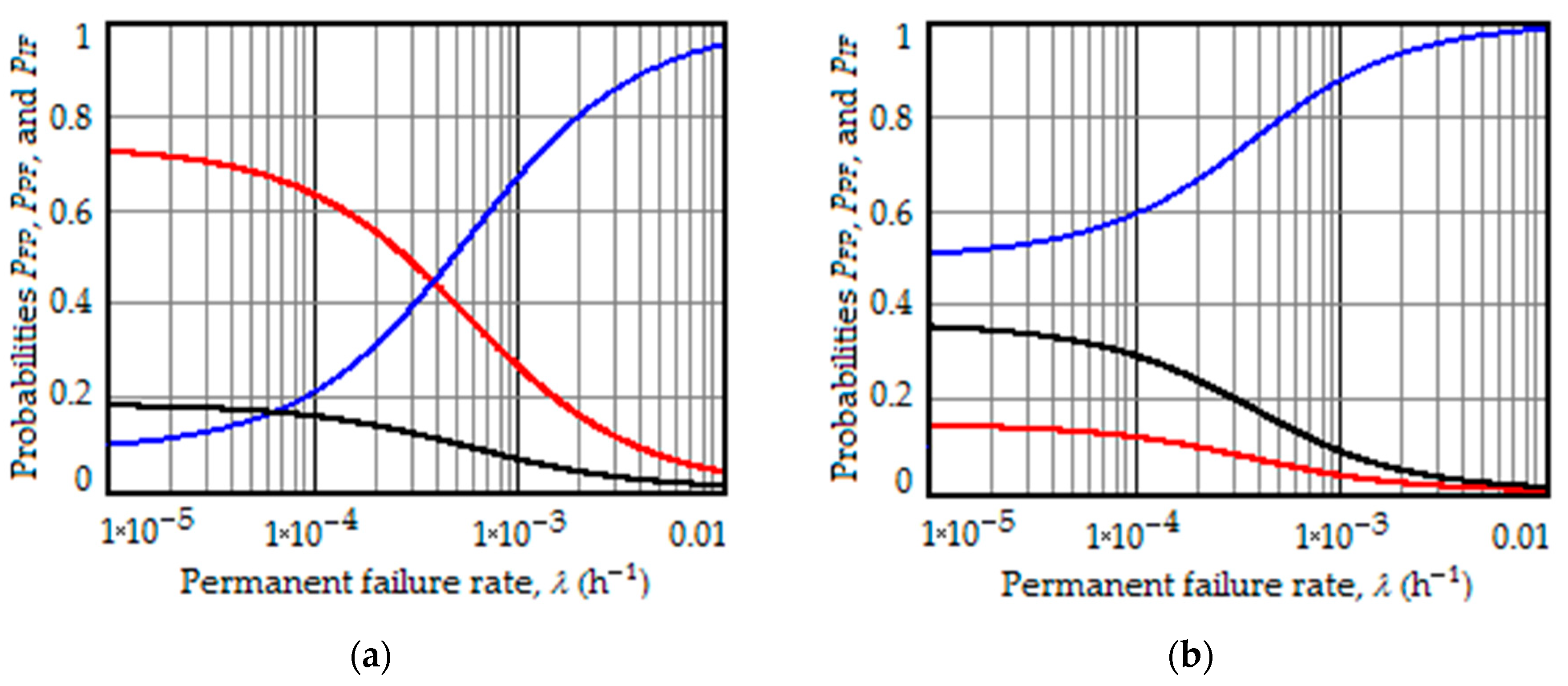
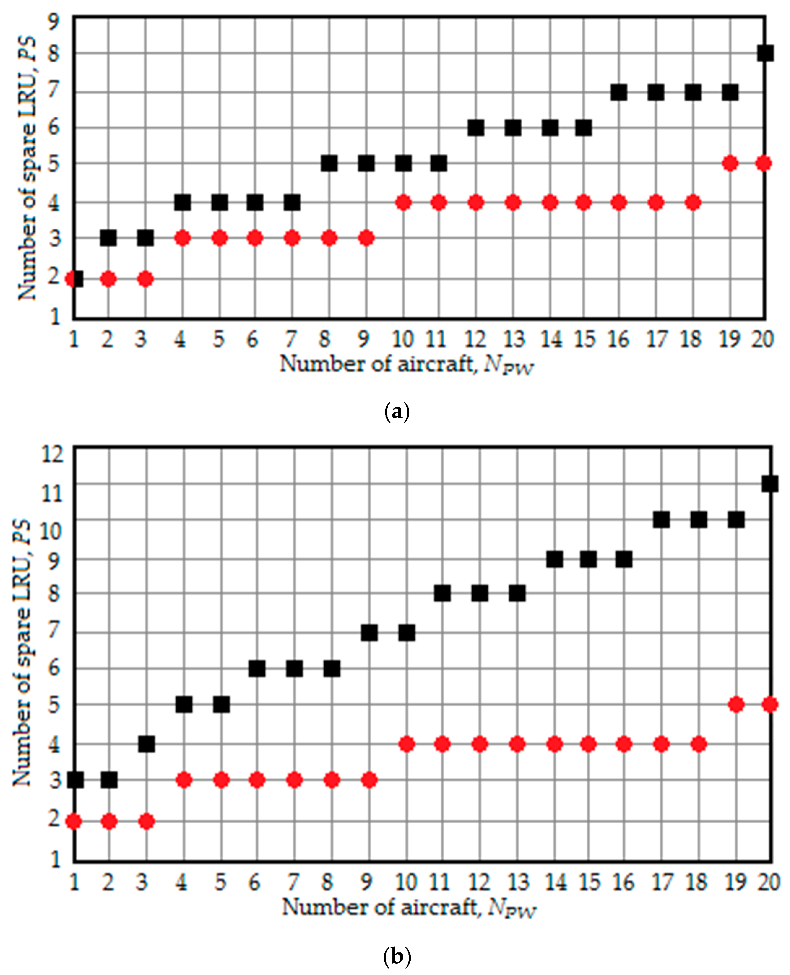
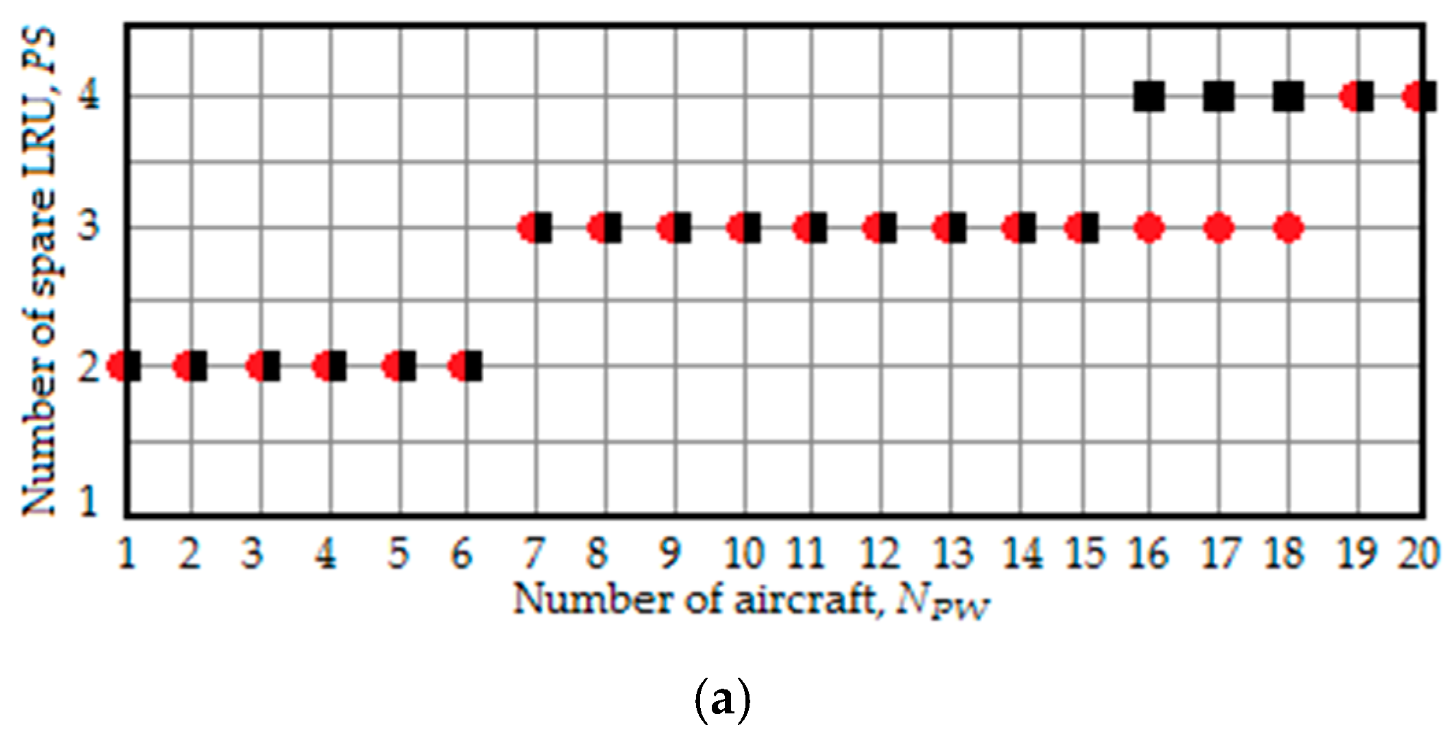
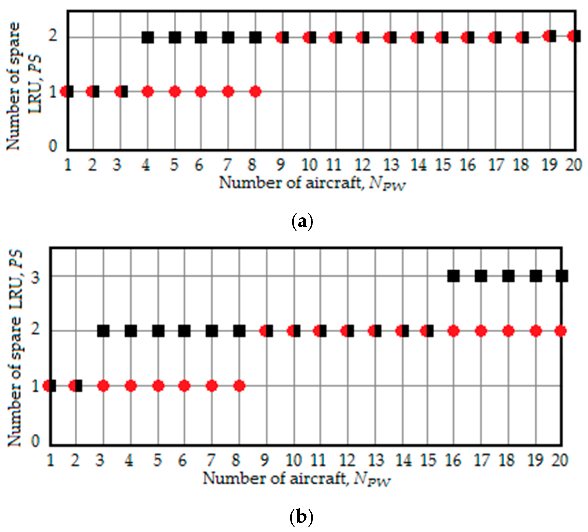
Table 1.
The calculated results for the options of warranty maintenance.
| Warranty Maintenance Opton (i) | Quantity of Planned Spare ADIRU (PS) | Quantity of Unplanned Spare ADIRU (US) | Maintenance Cost during the Warranty Period |
|---|---|---|---|
| i = 1 | 2 | 0 | $7800 |
| i = 2 | 2 | 0 | $10,400 |
Table 2.
The results of the calculations for the five post-warranty maintenance options.
| Warranty Maintenance Option (i) | MTBUR on Finite Time Horizon | Quantity of Planned Spare ADIRU (PS) | Quantity of Unplanned Spare ADIRU (US) | Maintenance Cost during the Post-Warranty Period |
|---|---|---|---|---|
| i = 1 | 21,970 h | 5 | 0 | $38,380 |
| i = 2 | 21,970 h | 4 | 0 | $31,510 |
| i = 3 | 21,970 h | 2 | 0 | $5050 |
| i = 4 | 25,570 h | 2 | 0 | $5960 |
| i = 5 | 25,570 h | 2 | 0 | $3480 |
Publisher’s Note: MDPI stays neutral with regard to jurisdictional claims in published maps and institutional affiliations. |
© 2021 by the authors. Licensee MDPI, Basel, Switzerland. This article is an open access article distributed under the terms and conditions of the Creative Commons Attribution (CC BY) license (http://creativecommons.org/licenses/by/4.0/).
Share and Cite
MDPI and ACS Style
Raza, A.; Ulansky, V. Through-Life Maintenance Cost of Digital Avionics. Appl. Sci. 2021, 11, 715. https://doi.org/10.3390/app11020715
AMA Style
Raza A, Ulansky V. Through-Life Maintenance Cost of Digital Avionics. Applied Sciences. 2021; 11(2):715. https://doi.org/10.3390/app11020715
Chicago/Turabian StyleRaza, Ahmed, and Vladimir Ulansky. 2021. "Through-Life Maintenance Cost of Digital Avionics" Applied Sciences 11, no. 2: 715. https://doi.org/10.3390/app11020715
Note that from the first issue of 2016, this journal uses article numbers instead of page numbers. See further details here.