
Empirical Approach to Defect Detection Probability by Acoustic Emission Testing
by
 ,
,
Vera Barat
1,*, 
Artem Marchenkov
1,
Valery Ivanov
2,
Vladimir Bardakov
1,3,
Sergey Elizarov
3 and
Alexander Machikhin
1,4 1
Institute of Information Technologies and Computer Science, National Research University “Moscow Power Engineering Institute”, Moscow 111250, Russia
2
Research Department, JSC RII “Spectrum”, Moscow 119048, Russia
3
Research Department, LLC “Interunis-IT”, Moscow 111024, Russia
4
Acousto-optic Spectroscopy Laboratory, Scientific and Technological Center of Unique Instrumentation, Russian Academy of Sciences, Moscow 117342, Russia
*
Author to whom correspondence should be addressed.
Appl. Sci. 2021, 11(20), 9429; https://doi.org/10.3390/app11209429
Submission received: 14 September 2021
/
Revised: 7 October 2021
/
Accepted: 8 October 2021
/
Published: 11 October 2021
(This article belongs to the Special Issue Elastic Waves and Acoustic Emission for Innovative Monitoring of Structures and Engineering Systems)
Abstract
:Estimation of probability of defect detection (POD) is one of the most important problems in acoustic emission (AE) testing. It is caused by the influence of the material microstructure parameters on the diagnostic data, variability of noises, the ambiguous assessment of the materials emissivity, and other factors, which hamper modeling the AE data, as well as the a priori determination of the diagnostic parameters necessary for calculating POD. In this study, we propose an empirical approach based on the generalization of the experimental AE data acquired under mechanical testing of samples to a priori estimation of the AE signals emitted by the defect. We have studied the samples of common industrial steels 09G2S (similar to steel ANSI A 516-55) and 45 (similar to steel 1045) with fatigue cracks grown in laboratory conditions during cyclic testing. Empirical generalization of data using probabilistic models enables estimating the conditional probability of record emissivity and amplitudes of AE signals. This approach allows to eliminate the existing methodological gap and to build a comprehensive method for assessing the probability of fatigue cracks detection by the AE testing.
1. Introduction
AE testing has become a popular and rapidly developing method of non-destructive testing (NDT) due to its unique characteristics such as high sensitivity to the presence of microcracks and the applicability to various materials. AE testing is based on the generation and analysis of elastic waves with irreversible changes in the internal structure of the material [1]. AE testing is successfully applied to testing materials with a complex structure—anisotropic magnesium alloys [2], TRIP/TWIP steels [3], and composites [4]. However, the high sensitivity and specificity of AE testing causes a number of problems that hinder its widespread use, for instance, low repeatability and low POD. There are three main reasons for the difficulties in assessing POD and interpreting the results.
First, unlike most NDT techniques, AE diagnostic signals are not a reaction to a certain probing effect. AE waves are generated by the internal sources appearing within the microstructure of the material activated during the mechanical or thermal loading [5,6]. Even when the loading pressure is determined and repeatable, the AE data is principally random. There is a strong relationship between AE signals and parameters of the material microstructure, such as the grain size, state of grain boundaries, presence and volume fraction of non-metallic inclusions, etc. [7,8,9]. The total effect of these stochastic factors explains the great variability of AE signals even for the typical testing structures and defects of similar type and size [10,11].
The second reason is the absence of a direct correlation between AE data and defect size [12]. A defect in AE testing is considered not as a discontinuity, but as an active source of elastic waves. In the case of a crack, generation of AE waves may be caused by deformation and fractures as well as by friction between existing defective surfaces, but in the case of corrosion, the most powerful AE signals may be caused by concomitant processes, such as hydrogen bubble formation or corrosion products crumbling [13,14].
The third reason is the complexity of the diagnostic data—a single defect can generate hundreds and even thousands of AE signals. It complicates formulating the defect detection criteria, unlike other NDT methods where the defect may be detected from a single signal when its amplitude exceeds a certain threshold.
Due to the presence of residual stresses, generation of AE is also possible for defect-free structures, which contributes to the probability of making false detection of a defect (type I error). In the presence of a defect, signals corresponding to its growth must be identified against the background of external acoustic noise, which increases the probability of defect omission (type II error). One of the first approaches to assessing defect detection probability is described in [15,16]. This approach represents a universal method for estimating POD in the case of fatigue destruction, but their implementation requires setting more than 20 quantitative a priori unknown parameters. An empirical method for assessing POD in composite materials is based on the distribution of AE hit amplitudes using a finite element model of the acoustic waveguide [17]. Various aspects are analyzed in [18,19], with respect to POD at various stages of defect development and the likelihood of correctly assessing the defect hazard class. In [20,21], a method for calculating POD in industrial objects made of ductile low-carbon steel is proposed. Based on the experimental data, the authors justify the need to scale the amplitude distribution by the crack step value, while POD turns out to be proportional to the crack size. The reliability of defect detection by the AE method in composite materials is also considered in [22], where the author compares the distribution of the defect’s dimensions with the distribution of AE hit amplitudes and estimate the probability of making type I and II errors by comparing the discrimination threshold value with the quantile of the amplitude distribution.
The problem of assessing POD in AE testing cannot be solved in general due to uncertain stress–strain conditions and a strong influence of the material microstructure. Partial decisions for POD estimation are possible but do not have a practical meaning. This study represents an attempt to make a reasonable generalization in assessing POD for AE testing. The proposed method allows estimating POD for the case of periodical AE inspection and for the steels of the pearlitic structural class.
Periodic AE testing procedure is carried out for the decommissioned structures and, in contrast to structural health monitoring, assumes a certain regulated loading procedure, which represents a stepped pressure loading of the structure. With such organization of the testing procedure, the stress–strain state of the structure is not completely uncertain. Restrictions on the structural class of the investigated steels allow making more definite generalizations regarding the parameters of AE sources.
In [12], it was proposed to predict the number of AE hits emitted by an object with crack during the loading procedure using the Palmer–Heald model, which represents the relationship of the number of AE hits vs. the applied load up to a multiplicative parameter D, which is a constant of the inspected material. Based on the analysis of experimental data for different steels of the same structural class, it was shown that this parameter can be interpreted as a random variable with a normal distribution with constant parameters (mean value and variance) for certain steel grades. Refinement of the parameters of the Palmer–Heald model enables predicting the crack type from AE source emissivity with a certain probability.
Though such a model does not clarify the nature and hazard class of AE source, its application makes it possible to estimate statistically the number of AE hits emitted by AE source, and together with AE hits amplitude distribution allows predicting detectability and assessing POD.
This paper represents an approach to assessing the probability of fatigue crack detection by AE testing. For this aim, we offer an a priori model of the AE testing procedure, which includes a model of the AE source, allowing to predict the emissivity and the amplitudes of AE signals, as well as a model of the waveguide, allowing to predict the signals’ waveform. The procedure for AE data processing is also simulated.
A kind of concentration criterion is considered as a detection criterion, in which a defect is detected if the location cluster reaches a certain density. The main efforts of the authors are aimed at determining the probability of fulfilling the defect detection criterion for various AE test parameters, such as the distance between the sensors, the maximum load value, the steel grade, etc.
The following assumptions are made in the frame of this study:
- -
- fatigue cracks originate and propagate under cyclic operating load and are detected during AE testing under step loading by tension, as recommended by the ASTM standard [23];
- -
- during the AE data registration, the method of threshold detection is used, while the threshold value is refined based on the calculation of the probability of defect detection;
- -
- as a method of location, linear location is considered, while the density of the cluster is determined as the number of AE events located at an interval of 0.05L, where L is the distance between the AE sensors.
2. Materials and Methods
We have studied the notched samples made from hot-rolled sheets with a thickness of 3–5 mm made of industrial steels 09G2S (similar to steel A 516-55) and 45 (similar to steel 1045) with a ferrite–pearlite structure and nominal chemical composition shown in Table 1 [12].
The samples were tested under static tension using a loading schedule described in [23]. Flat samples with an edge notch were made according to ASTM E1930/E1930M-17. In total, 50 samples were made of 09G2S steel and 10 samples of steel 45. Fatigue cracks were grown in all samples by cyclic tensile loading with a maximum cycle stress of σmax ≈ 0.6·σy (σy is the yield strength). The loading stops when fatigue crack developing in the lateral notch area reaches a certain length. Nominal crack lengths vary from 3 to 15 mm. Thus, the total length of the notch and crack is 15 to 28 mm depending on the sample.
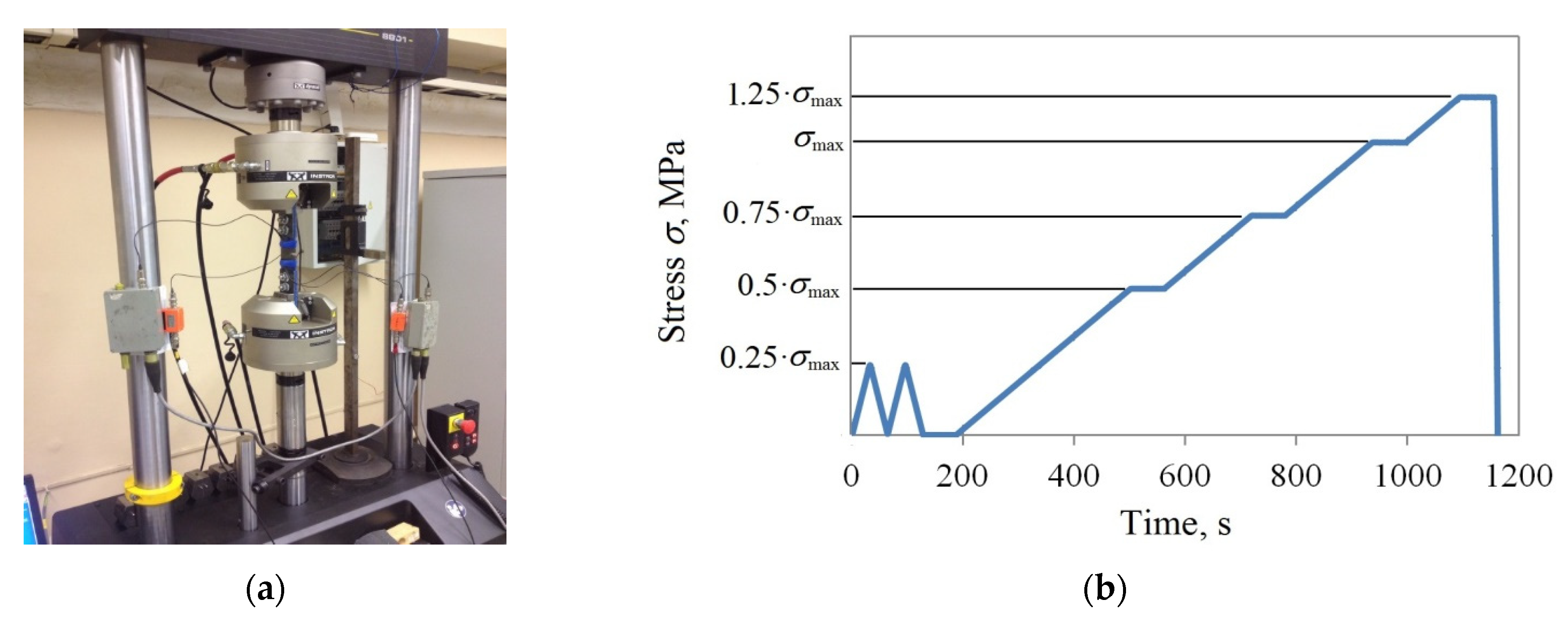
At the next stage, testing of the samples with fatigue cracks was carried out by Instron 8801 testing machine (Figure 1a). AE signals were recorded during the tests using A-Line 32D industrial system. The measuring path consisted of resonant sensors GT200 (LLC “Global test”) which have resonance frequency 180 kHz and preamplifiers of the electrical signal PAEF-014. The total noise of the equipment is 26 dB in reference to 1 µV at preamplifier input. The threshold for acoustic signals discrimination was set to 40 dB.
The loading diagram is shown in Figure 1b. Two triangular cycles at the initial stage are necessary to equalize the internal mechanical stresses that occurred during the production and placing of the samples. The main loading cycle consists of four stages: first, the load gradually increases from 0 to 0.5 σmax, second—from 0.5 σmax to 0.75 σmax, third—from 0.75 σmax to σmax. The fourth stage is carried out with a stress exceeding σmax by 25%. A more detailed description of the experiment is given in [12].
3. POD Estimation
Simplified probability estimation algorithms are shown in Figure 2. To assess the probability of making a type I error associated with a false defect detection, long-time realizations of noise should be obtained. For each realization, a processing procedure is carried out to verify the defect detection criterion. The correct completion of the check procedure is the deviation of the criterion fulfillment condition, otherwise, a type-I error occurs. The probability of making type-I error α is defined as the number of erroneous decisions k to the total sample size N, i.e., .
The probability of making a type-II error is estimated similarly based on a priori models of the AE data set. The stochasticity of the AE source parameters provides a difference in the AE parameters of the sample. The probability of making a type-II error β is defined as the number of cases when the detection criterion is not fulfilled m to the total sample size N, i.e., .
3.1. Empirical AE Signals Modeling
To assess the POD, we have developed an algorithm for a priori estimation of AE data sampling parameters. The main stages of this algorithm are the probabilistic model of the AE source and the deterministic model of the waveguide.
During industrial AE testing, when the distance between sensors and source can reach several meters, AE source parameters do not significantly affect the AE signal waveform. Therefore, we may assume that the AE source emits short impulses (δ-impulses) with duration less than the sampling period. Thus, the AE source emits N∑ signals with amplitudes Ak, k ϵ [1, N∑]. N∑ and Ak may be considered as random variables. A detailed description of the AE source is presented in paragraph 3.1.1.
Signal waveform is mainly determined by the dispersive propagation along the waveguide. Thus, to calculate the AE signal waveform, a waveguide model is necessary. In this study, we use an analytical model of the waveguide, which allows calculating the dispersive AE signals propagation. The waveguide model is described in paragraph 3.1.2.
The flowchart of the simulation algorithm is shown in Figure 3. To make the model more realistic, noise may be added to the AE signal.
As a result of the modeling, we obtain the AE data set which is regarded as a separate AE signal. The number of signals and their amplitudes Ak are determined by AE source and the waveform f(t) is the function of the waveguide.
3.1.1. AE Source Modeling
The defect is the AE source, which responds to the loading effect and emits signals with a nanosecond duration and can be considered as δ-functions. The number of emitted signals N∑ and the amplitudes of the AE signals Ak depend not only on the defect size, but also on the loading parameters and, to a large extent, on the parameters of the material microstructure. Preliminary studies have shown that the parameters N∑ and Ak can be considered as random variables that do not directly correlate with the defect size. In [12], it was established that the parameters N∑ and Ak correspond to certain laws of probability distribution and can be estimated using probabilistic models.
The number of signals emitted by a defect during growth per unit length is a parameter of the material emissivity and can be estimated using the multiplicative parameter of the Palmer–Heald model as
where σ is the actual stress, σy is yield stress, Da is coefficient depending on the characteristics of the material [24]. The parameter Da is random and corresponds to the normal distribution N(μ,σ2) and the quantitative values of μ and σ2 for 09G2S and 45 steels are given in [12]. According to the well-known law of Da probability distribution, based on the Palmer–Heald model, it is possible to estimate the probability that a certain number of AE signals will be recorded when the object with fatigue crack is loaded. For this, the distribution of Da is scaled by the coefficient with respect to the value σmax.
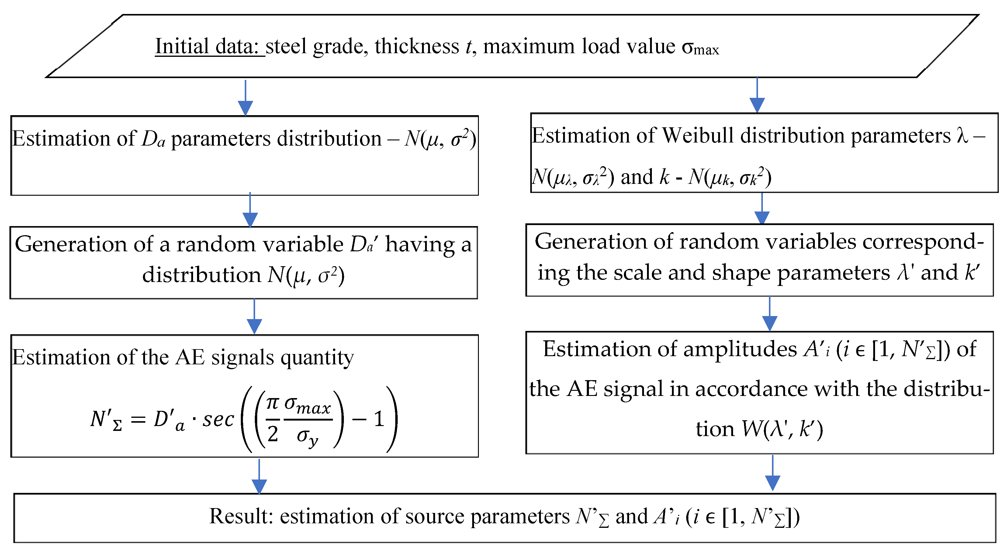
In [25], it was shown that the distribution of AE signal amplitudes corresponds to the Weibull law W(λ,k). The parameters of scale λ and shape k are random values corresponding to the normal distribution law for each of the inspected materials. Considering the results of the preliminary study, a hierarchical two-level algorithm is proposed for modeling the AE source (Figure 4), in which the distribution parameters for λ, k and Da are estimated first, and then the parameters of the AE source are determined, characterizing its emissivity and amplitude values of radiated AE signals.
3.1.2. Modeling the Parameters of the Acoustic Waveguide
The signal waveform f(t) is determined by the patterns of its propagation along the acoustic path. Various analytical, semi-analytical or numerical models may be used to simulate the signal shape. In this study, to calculate the acoustic waveguide, an analytical algorithm for calculating the normal waves propagation [26] was used, based on the modal analysis [27] and analytical calculation of the frequency-dependent attenuation coefficient [28]. The modeling of the acoustic path (Figure 5) is described in detail in [26].
3.2. Defect Detection Probability Calculation
AE signal parameters modeling described in the previous section makes it possible to implement an algorithm for calculating POD as a detailed numerical experiment, including modeling AE signals about variations in the values of a priori unknown defect parameters.
The initial data are the steel grade, wall thickness, parameters of liquid media, maximum value of the applied mechanical load, frequency range, and characteristics of AE sensor. Based on specified initial parameters, considering the different locations of the defect, the calculation of realistic models of AE signals has been carried out. The coordinate of the defect varies from 0 to L with a step Δx, where L is the distance between the sensors that form the location sensor array. Models are calculated for two AE sensors that form the linear location. Each of the models is formed for the same source parameters N’∑ and A’i (i ϵ [1, N’∑]) with the distance from the defect x and L-x, respectively.
Since the formation of a location cluster of a certain density is considered as a criterion for defect detection, a location procedure is carried out to check the detection condition, followed by an assessment of the formed location cluster density.
In accordance with regulatory documentation, the location error is about 5% of the distance between the sensors L. Therefore, the density of the location cluster is determined over the interval length as , where Nclust is the number of indications in the location interval. The flowchart of this algorithm is shown in Figure 6.
A defect is detected if the location cluster has reached the critical density . Otherwise, a type-II error occurs. Since the simulation is based on the probabilistic model of the AE source, to obtain a reliable POD, it makes sense to repeat the calculation procedure ~104–106 times. POD at a certain location is determined as the fraction of the total number of repetitions N, at which the detection condition is satisfied. For the case of an arbitrary and a priori unknown location of the defect, POD is determined as
3.3. Calculating Probability of Making Type-I Error
One of the significant disadvantages of AE testing is the presence of external noise associated with technological processes of the testing structure or with the loading process. The most common sources of noise include friction, fluid leakage, bubbling and cavitation, and various types of electrical and electromagnetic noise. This section provides a methodology for calculating the type-I error probability associated with false defect detection. To calculate the probability of false detection, it is necessary to calculate the probability of the location cluster formation in the absence of a defect. We assume that the noise parameters are constant throughout the entire testing procedure. The initial data for calculation are the probability distribution density of the noise process, the value of the amplitude discrimination threshold thr, location parameters, distance between the AE sensors L and the sound velocity c. The probability p is estimated from the condition that the samples of the time realization of noise(t) exceed a certain threshold value thr:
For the AE event to be located and displayed on the location diagram as an indication, the difference Δt in the recording times of signals must satisfy the inequality , where c is the velocity of AE waves propagation. The probability of locating the noise signal ploc can be calculated as the probability that the difference in the arrival times of signal recorded by the sensor array channels will be less than Δt. For this, Poisson’s formula is appropriate. It allows calculating the probability of a false location as:
where fd is the sampling rate of the AE signal.
For uncorrelated noise, the probability of a false indication ploc can be calculated as . For correlated noise, it is . According to the selected criterion for defect detection, the probability of making a type-I error is estimated as the probability of the appearance of Nclust indications in the interval ΔL. To estimate the probability of such an event, it is necessary to set the total measurement time T, since the type-I error increases with the increase of the number of recorded noise samples. The probability of an error α can be estimated using the Poisson formula as the probability of occurrence of Nclust events with the probability ploc when the number of trials is T/Δt:
4. Results and Discussion
4.1. AE Signal Simulation Results
A priori determination of AE source parameters is one of the main results of this study. According to the proposed model, the emissivity of fatigue crack may be estimated using the multiplicative coefficient Da of the Palmer–Heald model (1). For fractures at the stage of stable growth, it corresponds to the normal distribution law.
Table 2 shows mean values and standard deviations of parameter Da, obtained on the basis of empirical data for the studied steel grades with respect to the wall thickness of the investigated object. According to the distribution of Da, it is possible to estimate the probability that a certain number of AE signals will be recorded when an object with fatigue crack is loaded.
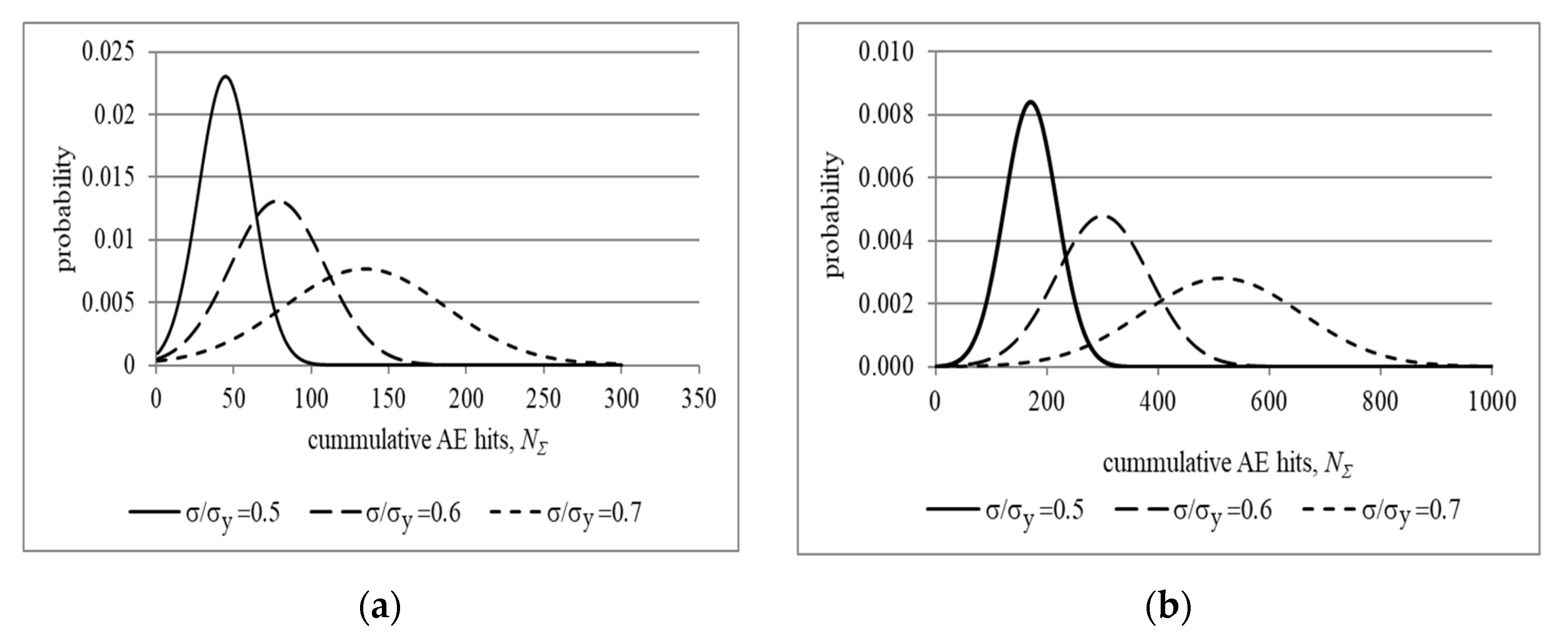
Figure 7 shows the density distribution of the AE hits quantity NΣ for steels 09G2S and 45 at different maximum values of mechanical stress in the loading cycle. A high emissivity of steel 45 is noted as compared to steel 09G2S; in addition, an increase in the maximum mechanical stress σmax from 0.5σy to 0.7σy leads to an increase in NΣ by on average three times.
When analyzing the amplitude distribution, we have found that for fatigue cracks in 09G2S and 45 steels at the stage of stable growth, amplitude distribution follows the Weibull distribution law. Moreover, the distribution of the parameter λ corresponds to the normal distribution law with parameters μ = 5.5 and σ = 1.13 for steel 09G2S, μ = 7.76 and σ = 0.69—for steel 45. The parameter k is characterized by a small scatter and for both steels can be represented using the normal distribution with the parameters μ = 1.14 and σ = 0.095.
Figure 8a shows the Weibull distribution functions for the mean value of the scale parameter within the confidence interval of the parameter k with a confidence level of 0.95. Figure 8b shows the Weibull distribution functions for the mean value of the parameter k within the confidence interval (3.25, 7.77) of the parameter λ with the same confidence value of 0.95. These dependencies show that the scatter of the shape parameter has a significantly smaller effect on the distribution type than the spread of the scale parameter. The obtained values of AE emissivity and parameters of the impulse amplitude distribution correspond to the data presented in [29,30,31].
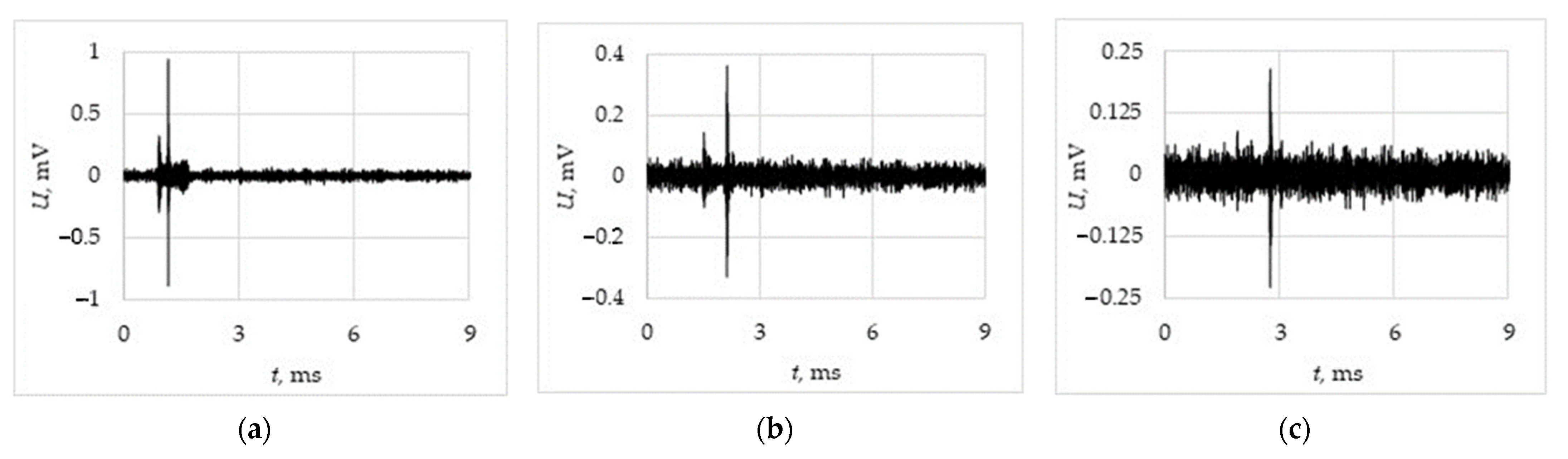
Examples of AE signal waveforms obtained as a result of modeling are shown in Figure 9 and Figure 10. Figure 9a–c shows the signals calculated in accordance with the method described in paragraph 3.2.1, for the distances between the AE source and AE sensor of 2, 5, and 7 m, respectively. Figure 10 shows more realistic data: modeled signals are shown against the background of noise caused by the pump during hydraulic loading. The correctness of AE signal simulation and their correspondence to the experimental data are demonstrated in [26].
The AE waveforms shown in Figure 9 and Figure 10 are the components of the signals s1 (formula 3) and s2 (formula 4), which are used to determine the location of the AE source. Figure 10 shows an example of calculating the location of a fatigue crack in steel 45 with parameters based on the distributions shown in 7b and 8b (N∑ = 250, λ = 7.76, k = 1.13). The distance between the AE sensors L was set equal to 7 m, the source coordinate x = 2 m. Figure 11a–c corresponds to different values of the discrimination threshold—30, 35, and 40 dB, respectively. The best location result corresponds to a lower discrimination threshold; with an increase in the threshold, the location error is associated with an incorrect determination of the arrival time of the AE signals and a small number of localized events with missed AE signals, the amplitude of which was less than the discrimination threshold.
4.2. Results of Estimating Type II Error Probability
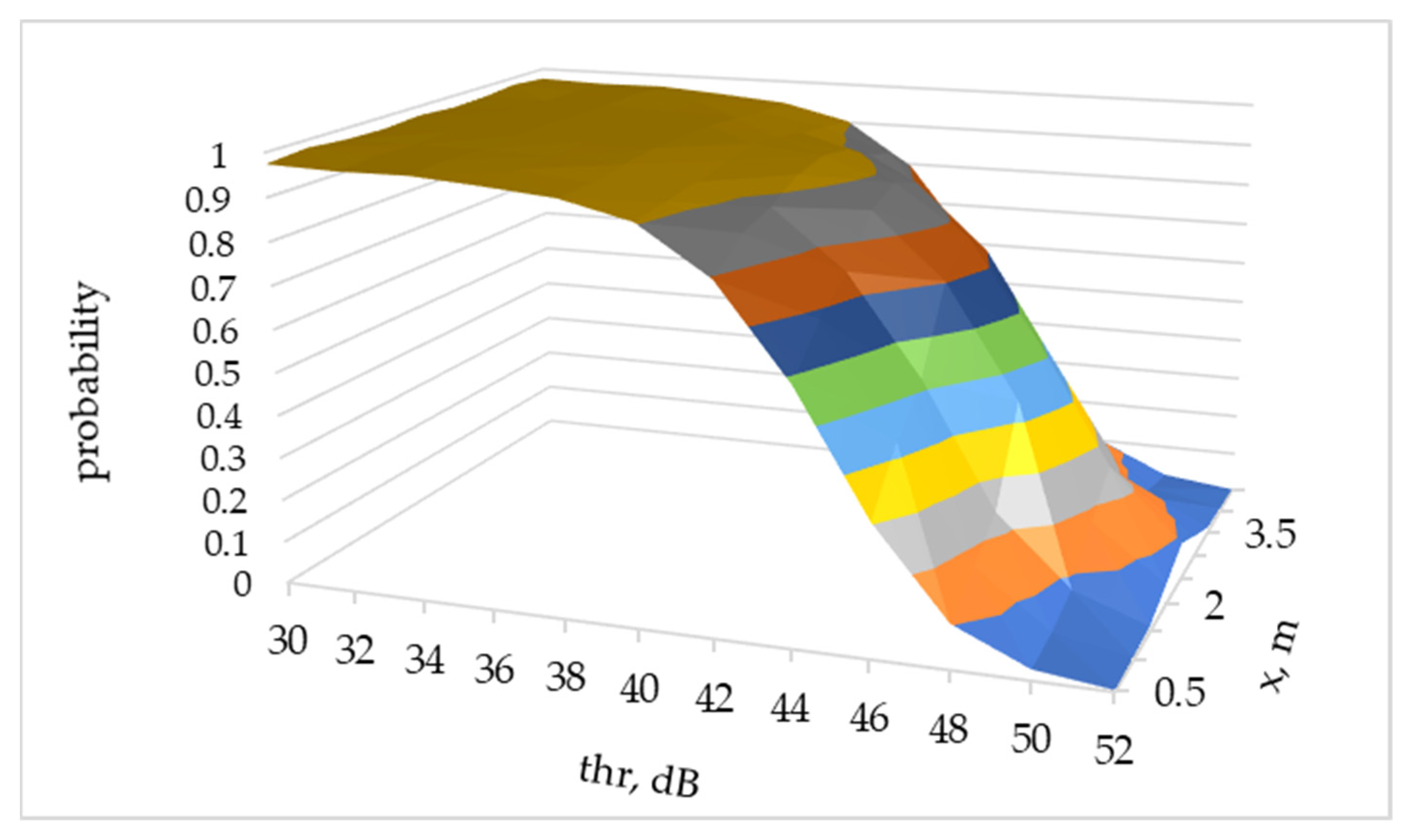
Figure 12 shows the POD values versus detection threshold and various values of the defect coordinate x (x = 1..L) calculated for Nclust = 5 and the distance between the sensors L = 5 m. The POD depends significantly on the threshold value. For threshold values of 40 dB, 45 dB, and more than 48 dB the POD value is 95%, 83%, and less than 50% respectively, for the case when a defect is placed in the middle between the sensors (x = 2.5 m).
The dependence of the POD on the coordinate x is less significant. The highest POD is reached when the defect is placed in the middle between the sensors. When the defect is displaced from the central part, the probability decreases. For example, at a threshold of 40 dB and 45 dB the POD decreases by 5% and 35%, respectively, when the defect coordinate changes from x = 2.5 m to x = 0.5 m
Figure 13 shows the dependence of POD on the amplitude discrimination threshold for L = 5 m at different values of Nclust, which determines the number of located events. The probability of a fatigue crack detection decreases with an increase in the threshold thr, and the rate of decrease initially becomes higher with the increase of Nclust.
The probability of AE signal detection for steel 45 is significantly higher than for steel 09G2S. The maximum value of the discrimination threshold, which ensures reliable defect detection, is 10 dB higher for steel 45 than for steel 09G2S. Therefore, fatigue cracks in steel 45 can be detected at a higher noise level. For example, with a detection threshold of 40 dB and a distance between the sensors L = 5 m, the probability of detecting a fatigue crack in steel 45 is 8% higher than in steel 09G2S, and at a threshold of 45 dB, typical for noisy objects, the probability of detection for steel 45 is higher by 32%.
Calculating the probability of fatigue crack detection at different distances between the AE sensors was carried out according to the algorithm described in Section 3.2. The probability of fatigue crack detection versus testing zone length, given by a distance between the AE sensors is shown in Figure 14. The calculation was carried out for a single-layer waveguide, not in contact with a liquid.
The probability of detecting a fatigue crack in steel 45 is significantly higher at any distance between the AE sensors. For example, with a minimum threshold value of 30 dB, the detection probability of 0.95 corresponds to the L = 8 m for steel 09G2S and L = 16 m for steel 45.
Comparing the probabilities of detecting fatigue cracks for different distances between the sensors, it can be noted that at L = 10 m the probability of detecting cracks in 09G2S and 45 steel is approximately the same, and at L = 15 m the probability of detecting a crack in 45 steel is approximately 20% higher. However, a further comparison is impractical, since at L > 20 m the probability of detecting a crack in 09G2S steel is less than 50%.
4.3. Results of Estimating the Type-I Error Probability
In this study, we considered signals of two types as noise: stationary noise generated by the compressor of the loading device and unsteady impulse noise caused by turbulent fluid flow inside the object under test. Figure 15a,b shows the temporal realizations of this noise. Figure 15c,d illustrates the probability distribution density.
The distribution of stationary noise is close to normal, while the distribution of non-stationary noise is different from the normal due to a heavy tail formed with an outlier’s samples. With a standard time of AE testing of about 1 h and an average sampling frequency of ~5 MHz, about samples are analyzed during the testing time.
Figure 16 shows the POD calculation results obtained using the method described in paragraph 3.3 for stationary uncorrelated and stationary correlated noise at L = 5 m. For uncorrelated noise, the probability of type-I error turned out to be significantly lower than for correlated noise. This can be explained by the fact that the statistical independence of uncorrelated data measured by different AE channels reduces the probability of a false location. A sharp increase in the probability of false detection for uncorrelated noise is observed at a threshold of about 6 std, for correlated noise—at 4 std; therefore, at the same noise level, the detection threshold for uncorrelated noise can be 1.5 times lower than for correlated noise. An increase in the required number of indications in a location cluster from 5 to 20 allows reducing the value of the data registration threshold by 0.7 dB, which is an insignificant value in terms of a better likelihood of detection.
Figure 17 shows the result of a type-I error probability calculation for the case of non-stationary noise. The impulse nature of the noise (Figure 15b) requires the detection threshold to be significantly higher than for stationary processes.
An acceptable value of the probability of a type-I error is achieved at a threshold of the order of 10–15 std. At the same time, an increase in the Nclust parameter from 5 to 20 makes it possible to reduce the threshold by at least 4 dB at the same error level.
4.4. Selection of the AE Testing Parameters Based on Minimizing the Total Error Probability
The threshold value and the value of the parameter Nclust are the setting constants during the probability calculation. An increase of Nclust and thr leads to a decrease of a type-I error probability and an increase in the probability of a type-II error. A decrease in these parameters, on the contrary, decreases the probability of a type-II error but increases the probability of a type-I error. The correct choice of Nclust and thr allows finding a compromise—to achieve a minimum of the total error probability, which can be estimated from the probabilities of type-I α and type-II β errors as:
where π0, π1 are a priori probabilities of the events associated with the occurrence of type-I and -II errors. Minimization of the total error probability is one of the criteria for optimal detection that can be used as a criterion for optimal defect detection [32].
To determine the optimal detection parameters, the dependences obtained in Section 4.3 were scaled in accordance with the specified value of the noise standard deviation. Figure 18a–c shows the probability of type-I and -II errors at different thr for the correlated noise with standard deviation std = 25, 27.5, and 30 dB, respectively. Figure 18d–f illustrates the dependences of the total error probability on the discrimination threshold for various noise levels.
As follows from Figure 18 d–f, the minimum total error probability is achieved at the minimum value of the parameter Nclust = 5 at a threshold approximately equal to 6 std. At a noise std = 25 dB, the minimum possible value of the total error probability is 5%, at a std = 27.5 dB—14% and at a std = 30 dB about 31%. The influence of the parameter Nclust is greater for higher noise levels. At std = 25 dB, the total error probability corresponding to Nclust = 5 is 5% greater than at Nclust = 20, and at std = 30 dB, increasing Nclust from 5 to 20 leads to an increase in the minimum value of the total error probability by 18%
Figure 19 shows the minimum total probability depending on the threshold for various Nclust for stationary uncorrelated, stationary correlated, and non-stationary frictional noise. For all types of noise, the minimum values of the total error probability are reached at Nclust = 5. The value of the total error probability significantly depends on the noise type. A total error probability of less than 0.1 is achieved for uncorrelated stationary noise with s <30 dB, for correlated stationary noise—with s <26 dB, and for non-stationary frictional noise—with s <18 dB.
5. Conclusions
In this study, we have proposed a new approach to assessing the probability of fatigue cracks detection in structural steels during AE testing, based on an a priori estimation of AE signals emitted during crack growth with respect to the parameters of the acoustic waveguide and data registration, such as amplitude discrimination threshold and spatial filtration. We have implemented an empirical approach, i.e., the parameters of the AE source have been determined experimentally. However, the probabilistic assessment of the crack emissivity and the values of the AE signals amplitudes enables generalizing the results obtained for a class of steels with a ferrite–pearlite structure.
The parameters of the AE source—the number of emitted signals during the growth of the crack (emissivity) and the amplitudes of the AE signals are estimated as random parameters (Figure 6). The parameters of the acoustic path, on the contrary, are considered deterministic using analytical modeling of dispersive propagation and frequency-dependent attenuation of AE waves. The integration of mathematical models of various types has been carried out (Figure 8), which allows calculating AE signal which corresponds to different values of the source parameters and reflecting the variability of the AE parameters observed during the testing procedure in an industrial environment. Due to a large number of random parameters, the calculation of the AE parameters using the empirical model is carried out about 10,000 times, until the estimated value of the probability stabilizes, i.e., the estimated value does not change by more than 0.05% within 100 iterations.
The proposed approach is based on the statistical model of the source; therefore, it is more formal than the approach based on Paris law and the AE source theory [33] represented by Pollock [15]. In addition to the statistical basis, the present method utilizes a physical Palmer–Heald model, therefore being more reliable and specific than methods based on artificial neural networks [34] and deep learning technology [35].
The proposed method is relatively complex since it represents a common concept, which allows considering many factors influencing the AE test result. However, the method in its current state has several simplifications that should be revised in a more detailed examination or for more specific test conditions:
- -
- when calculating the probability of defect detection, it is assumed that the AE channels have the same sensitivity. However, in practice, the sensitivity may differ due to problems associated with the quality of the acoustic contact between the transducer and the testing object; the information about testing structure—sensor coupling could be obtained during the calibration of the AE equipment,
- -
- during data analysis, the authors rely on the amplitude distribution and the emissivity parameter, however, the use of precise broadband sensors allows considering information in the frequency domain, which, in turn, allows us to change the defect detection criterion, making it more reliable for solving specific problems.
- -
- probability calculation is carried out only for a given detection criterion during standard data processing, including only threshold discrimination and standard location procedure.
The proposed technique opens wide possibilities for POD assessment under various testing conditions. It is possible to consider the distance between the AE sensors, the magnitude of the maximum applied load, AE sensor parameters, noise characteristics, etc.
For example, it was shown that for structures made of steel 09G2S, AE testing may provide 95% POD at 10 m distance between sensors and 30 dB detection threshold as well as at 5 m distance and 40 dB threshold. For steel 45 with higher AE emissivity, the distance between the sensors may be greater: 18 m at 30 dB threshold and 12 m at 40 dB threshold.
The optimum threshold value could be estimated during the total error probability minimization.
The modular structure of the proposed algorithm allows independent refinement of AE source and waveguide models without changing the general calculation concept. The proposed methods may be used to estimate the probability of fatigue crack detection during industrial AE testing of extended objects undergoing cyclic loads: pipelines, tanks, pressure vessels, etc.
Author Contributions
Conceptualization, V.B. (Vera Barat) and V.I.; methodology, V.B. (Vera Barat); experiment, A.M. (Artem Marchenkov); validation, V.B. (Vladimir Bardakov), S.E.; formal analysis, A.M. (Alexander Machikhin); investigation, V.B. (Vera Barat); data curation, V.B. (Vera Barat) and A.M. (Artem Marchenkov); writing—original draft preparation, V.B. (Vladimir Bardakov); writing—review and editing, V.B. (Vera Barat) and A.M. (Alexander Machikhin); visualization, V.B. (Vladimir Bardakov); supervision, S.E.; project administration, A.M. (Alexander Machikhin); funding acquisition, A.M. (Alexander Machikhin) and V.B. (Vera Barat) All authors have read and agreed to the published version of the manuscript.
Funding
The reported study was funded by Russian Foundation for Basic Research, Sirius University of Science and Technology, JSC Russian Railways and Educational Fund “Talent and success”, project 20-38-51019.
Institutional Review Board Statement
Not applicable.
Informed Consent Statement
Not applicable.
Data Availability Statement
The data presented in this study are available on request from the corresponding author.
Acknowledgments
The authors are very grateful to Kanji Ono for substantial discussion and valuable remarks.
Conflicts of Interest
The authors declare no conflict of interest.
References
- Miller, R.K. (Ed.) Acoustic emission. In Nondestructive Testing Handbook, 3rd ed.; American Society for Nondestructive Testing: Columbus, OH, USA, 2005; Volume 6, 446p. [Google Scholar]
- Shiraiwa, T.; Tamura, K.; Enoki, M. Analysis of kinking and twinning behavior in extruded Mg–Y–Zn alloys by acoustic emission method with supervised machine learning technique. Mater. Sci. Eng. 2019, A768, 138473. [Google Scholar] [CrossRef]
- Linderov, M.; Segel, C.; Weidner, A.; Biermann, H.; Vinogradov, A. Deformation mechanisms in austenitic TRIP/TWIP steels at room and elevated temperature investigated by acoustic emission and scanning electron microscopy. Mater. Sci. Eng. A 2014, 597, 183–193. [Google Scholar] [CrossRef]
- Al-Jumaili, S.K.; Eaton, M.J.; Holford, K.M.; Pearson, M.R.; Crivelli, D.; Pullin, R. Characterisation of fatigue damage in composites using an Acoustic Emission Parameter Correction Technique. Compos. Part B Eng. 2018, 151, 237–244. [Google Scholar] [CrossRef] [Green Version]
- Behnia, B.; Buttlar, W.; Reis, H. Evaluation of Low-Temperature Cracking Performance of Asphalt Pavements Using Acoustic Emission: A Review. Appl. Sci. 2018, 8, 306. [Google Scholar] [CrossRef] [Green Version]
- Kogbara, R.; Iyengar, S.R.; Grasley, Z.C.; Rahman, S.; Masad, E.A.; Zollinger, D.G. Correlation between thermal deformation and microcracking in concrete during cryogenic cooling. NDT E Int. 2016, 77, 1–10. [Google Scholar] [CrossRef]
- Richeton, T.; Weiss, J.; Louchet, F. Dislocation avalanches: Role of temperature, grain size and strain hardening. Acta Mater. 2005, 53, 4463–4471. [Google Scholar] [CrossRef]
- Vinogradov, A.; Lazarev, A.; Linderov, M.; Weidner, A.; Biermann, H. Kinetics of deformation processes in high-alloyed cast transformation-induced plasticity/twinning-induced plasticity steels determined by acoustic emission and scanning electron microscopy: Influence of austenite stability on deformation mechanisms. Acta Mater. 2013, 61, 2434–2449. [Google Scholar] [CrossRef]
- Ono, K. Current understanding of mechanisms of acoustic emission. J. Strain Anal. Eng. Des. 2005, 40, 1–15. [Google Scholar] [CrossRef]
- Zárate, B.A.; Caicedo, J.M.; Yu, J.; Ziehl, P. Probabilistic Prognosis of Fatigue Crack Growth Using Acoustic Emission Data. J. Eng. Mech. 2012, 138, 1101–1111. [Google Scholar] [CrossRef]
- Agletdinov, E.; Pomponi, E.; Merson, D.; Vinogradov, A. A novel Bayesian approach to acoustic emission data analysis. Ultrasonics 2016, 72, 89–94. [Google Scholar] [CrossRef]
- Barat, V.; Marchenkov, A.; Elizarov, S. Estimation of Fatigue Crack AE Emissivity Based on the Palmer–Heald Model. Appl. Sci. 2019, 9, 4851. [Google Scholar] [CrossRef] [Green Version]
- Andruschak, N.; Saletes, I.; Filleter, T.; Sinclair, A. An NDT guided wave technique for the identification of corrosion defects at support locations. NDT E Int. 2015, 75, 72–79. [Google Scholar] [CrossRef]
- Kietov, V.; Mandel, M.; Krüger, L. Combination of Electrochemical Noise and Acoustic Emission for Analysis of the Pitting Corrosion Behavior of an Austenitic Stainless Cast Steel. Adv. Eng. Mater. 2019, 21, 1800682. [Google Scholar] [CrossRef]
- Pollock, A. Probability of detection for acoustic emission. J. Acoust. Emiss. 2007, 25, 167–172. [Google Scholar]
- Pollock, A.A. A pod model for acoustic emission—Discussion and status. AIP Conf. Proc. 2010, 1211, 1927. [Google Scholar] [CrossRef]
- Sause, M.G.R.; Linscheid, F.F.; Wiehler, M. An Experimentally Accessible Probability of Detection Model for Acoustic Emission Measurements. J. Nondestruct. Eval. 2018, 37, 17. [Google Scholar] [CrossRef]
- Ivanov, V.I.; Musatov, V.V.; Sazonov, A.A. Accident risk analysis using non-destructive testing and technical diagnostics methods. Ind. Saf. Expertise Diagn. Hazard. Prod. Facil. 2016, 1, 37–48. [Google Scholar]
- Builo, S.I.; Chebakov, M.I. Probalistic-Information Approach to Assessing the Reliability of the Results of the Acoustic-Emission Method of Testing and Diagnostics. Russ. J. Nondestruct. Test. 2021, 57, 375–382. [Google Scholar] [CrossRef]
- Builo, S.I. Probability-information aspects of evaluation of the reliability of results of nondestructive inspection and diagnostics of the strength of solids. Russ. J. Nondestruct. Test. 1996, 32, 348–352. [Google Scholar]
- Shiryaev, A.M.; Kamyshev, A.V.; Mironov, A.A.; Grechyukhin, A.N. Estimates of Reliability of Acoustic Emission Tests Taking Account of Physical and Mechanical Features of Cracking. Russ. J. Nondestruct. Test. 2002, 38, 477–482. [Google Scholar] [CrossRef]
- Khoroshavina, S.G. Probabilistic models for estimating the acoustic-emission test confidence for composite materials in point and bracket versions. Russ. J. Nondestruct. Test. 2000, 36, 175–181. [Google Scholar] [CrossRef]
- ASTM E1930/E1930M-17. Standard Practice for Examination of Liquid-Filled Atmospheric and Low-Pressure Metal Storage Tanks Using Acoustic Emission; ASTM International: West Conshohocken, PA, USA, 2017; Available online: www.astm.org (accessed on 5 October 2021).
- Palmer, I.; Heald, P. The application of acoustic emission measurements to fracture mechanics. Mater. Sci. Eng. 1973, 11, 181–184. [Google Scholar] [CrossRef]
- Barat, V.; Marchenkov, A.; Kritskiy, D.; Bardakov, V.; Karpova, M.; Kuznetsov, M.; Zaprudnova, A.; Ushanov, S.; Elizarov, S. Structural Health Monitoring of Walking Dragline Excavator Using Acoustic Emission. Appl. Sci. 2021, 11, 3420. [Google Scholar] [CrossRef]
- Barat, V.; Terentyev, D.; Bardakov, V.; Elizarov, S. Analytical Modeling of Acoustic Emission Signals in Thin-Walled Objects. Appl. Sci. 2019, 10, 279. [Google Scholar] [CrossRef] [Green Version]
- Seco, F.; Jiménez, A.R. Modelling the generation and propagation of ultrasonic signals in cylindrical waveguides. In Ultra-Sonic Waves; InTech: London, UK, 2012; pp. 1–28. [Google Scholar]
- Viktorov, I. Rayleigh and Lamb Waves. In Physical Theory and Applications, 1st ed.; Springer: Berlin/Heidelberg, Germany, 1967; p. 154. [Google Scholar]
- Botvina, L.R.; Tyutin, M.R.; Petersen, T.B.; Levin, V.P.; Soldatenkov, A.P.; Prosvirnin, D.V. Residual Strength, Microhardness, and Acoustic Properties of Low-Carbon Steel after Cyclic Loading. J. Mach. Manuf. Reliab. 2018, 47, 516–524. [Google Scholar] [CrossRef]
- Mohammad, M.; Abdullah, S.; Jamaludin, N.; Innayatullah, O. Life Prediction of SAE 1045 Carbon Steel Using the Acoustic Emission Parameter. Appl. Mech. Mater. 2013, 471, 329–334. [Google Scholar] [CrossRef]
- Mohammad, M.; Abdullah, S.; Jamaludin, N.; Innayatullah, O. Predicting the fatigue life of the SAE 1045 steel using an empirical Weibull-based model associated to acoustic emission parameters. Mater. Des. 2014, 54, 1039–1048. [Google Scholar] [CrossRef]
- Adali, T.; Haykin, S. Adaptive Signal Processing: Next Generation Solutions; Wiley: Hoboken, NJ, USA, 2010; p. 544. [Google Scholar]
- Ono, K.; Ohtsu, M. The Generalized Theory and Source Representation of Acoustic Emission. J. Acoust. Emiss. 1986, 5, 124–133. [Google Scholar]
- Ali, Y.H.; Rahman, R.A.; Hamzah, R.I.R. Acoustic Emission Signal Analysis and Artificial Intelligence Techniques in Machine Condition Monitoring and Fault Diagnosis: A Review. J. Teknol. 2014, 69, 121–126. [Google Scholar] [CrossRef] [Green Version]
- Serin, G.; Sener, B.; Ozbayoglu, A.M.; Unver, H.O. Review of tool condition monitoring in machining and opportunities for deep learning. Int. J. Adv. Manuf. Technol. 2020, 109, 953–974. [Google Scholar] [CrossRef]
Figure 1.
Experimental setup (a) and loading diagram (b).

Figure 2.
Simplified algorithms for estimating the probability of making a type I (a) and type II (b) errors.
Figure 2.
Simplified algorithms for estimating the probability of making a type I (a) and type II (b) errors.

Figure 3.
Flowchart of AE signal simulation algorithm.

Figure 4.
Flowchart of the algorithm for modeling the AE source parameters.

Figure 5.
Flowchart of the algorithm for modeling the acoustic path.

Figure 6.
Flowchart of the algorithm for POD assessment.

Figure 7.
Probability density function NΣ for steels 09G2S (a) and 45 (b).

Figure 8.
Weibull distribution function with the mean value of the parameter λ within the confidence interval of the parameter k (a) and with the mean value of the parameter k within the confidence interval of the parameter λ (b).
Figure 8.
Weibull distribution function with the mean value of the parameter λ within the confidence interval of the parameter k (a) and with the mean value of the parameter k within the confidence interval of the parameter λ (b).

Figure 9.
Modeled signals at different distance from AE source 2 m (a), 5 m (b), 7 m (c).

Figure 10.
Modeled signals against noise caused by compressor at different distance from AE source 2 m (a), 5 m (b), 7 m (c).
Figure 10.
Modeled signals against noise caused by compressor at different distance from AE source 2 m (a), 5 m (b), 7 m (c).

Figure 11.
Result of AE source location with different amplitude thresholds: 30 dB (a), 35 dB (b) and 40 dB (c).
Figure 11.
Result of AE source location with different amplitude thresholds: 30 dB (a), 35 dB (b) and 40 dB (c).

Figure 12.
Dependence of POD vs. threshold value thr and crack’s coordinate x.

Figure 13.
Probability of fatigue crack detection depending on the threshold value for different Nclust for steels 09G2S (a) and 45 (b).
Figure 13.
Probability of fatigue crack detection depending on the threshold value for different Nclust for steels 09G2S (a) and 45 (b).

Figure 14.
The probability of detection of a fatigue crack for steels 09G2S (a) and 45 (b).

Figure 15.
Temporal realizations (a,b) and probability density functions (c,d) of noise caused by compressor (a,c) and turbulent fluid flow (b,d).
Figure 15.
Temporal realizations (a,b) and probability density functions (c,d) of noise caused by compressor (a,c) and turbulent fluid flow (b,d).

Figure 16.
Probability of making a type-I error at different Nclust for uncorrelated (a) and correlated (b) stationary noise.
Figure 16.
Probability of making a type-I error at different Nclust for uncorrelated (a) and correlated (b) stationary noise.

Figure 17.
Probability of making a type-I error for a non-stationary friction-induced noise at different Nclust.
Figure 17.
Probability of making a type-I error for a non-stationary friction-induced noise at different Nclust.

Figure 18.
Probabilities of making type-I and -II errors and total error probabilities at standard deviation 25 dB (a,d), 27.5 dB (b,e) and 30 dB (c,f).
Figure 18.
Probabilities of making type-I and -II errors and total error probabilities at standard deviation 25 dB (a,d), 27.5 dB (b,e) and 30 dB (c,f).

Figure 19.
Minimum values of the total error probability of a fatigue crack detection against the background of stationary uncorrelated (a), stationary correlated (b) and nonstationary frictional (c) noise.
Figure 19.
Minimum values of the total error probability of a fatigue crack detection against the background of stationary uncorrelated (a), stationary correlated (b) and nonstationary frictional (c) noise.


Table 1.
The chemical composition of the studied steels.
| Steel | The Content of Chemical Elements (% wt) | ||||||||
|---|---|---|---|---|---|---|---|---|---|
| C | Mn | Si | Cr | Ni | Cu | As | S | P | |
| 09G2S (A516-55) | ≤0.12 | 1.3–1.7 | 0.5–0.8 | ≤0.3 | ≤0.3 | ≤0.3 | ≤0.08 | ≤0.04 | ≤0.035 |
| 45 (1045) | 0.42–0.5 | 0.5–0.8 | 0.17–0.37 | ≤0.25 | ≤0.25 | ≤0.25 | ≤0.08 | ≤0.04 | ≤0.035 |
Table 2.
Parameters Da distributions for steels under study.
| Steel Grade | Da | |
|---|---|---|
| Mean Value | Standard Deviation | |
| 09G2S | 51h | 25h |
| 45 | 107h | 35.7h |
Publisher’s Note: MDPI stays neutral with regard to jurisdictional claims in published maps and institutional affiliations. |
© 2021 by the authors. Licensee MDPI, Basel, Switzerland. This article is an open access article distributed under the terms and conditions of the Creative Commons Attribution (CC BY) license (https://creativecommons.org/licenses/by/4.0/).
Share and Cite
MDPI and ACS Style
Barat, V.; Marchenkov, A.; Ivanov, V.; Bardakov, V.; Elizarov, S.; Machikhin, A. Empirical Approach to Defect Detection Probability by Acoustic Emission Testing. Appl. Sci. 2021, 11, 9429. https://doi.org/10.3390/app11209429
AMA Style
Barat V, Marchenkov A, Ivanov V, Bardakov V, Elizarov S, Machikhin A. Empirical Approach to Defect Detection Probability by Acoustic Emission Testing. Applied Sciences. 2021; 11(20):9429. https://doi.org/10.3390/app11209429
Chicago/Turabian StyleBarat, Vera, Artem Marchenkov, Valery Ivanov, Vladimir Bardakov, Sergey Elizarov, and Alexander Machikhin. 2021. "Empirical Approach to Defect Detection Probability by Acoustic Emission Testing" Applied Sciences 11, no. 20: 9429. https://doi.org/10.3390/app11209429
Note that from the first issue of 2016, this journal uses article numbers instead of page numbers. See further details here.