Supercapacitors in Constant-Power Applications: Mathematical Analysis for the Calculation of Temperature

Abstract

A set of analytical equations for the calculation of the temperature in supercapacitors operating in constant-power applications is presented in this paper. Although the main operation modes of supercapacitors are constant-current and constant-power charge and discharge, this study was focused on the latter, since both sources and loads act as constant-power systems in a wide range of power conversion facilities. The starting point of this study is the classical supercapacitor model based on electrical and thermal parameters provided by manufacturers or also obtained by experimental means. The proposed mathematical analysis is based on the so-called incomplete gamma function that presents two major advantages over previously existing methods. Firstly, it is not necessary to solve any differential equations system by means of numerical methods, which reduces the required computational effort. Secondly, no simplifications to relief the calculations are made in the computation of any variable. The new formulation renders valid solutions even for high-power demand situations. Moreover, the temperature of the supercapacitor can be expressed as a function of time or any other electrical variable in the charging and discharging processes. Therefore, the proposed formulas are especially remarkable for the electrical and thermal dimensioning of supercapacitors.

1. Introduction

The high capacitance and low series-resistance of supercapacitors (SCs) provide them with a significant specific power, high charging and discharging currents, and a notable efficiency. Therefore, SCs are increasingly used in a wide range of industrial pieces of equipment as the principal energy storage system or, more frequently, as a support to devices with a higher energy storage capacity, albeit dynamically poorer because of its slower response, as in the case of batteries and fuel cells [1,2,3,4,5]. Together with them, SCs make up hybrid energy storage units installed in electric vehicles [6,7,8,9], renewable energy systems [10,11,12,13], microgrids [14,15], and public transport vehicles [16]. This hybrid combination presents particular uses as well, such as public works machinery [17], military [18] and recreational vehicles [19], and even maritime transport [20].

Diverse models to analyze the behavior of SCs have been already developed. L. Zhang et al. [21] classified such models into four categories: electrochemical, equivalent-circuit-based, neural network, and fractional-order models. Although neural network models, such as the one developed by J. Marie-Françoise et al. [22], remarkably capture the dynamic features of the cell, complex calculations are needed and variables that must be experimentally measured are frequently required. Moreover, several of these variables have no physical meaning and cannot be easily incorporated into an electrical model. On another note, fractional-order models were introduced to improve the accuracy of the reproduction of the behavior of SCs [23] and to identify their parameters [24,25]. The order of the differential equations defining them is a non-integer value, unlike that of ordinary equations. Furthermore, a series-connected component (called a Warburg-like element) is added, whereas it is absent from the other aforementioned models. Equivalent-circuit-based models are the most widely chosen due to their simplicity and the use of ordinary differential equations. Numerous variants of these models have already been developed and tested. Models with multiple parallel-connected RC branches provide results quite similar to those given by an actual SC. The number of branches in parallel does not tend to be higher than three, and each branch is characterized by having a specific time constant. Their dynamics are notable, especially at voltages higher than 40% of the rated value, and their accuracy can be improved by incorporating further branches, as stated by L. Shi et al. [26]. Aside from this, the physical structure and dynamic response of SCs is notably improved when using transmission-line RC models. However, they require intricate analytical formulas, and their parameters are not provided by the manufacturers. Other RC models do not consider the capacitance to be constant, but variable with the internal voltage [27,28]. Although the results provided by such models are good, their complexity makes it difficult to build analytical equations for the operation at constant power, they are, thus, suitable and commonly used for numerical simulation. When the study is aimed at the self-discharge processes, a parallel-connected resistor is incorporated. This resistor is assumed to be constant by Lei Zhang et al. [29] or treated as variable by Ying Zhang et al. [30].

Despite the huge number of possibilities that can be found in the previous research, the RC-series model is most widely used. Both the resistance and the capacitance are provided by manufacturers and can be also obtained by means of standard experimental tests [31]. The constant-parameter RC-series model [32,33,34] renders reasonably simple analytical formulas when analyzing the SCs charge and discharge at constant power. Moreover, the well-known analogy between electric and thermal circuits is used in this model to assess the temperature of the SC [35,36,37,38]. The thermal resistance and capacitance required to build the thermal model of the SC are provided by manufacturers as well, thus allowing its implementation.

The main operation modes of the SCs are the constant-current and constant-power charge and discharge. In any operation mode, both sources and loads may act like constant-power systems in a large number of power conversion systems (e.g., those involving Variable Speed Drives and DC-DC converters [32,33]). On the contrary, charging processes conducted by means of real voltage sources are not common in industrial applications because of its poor efficiency. As demonstrated by Rufer et al. [39], efficiency cannot surpass the 50% when the SC starts charging at a nil voltage. Finally, Mohammed E. Fouda et al. [40] referred to various applications where SCs can be discharged through a constant resistor, as is the case of heaters and speakers. Several studies have focused on studying SCs in constant-power applications. For instance, the analysis of the efficiency and losses of SCs operating at constant power is presented in [41]. The traditional RC-series model considered in [42,43,44] has also been used by other researchers to compute the autonomy time of SCs discharging at constant power. In this regard, an approximate method based on an energy balance is proposed in [33] and an accurate equation expressed as a function of the internal voltage is obtained in [32]. Moreover, Burke gave an alternative formula that produces excellent results in [45]. J. F. Pedrayes et al. presented in [46] a complete analysis of the main electrical variables involved in the constant-power charge and discharge operation that enables the expression of any of those variables as a function of the rest.

The thermal behavior of SCs is of paramount importance when it comes to the design of an energy storage system, its installation, operation, service, and lifetime. In this respect, it is crucial to analyze the temperature the SCs may reach when being subjected to a succession of charging and discharging processes. If temperature is accurately calculated, the most suitable and efficient refrigeration system can be selected. The SCs array exact dimensioning will be possible, and its lifespan will also be assessed, since it depends on the voltage range and average temperature of the individual cells during operation [47,48,49,50,51,52,53]. Whereas the analysis of the temperature of the cells when SCs are charged or discharged at constant current is well documented [54,55], the number of references that can be found on the subject for constant-power operation is scarce. A simplified study based on the same exponential behavior as the one considered in the constant-current analysis is undertook in [43]. This study is only acceptable when the thermal capacitance is particularly high. J. F. Pedrayes et al. [56] developed a mathematical expression to assess the instantaneous temperature of the cells when they operate at constant power. Such an expression is valid for any value of the thermal capacitance; however, the obtained results are not accurate under high power demand conditions due to the various simplifications that are made.

This paper aims at providing a formula free of such simplifications and, hence, able to render an improved evolution of the temperature of the cells over time, as well as the one of any other electrical variables intervening in the constant-power charging and discharging processes. This extension of the theoretical background can be useful to implement simple tools for the pre-design of the cooling system of SCs arrays, with a great potential to simplify the conduction of final experimental tests. It is important to point out that, even if the power profile imposed to the SC array is not constant, as in the example shown in Figure 1, it can always be discretized to a stepwise function, either using a fixed or variable time step, t_i. Notice that if the power profile is measured to be used as an input for the design process, it will be typically obtained using digital data loggers. Thus, the raw data will inherently be provided in a stepwise format. Obviously, the shorter the discretization step the better the approximation to the actual power profile. By using the mathematical expressions provided in this paper, the temperature at the end of each time step can be straightforwardly obtained from the initial values of the same interval. Besides this generalization, there are a good number of industrial pieces of equipment, such as uninterruptible power supplies (UPSs), in which the SCs are typically commanded to provide grid support by feeding an essentially constant power to loads such as emergency lighting, electronic measurement devices, monitoring systems, etc. In these widespread applications, the estimation of the SCs temperature can be conducted directly for the full discharge process by using the analytical expressions presented in this paper. The proposed formulas can also be used to simplify the development of new control techniques for SCs arrays.

The present study is, therefore, aimed at providing an alternative mathematical formulation that eliminates the simplifications used by the authors in [56]. This way, it is possible to obtain the strictly accurate value of the temperature vs. time evolution of an SC cell, as well as any other electrical variable, when it is used in all constant-power industrial applications. The equations presented in this paper, which are based on the traditional electrical and thermal models, as well as on the features of the so-called Incomplete Gamma Function [57,58,59,60,61], allow a fast and explicit calculation of the temperature of the SC cell to be made, avoiding the use of more complex simulations or experimental tests at the initial design stage. This fact opens the door to an effortless analysis of different scenarios during the design process: different ambient temperatures, different initial temperatures of the device, different power profiles (either constant or not), and so on.

The rest of the paper is organized as follows: Section 2.1 shows a summary of the electrical analysis of an SC cell subjected to constant-power charge and discharge; in Section 2.2, the Incomplete Gamma Function is presented; finally, in Section 2.3, the entire temperature analysis of an SC cell is developed. The results are presented in Section 3, which that include several case studies that prove that the proposed formulation is valid for all possible conditions as well as a summary that briefly shows the practical application of the new equations. Section 4 shows the conclusions of the study.

2. Materials and Methods

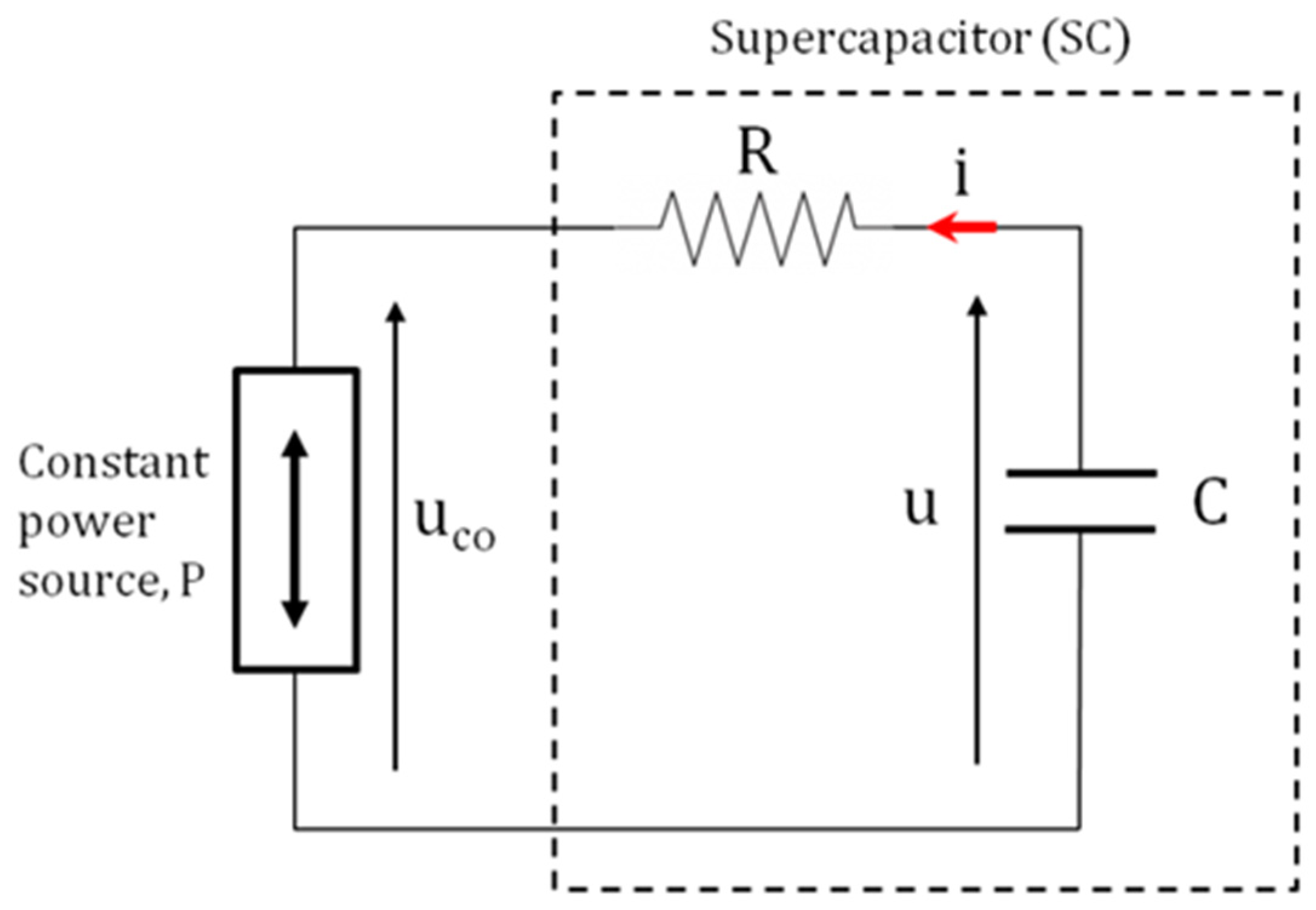
2.1. Electrical Analysis of an SC Cell Operating at Constant Power

A complete mathematical formulation for the electrical analysis of SCs operating at constant power is presented in [46] by the authors of this paper. Nevertheless, the main electrical variables involved in the charge and discharge of an SC cell at constant power will be hereafter described for the sake of clarity. As it can be seen in Figure 2, the cell is emulated by means of a RC-series electrical model, R being the internal resistance and C the rated capacitance, which is assumed to be constant. The remaining variables in Figure 2 are the internal voltage, u, the external voltage, u_co, and the discharge current, i.

The initial internal voltage of the cell is called ${\mathrm{U}}_0$. A discharge at constant power, P > 0, is assumed to begin at t = 0. From the mathematical formulation obtained in [46], a dimensionless variable, ${\mathrm{g}}_1\left(\mathrm{t}\right)$, can be defined as:

$${\mathrm{g}}_1\left(\mathrm{t}\right)=-{\mathrm{W}}_{-1}\left(\frac{-\exp (\frac{-\mathrm{g}(\mathrm{t})}{2·\mathrm{R}·\mathrm{P}})}{2·\mathrm{R}·\mathrm{P}}\right),$$

(1)

where ${\mathrm{W}}_{-1}\left(\mathrm{x}\right)$ is the secondary branch of the Lambert-W function. In the event of a charging process (P < 0), the main branch of the Lambert-W function, ${\mathrm{W}}_0\left(\mathrm{x}\right)$, must be used. The argument of this function includes another variable, $\mathrm{g}\left(\mathrm{t}\right)$, measured in V², that varies over time according to:

$$\mathrm{g}\left(\mathrm{t}\right)={\mathrm{U}}_0^2+{\mathrm{U}}_0·\sqrt{{\mathrm{U}}_0^2-4·\mathrm{R}·\mathrm{P}}-4·\mathrm{R}·\mathrm{P}·\ln \left({\mathrm{U}}_0+\sqrt{{\mathrm{U}}_0^2-4·\mathrm{R}·\mathrm{P}}\right)+2·\mathrm{R}·\mathrm{P}·\left[\ln \left(2\right)-1\right]-\frac{4·\mathrm{P}·\mathrm{t}}{\mathrm{C}}.$$

(2)

As is shown in this equation, the linear function $\mathrm{g}\left(\mathrm{t}\right)$ decreases over time for discharging processes and increases for charging. In order to obtain a clearer mathematical representation, it can be abbreviated as:

$$\mathrm{g}\left(\mathrm{t}\right)=\mathrm{A}-\frac{4·\mathrm{P}·\mathrm{t}}{\mathrm{C}},$$

(3)

where A is the y-intercept of $\mathrm{g}\left(\mathrm{t}\right)$,

$$\mathrm{A}={\mathrm{U}}_0^2+{\mathrm{U}}_0·\sqrt{{\mathrm{U}}_0^2-4·\mathrm{R}·\mathrm{P}}-4·\mathrm{R}·\mathrm{P}·\ln \left({\mathrm{U}}_0+\sqrt{{\mathrm{U}}_0^2-4·\mathrm{R}·\mathrm{P}}\right)+2·\mathrm{R}·\mathrm{P}·\left[\ln \left(2\right)-1\right].$$

(4)

As is detailed in [46], all the electrical variables involved in the analysis of the cell charge and discharge at constant power, as well as time, can be expressed as a function of ${\mathrm{g}}_1\left(\mathrm{t}\right)$. For instance, the power losses, ${\mathrm{p}}_{\mathrm{d}}$, in R can be calculated as:

$${\mathrm{p}}_{\mathrm{d}}=\frac{\mathrm{P}}{{\mathrm{g}}_1},$$

(5)

and the internal voltage, u, can be expressed as:

$$\mathrm{u}=\sqrt{\mathrm{R}·\mathrm{P}·{\mathrm{g}}_1}+\sqrt{\frac{\mathrm{R}·\mathrm{P}}{{\mathrm{g}}_1}}.$$

(6)

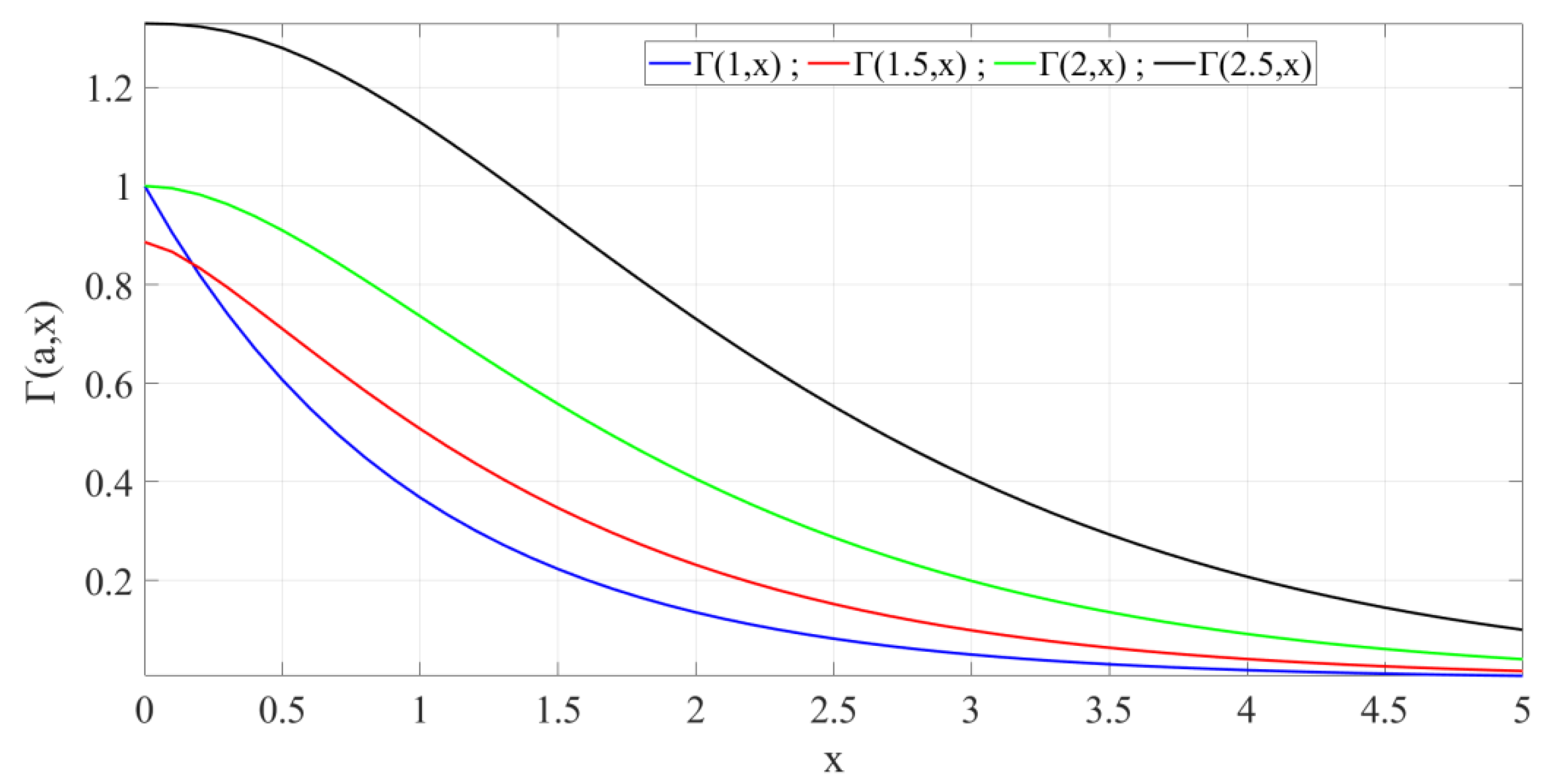
2.2. Incomplete Gamma Function

The incomplete Gamma Function is obtained from the gamma function, $\mathsf{\Gamma }\left(\mathrm{a}\right)$, which is defined as:

$$\mathsf{\Gamma }\left(\mathrm{a}\right)={\int }_0^{\infty }{\mathrm{t}}^{\mathrm{a}-1}·\exp \left(-\mathrm{t}\right)·\mathrm{dt},$$

(7)

where a > 0. The interval of integration of $\mathsf{\Gamma }\left(\mathrm{a}\right)$ can be split into two parts rendering two functions:

$$\mathsf{\gamma }\left(\mathrm{a},\mathrm{x}\right)={\int }_0^{\mathrm{x}}{\mathrm{t}}^{\mathrm{a}-1}·\exp \left(-\mathrm{t}\right)·\mathrm{dt},$$

(8)

$$\mathsf{\Gamma }\left(\mathrm{a},\mathrm{x}\right)={\int }_{\mathrm{x}}^{\infty }{\mathrm{t}}^{\mathrm{a}-1}·\exp \left(-\mathrm{t}\right)·\mathrm{dt},$$

(9)

where x ≥ 0. The functions γ(a, x) and Γ(a, x) are, respectively, called Lower and Upper Incomplete Gamma Functions. The latter being also called Complementary Incomplete Gamma Function or Prym’s function. Both are defined on complex numbers, but only on those with a positive real part in the case of γ(a, x). More specifically, the function Γ(a, x) will be used in this study to conduct the thermal analysis of the SC cell. In this regard, Figure 3 shows the evolution of Γ(a, x) for different values of a.

Another function,

$$\mathsf{\Gamma }\left(\mathrm{a},{\mathrm{x}}_1,{\mathrm{x}}_2\right)={\int }_{{\mathrm{x}}_1}^{{\mathrm{x}}_2}{\mathrm{t}}^{\mathrm{a}-1}·\exp \left(-\mathrm{t}\right)·\mathrm{dt}=\mathsf{\Gamma }\left(\mathrm{a},{\mathrm{x}}_1\right)-\mathsf{\Gamma }\left(\mathrm{a},{\mathrm{x}}_2\right),$$

(10)

called the Generalized Incomplete Gamma Function, can be defined from Γ(a, x) and is also used in this study. All the functions mentioned in this section are widely applied in other fields of research, such as astrophysics, probability theory, and engineering, particularly in heat transfer studies [57,58,59,60,61,62].

2.3. Thermal Analysis of SCs Operating at Constant Power Based on the Incomplete Gamma Function

The thermal model of the SC is based on the classical analogy with an electric circuit, as is shown in Figure 4 [33], where ${\mathrm{p}}_{\mathrm{d}}$ represents the power losses at the internal resistance of the cell, ${\mathrm{p}}_{\mathrm{amb}}$ stands for the heat power losses, ${\mathrm{T}}_{\mathrm{amb}}$ is the ambient temperature (considered constant), ${\mathrm{T}}_{\mathrm{cell}}$ is the temperature of the cell, ${\mathrm{p}}_{\mathrm{internal}}$ is the heat power that increases the thermal energy stored in the SC, and ${\mathrm{R}}_{\mathrm{TH}}$ [°C/W] and ${\mathrm{C}}_{\mathrm{TH}}$ [J/°C], respectively, are the thermal resistance and capacitance of the cell. Both ${\mathrm{R}}_{\mathrm{TH}}$ and ${\mathrm{C}}_{\mathrm{TH}}$ are usually provided by the manufacturer or can be calculated by conducting simple experimental tests.

The differential equation that determines the thermal behavior of the cell is as follows:

$${\mathrm{p}}_{\mathrm{d}}={\mathrm{C}}_{\mathrm{TH}}·\mathsf{\theta }\prime +\frac{\mathsf{\theta }}{{\mathrm{R}}_{\mathrm{TH}}},$$

(11)

$\mathsf{\theta }$ being the difference between the cell and ambient temperatures:

$$\mathsf{\theta }={\mathrm{T}}_{\mathrm{cell}}-{\mathrm{T}}_{\mathrm{amb}}.$$

(12)

Equation (11) can be expressed as a function of ${\mathrm{g}}_1$ by applying the chain rule:

$${\mathrm{p}}_{\mathrm{d}}={\mathrm{C}}_{\mathrm{TH}}·\frac{\mathrm{d}\mathsf{\theta }}{{\mathrm{dg}}_1}·\frac{{\mathrm{dg}}_1}{\mathrm{dt}}+\frac{\mathsf{\theta }}{{\mathrm{R}}_{\mathrm{TH}}}={\mathrm{C}}_{\mathrm{TH}}·\frac{\mathrm{d}\mathsf{\theta }}{{\mathrm{dg}}_1}·{\mathrm{g}}_1^{\prime }+\frac{\mathsf{\theta }}{{\mathrm{R}}_{\mathrm{TH}}}.$$

(13)

The time derivative of ${\mathrm{g}}_1$, ${\mathrm{g}}_1{}^{\prime }$, can be calculated by deriving Equation (1) and expressing the result as a function of ${\mathrm{g}}_1$ itself:

$${\mathrm{g}}_1{}^{\prime }=\frac{{\mathrm{dg}}_1}{\mathrm{dt}}=-\frac{2}{\mathrm{R}·\mathrm{C}}·\frac{{\mathrm{W}}_{-1}\left(\frac{-\exp \left(\frac{-\mathrm{g}\left(\mathrm{t}\right)}{2·\mathrm{R}·\mathrm{P}}\right)}{2·\mathrm{R}·\mathrm{P}}\right)}{1+{\mathrm{W}}_{-1}\left(\frac{-\exp \left(\frac{-\mathrm{g}\left(\mathrm{t}\right)}{2·\mathrm{R}·\mathrm{P}}\right)}{2·\mathrm{R}·\mathrm{P}}\right)}=\frac{2}{\mathrm{R}·\mathrm{C}}·\frac{{\mathrm{g}}_1}{1-{\mathrm{g}}_1}.$$

(14)

By combining Equations (5), (13) and (14), a first-order differential equation on $\mathsf{\theta }$ as a function of ${\mathrm{g}}_1$ can be obtained:

$$\frac{\mathrm{d}\mathsf{\theta }}{{\mathrm{dg}}_1}=\left(\frac{\mathrm{R}·\mathrm{C}}{2·{\mathrm{R}}_{\mathrm{TH}}·{\mathrm{C}}_{\mathrm{TH}}}\right)·\frac{{\mathrm{g}}_1-1}{{\mathrm{g}}_1}·\mathsf{\theta }-\left(\frac{\mathrm{R}·\mathrm{C}·\mathrm{P}}{2·{\mathrm{C}}_{\mathrm{TH}}}\right)·\frac{{\mathrm{g}}_1-1}{{\mathrm{g}}_1{}^2}.$$

(15)

In order to simplify Equation (15), a and b are defined as follows:

$$\mathrm{a}=\frac{\mathrm{R}·\mathrm{C}}{2·{\mathrm{R}}_{\mathrm{TH}}·{\mathrm{C}}_{\mathrm{TH}}}=\frac{\mathsf{\tau }}{2·{\mathsf{\tau }}_{\mathrm{TH}}},$$

(16)

$$\mathrm{b}=-\frac{\mathrm{R}·\mathrm{C}·\mathrm{P}}{2·{\mathrm{C}}_{\mathrm{TH}}}=-\frac{\mathsf{\tau }·\mathrm{P}}{2·{\mathrm{C}}_{\mathrm{TH}}},$$

(17)

where $\mathsf{\tau }$ and ${\mathsf{\tau }}_{\mathrm{TH}}$, respectively, are the electrical and thermal constants. Because in most commercial cells ${\mathsf{\tau }}_{\mathrm{TH}}$ ≫ $\mathsf{\tau }$, the value of a is within 0 and 1; 0 < a < 1. Moreover, as can be deduced from Equations (16) and (17), a is dimensionless, whereas b is measured in temperature units. These values can be assumed to be constant within the temperature range that goes from 0 °C to 65 °C because the electrical parameters of the cells, R and C, barely change in that span, as indicated by manufacturers [62,63], and P is assumed to be constant in this study. Therefore, Equation (15) can be expressed more compactly as:

$$\frac{\mathrm{d}\mathsf{\theta }}{{\mathrm{dg}}_1}=\left(\frac{{\mathrm{g}}_1-1}{{\mathrm{g}}_1}\right)·\left(\mathrm{a}·\mathsf{\theta }+\frac{\mathrm{b}}{{\mathrm{g}}_1}\right).$$

(18)

The general solution of Equation (18) is as follows:

$$\mathsf{\theta }\left({\mathrm{g}}_1\right)=\frac{\exp \left(\mathrm{a}·{\mathrm{g}}_1\right)}{{\mathrm{g}}_1{}^{\mathrm{a}}}·\left(\mathrm{k}+\frac{\mathrm{b}}{{\mathrm{a}}^{\mathrm{a}}}·\left(\mathrm{a}·\mathsf{\Gamma }\left(\mathrm{a}-1,\mathrm{a}·{\mathrm{g}}_1\right)-\mathsf{\Gamma }\left(\mathrm{a},\mathrm{a}·{\mathrm{g}}_1\right)\right)\right),$$

(19)

where k is the constant of integration, dependent on the initial temperature of the cell and $\mathsf{\Gamma }\left(\mathrm{a},\mathrm{x}\right)$ is the aforementioned Upper Incomplete Gamma Function. Considering the definition given for $\mathsf{\Gamma }\left(\mathrm{a},\mathrm{x}\right)$ in Equation (9) and integrating it by parts the following recursive expression can be defined:

$$\mathsf{\Gamma }\left(\mathrm{a}-1,\mathrm{a}·{\mathrm{g}}_1\right)=\left(\frac{1}{\mathrm{a}-1}\right)·\left(\mathsf{\Gamma }\left(\mathrm{a},\mathrm{a}·{\mathrm{g}}_1\right)-{\left(\mathrm{a}·{\mathrm{g}}_1\right)}^{\mathrm{a}-1}·\exp \left(-\mathrm{a}·{\mathrm{g}}_1\right)\right).$$

(20)

By replacing Equation (20) in Equation (19), and according to the definition of a and b given in Equations (16) and (17), the general solution of Equation (18) can be expressed as a function of the starting parameters, ${\mathrm{R}}_{\mathrm{TH}}$, P, and a, with the final solution being:

$$\mathsf{\theta }\left({\mathrm{g}}_1\right)={\left(\frac{\exp \left({\mathrm{g}}_1\right)}{{\mathrm{g}}_1}\right)}^{\mathrm{a}}·\left(\mathrm{k}-\frac{{\mathrm{R}}_{\mathrm{TH}}·\mathrm{P}}{{\mathrm{a}}^{\mathrm{a}-1}}·\left(\frac{1}{\mathrm{a}-1}\right)·\mathsf{\Gamma }\left(\mathrm{a},\mathrm{a}·{\mathrm{g}}_1\right)\right)+\frac{\mathrm{a}}{\left(\mathrm{a}-1\right)}·\frac{{\mathrm{R}}_{\mathrm{TH}}·\mathrm{P}}{{\mathrm{g}}_1}.$$

(21)

In the most general case, the cell will not initially be at the ambient temperature. In this situation for t = 0, ${\mathrm{g}}_1$ = ${\mathrm{g}}_{1\left(0\right)}$ and $\mathsf{\theta }\left({\mathrm{g}}_{1\left(0\right)}\right)$ = ${\mathsf{\theta }}_0$ =${\mathrm{T}}_0$ − ${\mathrm{T}}_{\mathrm{amb}}$, where ${\mathrm{T}}_0$ is the initial temperature of the cell and ${\mathrm{T}}_{\mathrm{amb}}$ the ambient temperature, are assumed to be constant, as explained above. Accordingly, Equation (21) can be solved for the constant of integration:

$$\mathrm{k}=({\mathsf{\theta }}_0+\frac{{\mathrm{R}}_{\mathrm{TH}}·\mathrm{P}·\mathrm{a}}{1-\mathrm{a}}·\frac{1}{{\mathrm{g}}_{1\left(0\right)}})·{\mathrm{g}}_{1\left(0\right)}{}^{\mathrm{a}}·\exp \left(-\mathrm{a}·{\mathrm{g}}_{1\left(0\right)}\right)+\frac{{\mathrm{R}}_{\mathrm{TH}}·\mathrm{P}}{{\mathrm{a}}^{\mathrm{a}-1}}·\left(\frac{1}{\mathrm{a}-1}\right)·\mathsf{\Gamma }\left(\mathrm{a},\mathrm{a}·{\mathrm{g}}_{1\left(0\right)}\right).$$

(22)

Finally, $\mathsf{\theta }$ can be expressed as a function of ${\mathrm{g}}_1$ by replacing k from Equation (22), in Equation (21):

$$\mathsf{\theta }\left({\mathrm{g}}_1\right)={\left(\frac{\exp \left({\mathrm{g}}_1\right)}{{\mathrm{g}}_1}\right)}^{\mathrm{a}}·\left({\mathrm{k}}_{\mathrm{T}1}+{\mathrm{k}}_{\mathrm{T}2}·\mathsf{\Gamma }\left(\mathrm{a},\mathrm{a}·{\mathrm{g}}_1\right)\right)+\frac{\mathrm{a}}{\left(\mathrm{a}-1\right)}·\frac{{\mathrm{R}}_{\mathrm{TH}}·\mathrm{P}}{{\mathrm{g}}_1}.$$

(23)

The new constants ${\mathrm{k}}_{\mathrm{T}1}$ and ${\mathrm{k}}_{\mathrm{T}2}$ have been defined, once more, to simplify the solution and are measured in temperature units:

$${\mathrm{k}}_{\mathrm{T}1}=({\mathsf{\theta }}_0+\frac{{\mathrm{R}}_{\mathrm{T}\mathrm{H}}·\mathrm{P}·\mathrm{a}}{1-\mathrm{a}}·\frac{1}{{\mathrm{g}}_{1(0)}})·{(\frac{{\mathrm{g}}_{1(0)}}{\exp ({\mathrm{g}}_{1(0)})})}^{\mathrm{a}}+\frac{{\mathrm{R}}_{\mathrm{T}\mathrm{H}}·\mathrm{P}}{{\mathrm{a}}^{\mathrm{a}-1}}·(\frac{1}{\mathrm{a}-1})·\Gamma (\mathrm{a},\mathrm{a}·{\mathrm{g}}_{1(0)}),$$

(24)

$${\mathrm{k}}_{\mathrm{T}2}=\frac{{\mathrm{R}}_{\mathrm{TH}}·\mathrm{P}}{{\mathrm{a}}^{\mathrm{a}-1}}·\left(\frac{1}{1-\mathrm{a}}\right).$$

(25)

As can be deduced, if the value of the electric constant $\mathsf{\tau }$ is much lower than the thermal constant: $\mathsf{\tau }\ll {\mathsf{\tau }}_{\mathrm{TH}}$, then a ≈ 0, ${\mathrm{k}}_{\mathrm{T}1}$ and ${\mathrm{k}}_{\mathrm{T}2}$ tend to ${\mathsf{\theta }}_0$ and 0, respectively, and the thermal jump $\mathsf{\theta }$ tends to ${\mathsf{\theta }}_0$, i.e., the temperature of the cell barely varies. This result is logical because the higher the thermal capacitance, the higher the thermal inertia and the lower the temperature increase with respect to the ambient for a given amount of power losses. The same happens if R tends to 0 because, in that case, a tends to 0 as well, and $\mathsf{\theta }$ maintains its initial value (${\mathsf{\theta }}_0$) since no thermal energy is dissipated.

By combining Equations (23)–(25), the thermal jump $\mathsf{\theta }$ can be alternatively expressed as:

$$\mathsf{\theta }\left({\mathrm{g}}_1\right)=\left({\mathsf{\theta }}_0+\frac{{\mathrm{R}}_{\mathrm{TH}}·\mathrm{P}·\mathrm{a}}{\left(1-\mathrm{a}\right)·{\mathrm{g}}_{1\left(0\right)}}\right)·{\left(\frac{{\mathrm{g}}_{1\left(0\right)}}{{\mathrm{g}}_1}·\frac{\exp \left({\mathrm{g}}_1\right)}{\exp \left({\mathrm{g}}_{1\left(0\right)}\right)}\right)}^{\mathrm{a}}+\frac{{\mathrm{R}}_{\mathrm{TH}}·\mathrm{P}·\mathrm{a}}{\left(\mathrm{a}-1\right)}·\left(\frac{\exp \left(\mathrm{a}·{\mathrm{g}}_1\right)·\mathsf{\Gamma }\left(\mathrm{a},\mathrm{a}·{\mathrm{g}}_{1\left(0\right)},\mathrm{a}·{\mathrm{g}}_1\right)}{{\left(\mathrm{a}·{\mathrm{g}}_1\right)}^{\mathrm{a}}}+\frac{1}{{\mathrm{g}}_1}\right),$$

(26)

where:

$$\mathsf{\Gamma }\left(\mathrm{a},\mathrm{a}·{\mathrm{g}}_{1\left(0\right)},\mathrm{a}·{\mathrm{g}}_1\right)=\mathsf{\Gamma }\left(\mathrm{a},\mathrm{a}·{\mathrm{g}}_{1\left(0\right)}\right)-\mathsf{\Gamma }\left(\mathrm{a},\mathrm{a}·{\mathrm{g}}_1\right),$$

(27)

according to Equation (10). A new function, $\mathrm{f}\left(\mathrm{a},{\mathrm{g}}_{1\left(0\right)},{\mathrm{g}}_1\right)$, and constants ${\mathrm{k}}_{\mathsf{\theta }1}$ and ${\mathrm{k}}_{\mathsf{\theta }2}$ can now be defined as:

$$\mathrm{f}\left(\mathrm{a},{\mathrm{g}}_{1\left(0\right)},{\mathrm{g}}_1\right)=\frac{\exp \left(\mathrm{a}·{\mathrm{g}}_1\right)·\mathsf{\Gamma }\left(\mathrm{a},\mathrm{a}·{\mathrm{g}}_{1\left(0\right)},\mathrm{a}·{\mathrm{g}}_1\right)}{{\left(\mathrm{a}·{\mathrm{g}}_1\right)}^{\mathrm{a}}}+\frac{1}{{\mathrm{g}}_1},$$

(28)

$${\mathrm{k}}_{\mathsf{\theta }1}=\left({\mathsf{\theta }}_0+\frac{{\mathrm{R}}_{\mathrm{TH}}·\mathrm{P}·\mathrm{a}}{\left(1-\mathrm{a}\right)·{\mathrm{g}}_{1\left(0\right)}}\right)·\exp \left(-\mathrm{a}·{\mathrm{g}}_{1\left(0\right)}\right),$$

(29)

$${\mathrm{k}}_{\mathsf{\theta }2}=\frac{{\mathrm{R}}_{\mathrm{TH}}·\mathrm{P}·\mathrm{a}}{\left(\mathrm{a}-1\right)},$$

(30)

in order to refine the result and defining a more compact and simple expression, we obtain:

$$\mathsf{\theta }\left({\mathrm{g}}_1\right)={\mathrm{k}}_{\mathsf{\theta }1}·{\left(\frac{{\mathrm{g}}_{1\left(0\right)}}{{\mathrm{g}}_1}\right)}^{\mathrm{a}}·\exp \left(\mathrm{a}·{\mathrm{g}}_1\right)+{\mathrm{k}}_{\mathsf{\theta }2}·\mathrm{f}\left(\mathrm{a},{\mathrm{g}}_{1\left(0\right)},{\mathrm{g}}_1\right).$$

(31)

Constants ${\mathrm{k}}_{\mathsf{\theta }1}$ and ${\mathrm{k}}_{\mathsf{\theta }2}$ are real numbers that are measured in temperature units, the former being positive in all the cases, and the latter being positive in charges (P < 0) and negative in discharges (P > 0).

The Incomplete Gamma Function, $\mathsf{\Gamma }\left(\mathrm{a},\mathrm{x}\right)$, provides real values when x ≥ 0 and complex numbers otherwise. Because the variable to be computed is a temperature, it cannot be a complex number. According to the definitions of ${\mathrm{g}}_1$ and its initial value, ${\mathrm{g}}_{1\left(0\right)}$, both of them are positive for discharges and negative for charges, as stated in [46]. Because a, according to Equation (16), is a non-integer positive real number, the functions $\mathsf{\Gamma }\left(\mathrm{a},\mathrm{a}·{\mathrm{g}}_1\right)$, $\mathsf{\Gamma }\left(\mathrm{a},\mathrm{a}·{\mathrm{g}}_{1\left(0\right)}\right)$ , and ${\left(\mathrm{a}·{\mathrm{g}}_1\right)}^{\mathrm{a}}$ render complex numbers for charge processes. However, the value of function $\mathrm{f}\left(\mathrm{a},{\mathrm{g}}_{1\left(0\right)},{\mathrm{g}}_1\right)$ is a real number in both charge and discharge. Taking into account that the incomplete Gamma Function, $\mathsf{\Gamma }\left(\mathrm{a},\mathrm{x}\right)$, can be expressed as a function of gamma function $\mathsf{\Gamma }\left(\mathrm{a}\right)$ as follows:

$$\mathsf{\Gamma }\left(\mathrm{a},\mathrm{x}\right)=\mathsf{\Gamma }\left(\mathrm{a}\right)-{\mathrm{x}}^{\mathrm{a}}·{\displaystyle \sum }_{\mathrm{k}=0}^{\infty }\frac{{\left(-\mathrm{x}\right)}^{\mathrm{k}}}{\left(\mathrm{a}+\mathrm{k}\right)·\mathrm{k}!}$$

(32)

it can be concluded, from Equation (10), that:

$$\frac{\mathsf{\Gamma }\left(\mathrm{a},\mathrm{a}·{\mathrm{g}}_{1\left(0\right)},\mathrm{a}·{\mathrm{g}}_1\right)}{{\left(\mathrm{a}·{\mathrm{g}}_1\right)}^{\mathrm{a}}}={\displaystyle \sum }_{\mathrm{k}=0}^{\infty }\frac{{\left(-\mathrm{a}·{\mathrm{g}}_1\right)}^{\mathrm{k}}}{\left(\mathrm{a}+\mathrm{k}\right)·\mathrm{k}!}-{\left(\frac{{\mathrm{g}}_{1\left(0\right)}}{{\mathrm{g}}_1}\right)}^{\mathrm{a}}·{\displaystyle \sum }_{\mathrm{k}=0}^{\infty }\frac{{\left(-\mathrm{a}·{\mathrm{g}}_{1\left(0\right)}\right)}^{\mathrm{k}}}{\left(\mathrm{a}+\mathrm{k}\right)·\mathrm{k}!}$$

(33)

Because the signs of ${\mathrm{g}}_1$ and ${\mathrm{g}}_{1\left(0\right)}$ are equal (both positive in discharges and both negative in charges), ${\left(\frac{{\mathrm{g}}_{1\left(0\right)}}{{\mathrm{g}}_1}\right)}^{\mathrm{a}}$ renders in Equation (33) a real number, as do both summations due to k being an integer. The same applies to the first summand in Equations (26) and (31). Finally, the temperature of the cell can be computed by summing the thermal jump $\mathsf{\theta }\left({\mathrm{g}}_1\right)$ in Equations (28)–(31) plus the ambient temperature:

$${\mathrm{T}}_{\mathrm{cell}}\left({\mathrm{g}}_1\right)=\mathsf{\theta }\left({\mathrm{g}}_1\right)+{\mathrm{T}}_{\mathrm{amb}}.$$

(34)

Once the temperature of the cell is expressed as a function of ${\mathrm{g}}_1$ (dimensionless), it can be defined as a function of the electrical variables involved in the charging and discharging processes (current, internal and external voltages, dissipated energy, state of charge, etc.) according to the expressions given in [46], or as a function of time from Equation (1). For instance, ${\mathrm{g}}_1$ can be expressed as a function of the external voltage as:

$${\mathrm{g}}_1=\frac{{\mathrm{u}}_{\mathrm{co}}^2}{\mathrm{R}·\mathrm{P}}.$$

(35)

By combining Equations (31), (34), and (35), the temperature of the cell can be expressed as a function of the external voltage as:

$${\mathrm{T}}_{\mathrm{cell}}\left({\mathrm{u}}_{\mathrm{co}}\right)={\mathrm{k}}_{\mathsf{\theta }1}·{\left(\frac{{\mathrm{u}}_{\mathrm{co}\left(0\right)}^2}{{\mathrm{u}}_{\mathrm{co}}^2}·\exp \left(\frac{{\mathrm{u}}_{\mathrm{co}}^2}{\mathrm{R}·\mathrm{P}}\right)\right)}^{\mathrm{a}}+{\mathrm{k}}_{\mathsf{\theta }2}·\mathrm{f}\left(\mathrm{a},\frac{{\mathrm{u}}_{\mathrm{co}\left(0\right)}^2}{\mathrm{R}·\mathrm{P}},\frac{{\mathrm{u}}_{\mathrm{co}}^2}{\mathrm{R}·\mathrm{P}}\right)+{\mathrm{T}}_{\mathrm{amb}},$$

(36)

where ${\mathrm{u}}_{\mathrm{co}\left(0\right)}$ represents the initial value of the external voltage, ${\mathrm{u}}_{\mathrm{co}}$. The same procedure can be repeated with any other variable involved in the process.

3. Discussion

The charge and discharge of an SC at both low and high constant power are assessed in this section in order to prove the proposed formulation valid. Parameters R, C, R_TH, and C_TH given by Maxwell Technologies™ for a 650-F cell are used [63] and shown in

Table 1. Parameters of the cell under study.

Electrical Values		Thermal Values			Constant
C (F)	R (mΩ)	${\mathbf{R}}_{\mathbf{T}\mathbf{H}} \left(°\mathrm{C}/\mathbf{W}\right)$	${\mathbf{C}}_{\mathbf{T}\mathbf{H}} \left(\mathbf{J}/°\mathrm{C}\right)$	${\mathbf{T}}_{\mathbf{a}\mathbf{m}\mathbf{b}} (°\mathrm{C})$	a
650	0.8	6.5	190	20	210.53 × 10−6

, which also includes the value of the constant a as defined in (16). Moreover, ${\mathrm{U}}_0$, P, ${\mathrm{T}}_0$, and ${\mathrm{T}}_{\mathrm{amb}}$ are assumed to be known variables as well.

The differential equation that enables the calculation of i can be defined by means of a power balance in the discharge:

$$0=-{\mathrm{i}}^3+\mathrm{C}·\left(\mathrm{P}-\mathrm{R}·{\mathrm{i}}^2\right)·\mathrm{i}\prime .$$

(37)

Three additional differential equations must be solved to compute the internal voltage u, the energy losses, ${\mathrm{e}}_{\mathrm{d}}$, and the thermal jump $\mathsf{\theta }$; once these variables are known, the other remaining electrical variables (external voltage, discharged energy, state of charge, etc.) can be calculated straightforwardly. These three equations are the well-known formula relating i and u, the relation between the power and energy losses, and the thermal Equation (11). Therefore, the equations system to be solved is as follows:

$$\{\begin{array}{c}\begin{array}{c}\mathrm{i}\prime =\frac{{\mathrm{i}}^3}{\mathrm{C}·\left(\mathrm{P}-\mathrm{R}·{\mathrm{i}}^2\right)}\\ \mathrm{u}\prime =-\frac{\mathrm{i}}{\mathrm{C}}\end{array}\\ {\mathrm{e}}_{\mathrm{d}}^{\prime }={\mathrm{p}}_{\mathrm{d}}=\mathrm{R}·{\mathrm{i}}^2\\ \theta \prime =\frac{\mathrm{R}·{\mathrm{i}}^2}{{\mathrm{C}}_{\mathrm{TH}}}-\frac{\mathsf{\theta }}{{\mathrm{R}}_{\mathrm{TH}·}{\mathrm{C}}_{\mathrm{TH}}}.\end{array}$$

(38)

As referred to above, once Equation (38) is solved, the thermal jump $\mathsf{\theta }$ and the other variables are directly obtained. All of them can be expressed as a function of the others.

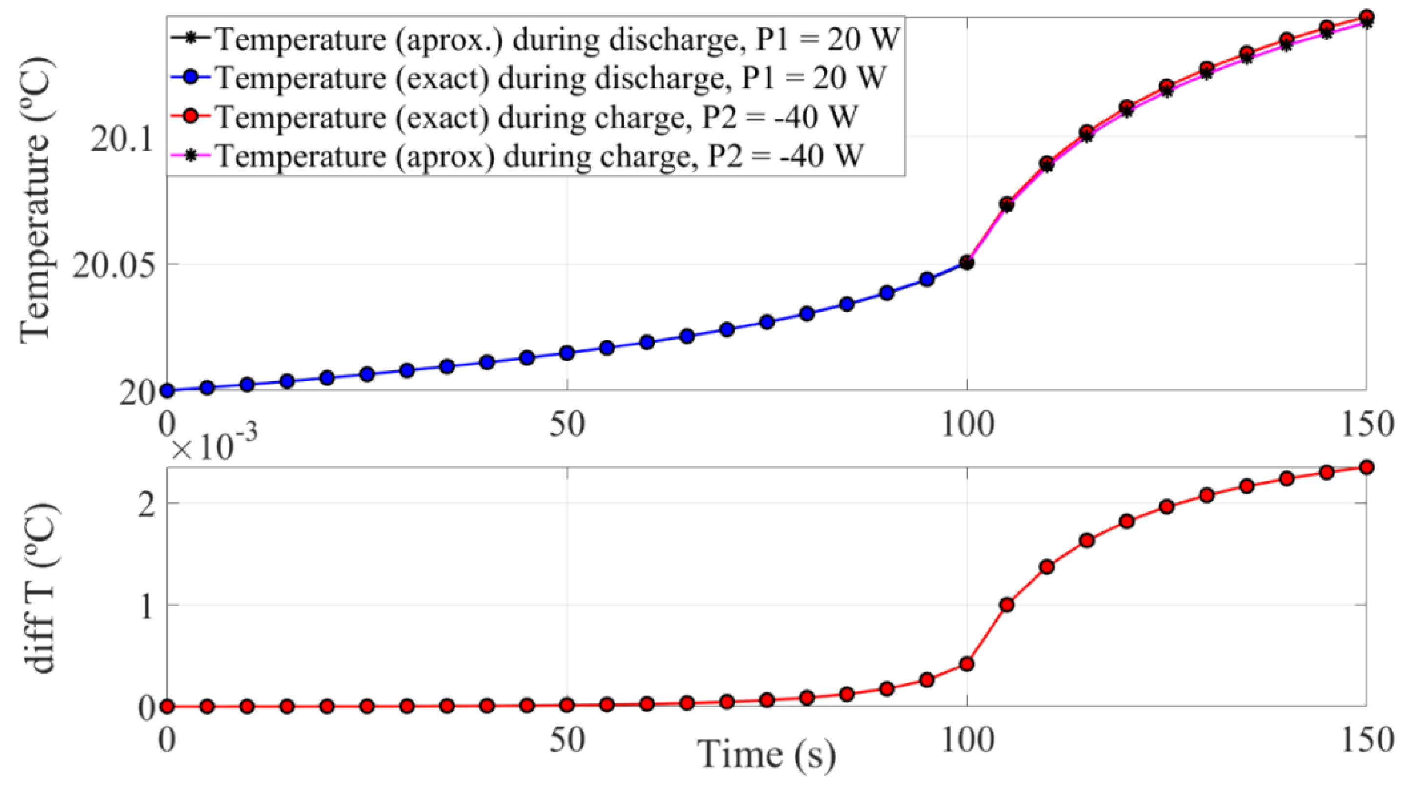
3.1. Charge and Discharge at Low Power

In this case study, the initial voltage of the cell is assumed to be 2.7 V. A discharge is followed by a charge. The former occurs at 20 W for 100 s, whereas the latter takes place at 40 W for 50 s. These values are below 4% of the maximum allowed power indicated by the manufacturer.

Table 2. Charge and discharge parameters at a low power.

With Proposed Formulas
Process	P (W)	Duration (s)	${\mathbf{T}}_0 (°\mathrm{C})$	${\mathbf{T}}_{\mathbf{f}\mathbf{i}\mathbf{n}\mathbf{a}\mathbf{l}} (°\mathrm{C})$	${\mathbf{U}}_0 \left(\mathbf{V}\right)$	${\mathbf{g}}_{1\left(0\right)}$	$k_{\mathsf{\theta }1}(°\mathrm{C})$	${\mathbf{k}}_{\mathsf{\theta }2}(°\mathrm{C})$
Discharge	20	100	20	20.05	2.7	453.623	54.849	−27.374
Charge	−40	50	20.05	20.15	1.0516	−36.528	52.419	54.748
With approximate formulas [56]
Discharge	20	100	20	20.047	2.7	-	-	-
Charge	−40	50	20.047	20.140	-	-	-	-
Difference (Diff T)
Discharge	20	100	0	4.168 × 10−4	-	-	-	-
Charge	−40	50	3 × 10−3	1 × 10−2	-	-	-	-

shows the values of the temperature at both the beginning and end of each time interval, as well as the internal voltage at the beginning of each process and the values of the constants ${\mathrm{g}}_{1\left(0\right)}$ (${\mathrm{g}}_1\left(\mathrm{t}\right)$ at t = 0), ${\mathrm{k}}_{\mathsf{\theta }1}$, and ${\mathrm{k}}_{\mathsf{\theta }2}$.

Figure 5 shows the temperature of the cell obtained every 5 s, by using both the formulas proposed in Section 2.3, and the approximate equations described in [56]. As can be concluded from the graph, the agreement between both formulations is absolute during the discharge, whereas a minor discrepancy can be observed during the charge. Therefore, the approximate equations practically provide the same results as those given by the proposed formulas, thus proving the former are proper for charging and discharging processes at low or moderate power values, as stated in [56].

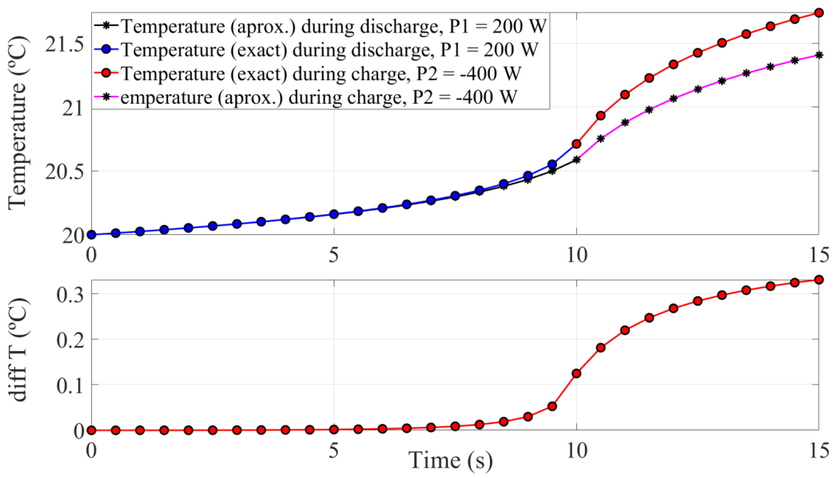
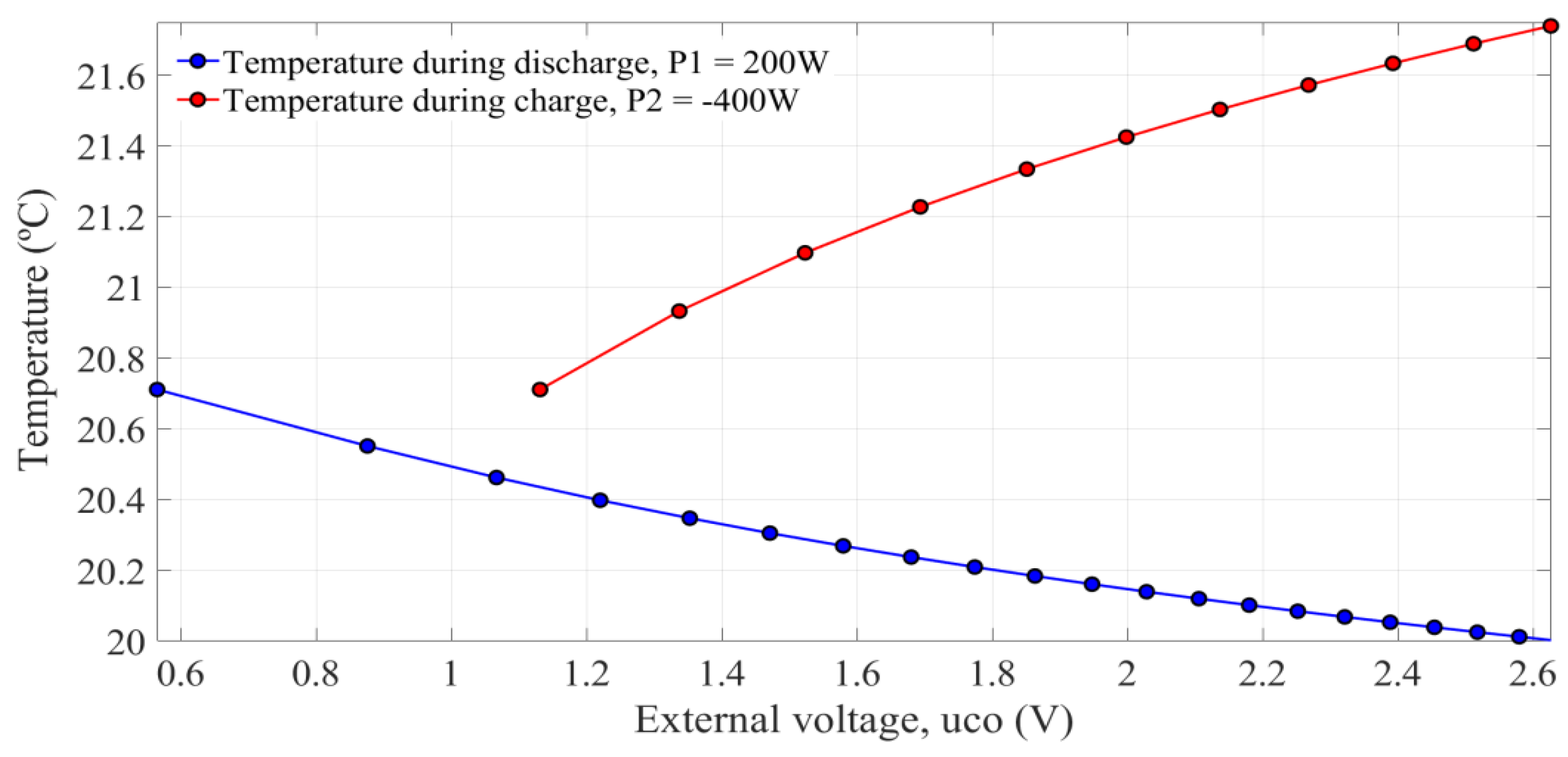
3.2. Charge and Discharge at High Power

In this case study, the initial voltage of the cell is also considered to be 2.7 V. A charge is preceded by a discharge as well. The discharge is assumed to occur at 200 W for 10 s, whereas the charge is kept at 400 W for 5 s. The latter is around 40% of the maximum allowed power given by the manufacturer, thus representing a high-power value.

Table 3. Charge and discharge parameters at a high power.

With Proposed Formulas
Process	P (W)	Duration (s)	${\mathbf{T}}_0 (°\mathrm{C})$	${\mathbf{T}}_{\mathbf{f}\mathbf{i}\mathbf{n}\mathbf{a}\mathbf{l}} (°\mathrm{C})$	${\mathbf{U}}_0 \left(\mathbf{V}\right)$	${\mathbf{u}}_{\mathbf{c}\mathbf{o}\left(0\right)} \left(\mathbf{V}\right)$	${\mathbf{g}}_{1\left(0\right)}$	${\mathbf{k}}_{\mathsf{\theta }1}(°\mathrm{C})$	${\mathbf{k}}_{\mathsf{\theta }2}(°\mathrm{C})$
Discharge	200	10	20	20.71	2.7	2.639	43.539	0.00623	−0.2737
Charge	−400	5	20.71	21.74	0.848	1.131	−3.998	0.84887	0.5475
With approximate formulas [56]
Discharge	200	10	20	20.59	2.7	-	-	-	-
Charge	−400	5	20.59	21.41	-	-	-	-	-
Difference (Diff T)
Discharge	200	10	0	0.12	2.7	-	-	-	-
Charge	−400	5	0.12	0.33	-	-	-	-	-

shows the data for this case, the external voltage at the beginning of each process, ${\mathrm{u}}_{\mathrm{co}\left(0\right)}$ has also been included. The electrical and thermal parameters of the cell are the ones presented in Table 1.

Figure 6 is the counterpart of Figure 5 for this case study. As can be observed, the results rendered by the approximate formulas diverge from the exact solution, more markedly during the charging process. Therefore, the exact formulation proposed in this study is the most suitable for high-power processes. It must be noticed that if more charge and discharge cycles were added after those 15 s, the accumulation of errors in each cycle would give rise to even greater differences between the approximate equations and the proposed exact solution.

Figure 7 shows the evolution of the variable ${\mathrm{g}}_1$ over time according to Equations (1) and (2). The values of ${\mathrm{g}}_1$ are positive during the discharge, whereas they are negative in the charge.

Figure 8 shows the evolution of the cell internal and external voltages over time according to Equations (1), (2), (6) and (35). The discontinuity that can be observed in the external voltage is due to the voltage drop at the internal resistance, as the reference of the current is reversed.

Figure 9 shows the evolution of the cell temperature as a function of the variable ${\mathrm{g}}_1$ obtained by means of Equations (28)–(34).

Figure 10 shows the evolution of the cell temperature as a function of the external voltage obtained from Equations (16), (28)–(30) and (36). As depicted in the graph, both variables increase during the charge, whereas the external voltage decreases and the temperature increases in the discharge.

3.3. Summary and Practical Application

A summary showing the procedure to obtain the temperature of an SC cell will be hereafter presented. The input data that define the SC will be the ones given by the manufacturer or those obtained in laboratory normalized tests: electrical resistance, R, capacitance, C, thermal resistance, R_TH, and thermal capacitance, C_TH. These are used together with the values of other variables, such as ambient temperature T_amb (assumed invariable), the initial value of the internal voltage, U₀, initial value of the cell temperature, T₀, and the charge or discharge power must be selected by the user, P.

To obtain the temperature of the cell vs. time, the process is the following:

• By means of the values of R, C, U₀, and P, the function g(t), described in the Equation (2), must be defined.
• Once g(t) is obtained, the function g₁(t) must be calculated by means of Equation (1).
• By using the values of R, C, R_TH, and C_TH, the constant “a” will be defined according to Equation (16).
• The initial thermal jump, θ₀, will be calculated as the difference between the initial temperature of the cell, T₀, and the ambient temperature, T_amb; θ₀ = T₀ − T_amb.
• Once θ₀, R_TH, P, a, and g₁₍₀₎ (g₁(t) for t = 0) are known, the value of the constants k_θ1 and k_θ2, according to the Equations (29) and (30), will be calculated. The function f(a, g₁₍₀₎, g₁) will be defined as well, as stated in Equation (28), g₁(t) being the function previously defined in the point 2 of this summary.
• The evolution of the temperature of the cell vs. time will be then the following:

$${\mathrm{T}}_{\mathrm{cell}}\left(\mathrm{t}\right)={\mathrm{k}}_{\mathsf{\theta }1}·{\left(\frac{{\mathrm{g}}_{1\left(0\right)}}{{\mathrm{g}}_1\left(\mathrm{t}\right)}\right)}^{\mathrm{a}}·\exp \left(\mathrm{a}·{\mathrm{g}}_1\left(\mathrm{t}\right)\right)+{\mathrm{k}}_{\mathsf{\theta }2}·\mathrm{f}\left(\mathrm{a},{\mathrm{g}}_{1\left(0\right),}{\mathrm{g}}_{1\left(\mathrm{t}\right)}\right)+{\mathrm{T}}_{\mathrm{amb}}$$

(39)

To express the temperature of the cell as a function of any other electrical variable, i.e., internal or external voltage, dissipated energy, etc., the process is nearly the same. Steps 1 and 2 should be omitted and g₁ should be defined as a function of the selected variable. If for the sake of clarity the desired variable is called “y”, the procedure is as simple as replacing g₁ by g₁(y); f(a, g₁₍₀₎, g₁) = f(a, g₁₍₀₎(y), g₁(y)) and with the f function; f(a, g₁₍₀₎(y), g₁(y)), the evolution of the temperature of the cell vs. y will be as follows:

$${\mathrm{T}}_{\mathrm{cell}}\left(\mathrm{y}\right)={\mathrm{k}}_{\mathsf{\theta }1}·{\left(\frac{{\mathrm{g}}_{1\left(0\right)}\left(\mathrm{y}\right)}{{\mathrm{g}}_1\left(\mathrm{y}\right)}\right)}^{\mathrm{a}}·\exp \left(\mathrm{a}·{\mathrm{g}}_1\left(\mathrm{y}\right)\right)+{\mathrm{k}}_{\mathsf{\theta }2}·\mathrm{f}\left(\mathrm{a},{\mathrm{g}}_{1\left(0\right)}\left(\mathrm{y}\right),{\mathrm{g}}_1\left(\mathrm{y}\right)\right)+{\mathrm{T}}_{\mathrm{amb}}.$$

(40)

This result has been obtained in the same way it was done in Equation (36) to calculate the temperature of the cell as function of the external voltage, u_co.

4. Conclusions

A set of formulas that enable the analytical calculation of the temperature of an SC cell subjected to charging and discharging processes at constant power have been presented. The traditional RC-series model has been used for both the electrical and thermal analysis. In this regard, the electrical and thermal parameters are normally provided by manufacturers or can be obtained by means of simple experimental tests. By applying the so-called Incomplete Gamma Function, the proposed formulation renders strictly accurate results for any operation mode (including high-power demand situations). This approach represents a breakthrough in the field of SCs because analytical results identical to those obtained by utilizing numerical methods are now provided. Therefore, the evolution of the cell temperature over time can be straightforwardly calculated from the cell parameters (electrical and thermal resistance and capacitance), charging and discharging power, the initial internal voltage and temperature, and the ambient temperature. Moreover, the cell temperature can be also expressed as a function of any other electrical variable (current, internal and external voltages, energy losses, state of charge, etc.), providing this way a useful and simple tool for designing, dimensioning, cooling, or developing new control algorithms.

References

1. Peng, H.; Wang, J.; Shen, W.; Shi, D.; Huang, Y. Compound control for energy management of the hybrid ultracapacitor-battery electric drive systems. Energy 2019, 175, 309–319. [Google Scholar] [CrossRef]
2. Joshi, M.C.; Samanta, S. Improved Energy Management Algorithm With Time-Share-Based Ultracapacitor Charging/Discharging for Hybrid Energy Storage System. IEEE Trans. Ind. Electron. 2019, 66, 6032–6043. [Google Scholar] [CrossRef]
3. Bolborici, V.; Dawson, F.P.; Lian, K.K. Hybrid Energy Storage Systems: Connecting Batteries in Parallel with Ultracapacitors for Higher Power Density. IEEE Ind. Appl. Mag. 2014, 20, 31–40. [Google Scholar] [CrossRef]
4. Zhao, C.; Yin, H.; Ma, C. Equivalent Series Resistance-based Real-time Control of Battery-Ultracapacitor Hybrid Energy Storage Systems. IEEE Trans. Ind. Electron. 2020, 67, 1999–2008. [Google Scholar] [CrossRef]
5. Zahedi, R.; Ardehali, M.M. Power management for storage mechanisms including battery, supercapacitor, and hydrogen of autonomous hybrid green power system utilizing multiple optimally-designed fuzzy logic controllers. Energy 2020, 204, 117935. [Google Scholar] [CrossRef]
6. Zeng, X.; Cui, C.; Wang, Y.; Li, G.; Song, D. Segemented Driving Cycle Based Optimization of Control Parameters for Power-Split Hybrid Electric Vehicle with Ultracapacitors. IEEE Access 2019, 7, 90666–90677. [Google Scholar] [CrossRef]
7. Lu, X.; Wang, H. Optimal Sizing and Energy Management for Cost-Effective PEV Hybrid Energy Storage Systems. IEEE Trans. Ind. Inform. 2020, 16, 3407–3416. [Google Scholar] [CrossRef]
8. Zhu, T.; Lot, R.; Wills, R.G.A.; Yan, X. Sizing a battery-supercapacitor energy storage system with battery degradation consideration for high-performance electric vehicles. Energy 2020, 208, 118336. [Google Scholar] [CrossRef]
9. Tao, F.; Zhu, L.; Fu, Z.; Si, P.; Sun, L. Frequency Decoupling-Based Energy Management Strategy for Fuel Cell/Battery/Ultracapacitor Hybrid Vehicle Using Fuzzy Control Method. IEEE Access 2020, 8, 166491–166502. [Google Scholar] [CrossRef]
10. Yue, X.; Kiely, J.; Gibson, D.; Drakakis, E.M. Charge-Based Supercapacitor Storage Estimation for Indoor Sub-mW Photovoltaic Energy Harvesting Powered Wireless Sensor Nodes. IEEE Trans. Ind. Electron. 2020, 67, 2411–2421. [Google Scholar] [CrossRef] [Green Version]
11. Palla, N.; Kumar, V.S.S. Coordinated Control of PV-Ultracapacitor System for Enhanced Operation under Variable Solar Irradiance and Short-Term Voltage Dips. IEEE Access 2020, 8, 211809–211819. [Google Scholar] [CrossRef]
12. Roy, P.; He, J.; Liao, Y. Cost Minimization of Battery-Supercapacitor Hybrid Energy Storage for Hourly Dispatching Wind-Solar Hybrid Power System. IEEE Access 2020, 8, 210099–210115. [Google Scholar] [CrossRef]
13. Aktaş, A.; Kırçiçek, Y. A novel optimal energy management strategy for offshore wind/marine current/battery/ultracapacitor hybrid renewable energy system. Energy 2020, 199, 117425. [Google Scholar] [CrossRef]
14. Yang, B.; Wang, J.; Sang, Y.; Yu, L.; Shu, H.; Li, S.; He, T.; Yang, L.; Zhang, X.; Yu, T. Applications of supercapacitor energy storage systems in microgrid with distributed generators via passive fractional-order sliding-mode control. Energy 2019, 187, 115905. [Google Scholar] [CrossRef]
15. Bhosale, R.; Agarwal, V. Fuzzy Logic Control of the Ultracapacitor Interface for Enhanced Transient Response and Voltage Stability of a DC Microgrid. IEEE Trans. Ind. Appl. 2019, 55, 712–720. [Google Scholar] [CrossRef]
16. Di Noia, L.P.; Genduso, F.; Miceli, R.; Rizzo, R. Optimal Integration of Hybrid Supercapacitor and IPT System for a Free-Catenary Tramway. IEEE Trans. Ind. Appl. 2019, 55, 794–801. [Google Scholar] [CrossRef]
17. Li, T.; Huang, L.; Liu, H. Energy management and economic analysis for a fuel cell supercapacitor excavator. Energy 2019, 172, 840–851. [Google Scholar] [CrossRef]
18. Mamun, A.; Liu, Z.; Rizzo, D.M.; Onori, S. An Integrated Design and Control Optimization Framework for Hybrid Military Vehicle Using Lithium-Ion Battery and Supercapacitor as Energy Storage Devices. IEEE Trans. Transp. Electrif. 2019, 5, 239–251. [Google Scholar] [CrossRef]
19. Macias, A.; Kandidayeni, M.; Boulon, L.; Trovão, J.P. Fuel cell-supercapacitor topologies benchmark for a three-wheel electric vehicle powertrain. Energy 2021, 224, 120234. [Google Scholar] [CrossRef]
20. Chen, H.; Zhang, Z.; Guan, C.; Gao, H. Optimization of sizing and frequency control in battery/supercapacitor hybrid energy storage system for fuel cell ship. Energy 2020, 197, 117285. [Google Scholar] [CrossRef]
21. Zhang, L.; Hu, X.; Wang, Z.; Sun, F.; Dorrell, D.G. A review of supercapacitor modeling, estimation, and applications: A control/management perspective. Renew. Sustain. Energy Rev. 2018, 81, 1868–1878. [Google Scholar] [CrossRef]
22. Marie-Francoise, J.; Gualous, H.; Berthon, A. Supercapacitor thermal- and electrical-behaviour modelling using ANN. IEEE Proc. Electr. Power Appl. 2006, 153, 255–262. [Google Scholar] [CrossRef]
23. Riu, D.; Retiere, N.; Linzen, D. Half-order modelling of supercapacitors. In Proceedings of the Conference Record of the 2004 IEEE Industry Applications Conference, 39th IAS Annual Meeting, Seattle, WA, USA, 3–7 October 2004; Volume 4, pp. 2550–2554. [Google Scholar] [CrossRef]
24. Martynyuk, V.; Ortigueira, M. Fractional model of an electrochemical capacitor. Signal Process. 2015, 107, 355–360. [Google Scholar] [CrossRef]
25. Sarwas, G.; Sierociuk, D.; Dzieliński, A. Ultracapacitor modeling and control with discrete fractional order artificial neural network. In Proceedings of the 13th International Carpathian Control Conference (ICCC), High Tatras, Podbanskě, Slovensko, 28–31 May 2012; pp. 617–622. [Google Scholar] [CrossRef]
26. Shi, L.; Crow, M.L. Comparison of ultracapacitor electric circuit models. In Proceedings of the 2008 IEEE Power and Energy Society General Meeting—Conversion and Delivery of Electrical Energy in the 21st Century, Pittsburgh, PA, USA, 20–24 July 2008; pp. 1–6. [Google Scholar] [CrossRef]
27. Zubieta, L.; Bonert, R. Characterization of double-layer capacitors for power electronics applications. IEEE Trans. Ind. Appl. 2000, 36, 199–205. [Google Scholar] [CrossRef] [Green Version]
28. Grbovic, P.J.; Delarue, P.; le Moigne, P.; Bartholomeus, P. Modeling and Control of the Ultracapacitor-Based Regenerative Controlled Electric Drives. IEEE Trans. Ind. Electron. 2011, 58, 3471–3484. [Google Scholar] [CrossRef]
29. Zhang, L.; Wang, Z.; Hu, X.; Sun, F.; Dorrell, D.G. A comparative study of equivalent circuit models of ultracapacitors for electric vehicles. J. Power Sources 2015, 274, 899–906. [Google Scholar] [CrossRef]
30. Zhang, Y.; Yang, H. Modeling and characterization of supercapacitors for wireless sensor network applications. J. Power Sources 2011, 196, 4128–4135. [Google Scholar] [CrossRef]
31. Devillers, N.; Jemei, S.; Péra, M.; Bienaimé, D.; Gustin, F. Review of characterization methods for supercapacitor modelling. J. Power Sources 2014, 246, 596–608. [Google Scholar] [CrossRef]
32. Miller, J.M. Ultracapacitor Applications; IET Power and Energy Series 59; The Institution of Engineering and Technology: London, UK, 2011; ISBN 9781849190718. [Google Scholar]
33. Grbovic, P.J. Ultra-Capacitors in Power Conversion Systems; IEEE Press: Piscataway, NJ, USA; Wiley: Hoboken, NJ, USA, 2013; ISBN 9781118356265. [Google Scholar]
34. Pedrayes, J.F.; Melero, M.G.; Cano, J.M.; Norniella, J.G.; Orcajo, G.A.; Cabanas, M.F.; Rojas, C.H. Optimization of supercapacitor sizing for high-fluctuating power applications by means of an internal-voltage-based method. Energy 2019, 183, 504–513. [Google Scholar] [CrossRef]
35. Gualous, H.; Louahlia-Gualous, H.; Gallay, R.; Miraoui, A. Supercapacitor Thermal Characterization in Transient State. In Proceedings of the IEEE Industry Applications Annual Meeting, New Orleans, LA, USA, 23–27 September 2007; pp. 722–729. [Google Scholar] [CrossRef]
36. Gualous, H.; Louahlia-Gualous, H.; Gallay, R.; Miraoui, A. Supercapacitor Thermal Modeling and Characterization in Transient State for Industrial Applications. IEEE Trans. Ind. Appl. 2009, 45, 1035–1044. [Google Scholar] [CrossRef]
37. Al Sakka, M.; Gualous, H.; van Mierlo, J.; Culcu, H. Thermal modeling and heat management of supercapacitor modules for vehicle applications. J. Power Sources 2009, 94, 581–587. [Google Scholar] [CrossRef]
38. Hijazi, A.; Kreczanik, P.; Bideaux, E.; Venet, P.; Clerc, G.; di Loreto, M. Thermal Network Model of Supercapacitors Stack. IEEE Trans. Ind. Electron. 2012, 59, 979–987. [Google Scholar] [CrossRef]
39. Rufer, A.; Barrade, P. A supercapacitor-based energy-storage system for elevators with soft commutated interface. IEEE Trans. Ind. Appl. 2002, 38, 1151–1159. [Google Scholar] [CrossRef]
40. Fouda, M.E.; Allagui, A.; Elwakil, A.S.; Eltawil, A.; Kurdahi, F. Supercapacitor discharge under constant resistance, constant current and constant power loads. J. Power Sources 2019, 435, 226829. [Google Scholar] [CrossRef]
41. Spyker, R.L.; Nelms, R.M. Analysis of double-layer capacitors supplying constant power loads. IEEE Trans. Aerosp. Electron. Syst. 2000, 36, 1439–1443. [Google Scholar] [CrossRef]
42. Barrade, P.; Rufer, A. Current Capability and Power Density of Supercapacitors: Considerations on Energy Efficiency. EPE J. 2003, 2, 4. [Google Scholar]
43. Miller, J.M. Electrical and Thermal Performance of the Carbon-carbon Ultracapacitor under Constant Power Conditions. In Proceedings of the 2007 IEEE Vehicle Power and Propulsion Conference, Arlington, TX, USA, 9–12 September 2007; pp. 559–566. [Google Scholar] [CrossRef]
44. Verbrugge, M.W.; Liu, P. Analytical Solutions and Experimental Data for Cyclic Voltammetry and Constant-Power Operation of Capacitors Consistent with HEV Applications. J. Electrochem. Soc. 2006, 153, A1237–A1245. [Google Scholar] [CrossRef]
45. Burke, A.F. Electrochemical capacitors. In Handbook on Batteries; UC Davis Institute of Transportation Studies: Davis, CA, USA, 2010. [Google Scholar]
46. Pedrayes, J.F.; Melero, M.G.; Cano, J.M.; Norniella, J.G.; Duque, S.B.; Rojas, C.H.; Orcajo, G.A.; Lambert, W. Function based closed-form expressions of supercapacitor electrical variables in constant power applications. Energy J. 2021, 218, 119364. [Google Scholar] [CrossRef]
47. Bittner, A.M.; Zhu, M.; Yang, Y.; Waibel, H.F.; Konuma, M.; Starke, U.; Weber, C.J. Ageing of electrochemical double layer capacitors. J. Power Sources 2012, 203, 262–273. [Google Scholar] [CrossRef]
48. Gualous, H.; Gallay, R.; Alcicek, G.; Tala-Ighil, B.; Oukaour, A.; Boudart, B.; Makany, P. Supercapacitor ageing at constant temperature and constant voltage and thermal shock. Microelectron. Reliab. 2010, 50, 1783–1788. [Google Scholar] [CrossRef]
49. Miller, J.R.; Butler, S. Capacitor system life reduction caused by cell temperature variation. In Proceedings of the Advanced Capacitor World Summit, San Diego, CA, USA, 17–19 July 2006. [Google Scholar]
50. Bohlen, O.; Kowal, J.; Sauer, D.U. Ageing behaviour of electrochemical double layer capacitors Part I. Experimental study and ageing model. J. Power Sources 2007, 172, 468–475. [Google Scholar] [CrossRef]
51. Bohlen, O.; Kowal, J.; Sauer, D.U. Ageing behaviour of electrochemical double layer capacitors Part II. Lifetime simulation model for dynalic applications. J. Power Sources 2007, 173, 626–632. [Google Scholar] [CrossRef]
52. Maxwell Technologies. Application Note, Life Duration Estimation. Available online: https://maxwell.com/wp-content/uploads/2021/08/applicationnote_1012839_1.pdf (accessed on 26 October 2021).
53. Murray, D.B.; Hayes, J.G. Cycle testing of supercapacitors for Long-Life Robust Applications. IEEE Trans. Power Electron. 2015, 30, 2505–2516. [Google Scholar] [CrossRef]
54. Schiffer, J.; Linzen, D.; Sauer, D.U. Heat generation in double layer capacitors. J. Power Sources 2006, 160, 765–772. [Google Scholar] [CrossRef]
55. Chiang, C.; Yang, J.; Cheng, W. Dynamic Modeling of the Electrical and Thermal Behavior of Ultracapacitors. In Proceedings of the 2013 IEEE International Conference on Control and Automation (ICCA), Hangzhou, China, 12–14 June 2013. [Google Scholar] [CrossRef]
56. Pedrayes, J.F.; Melero, M.G.; Norniella, J.G.; Cano, J.M.; Cabanas, M.F.; Orcajo, G.A.; Rojas, C.H. A novel analytical solution for the calculation of temperature in supercapacitors operating at constant power. Energy J. 2019, 188. [Google Scholar] [CrossRef]
57. Carslaw, H.S.; Jaeger, J.C. Conduction of Heat in Solids; Clarendon Press: Oxford, UK, 1992. [Google Scholar]
58. Zubair, S.M. Heat conduction in a semi-infinite solid subject to time-dependent surface heat fluxes: An analytical study. Wärme Stoffübertrag. 1993, 28, 357–364. [Google Scholar] [CrossRef]
59. Mehmetoglu, T. Use of Einstein-Debye method in the analytical and semi empirical analysis of isobaric heat capacity and thermal conductivity of nuclear materials. J. Nucl. Mater. 2019, 527, 151827, ISSN 0022-3115. [Google Scholar] [CrossRef]
60. Zhou, X.Y.; Yang, Z.Q.; Tang, X.R.; Wang, X.; Liu, Q.H. Fastest frozen temperature for a thermodynamic system. Results Phys. 2020, 18, 103153, ISSN 2211-3797. [Google Scholar] [CrossRef]
61. Mamedov, B.A. Analytical evaluation of the relativistic thermodynamic functions using binomial expansion theorem and incomplete Gamma functions. New Astron. 2012, 17, 353–355, ISSN 1384-1076. [Google Scholar] [CrossRef]
62. Maxwell Technologies. Document Number: 1013793.5. Maxwell Technologies, San Diego, CA, USA. Available online: https://www.mouser.com/datasheet/2/257/datasheet_hc_series_1013793-1640.pdf (accessed on 26 October 2021).
63. Maxwell Technologies. Datasheet—K2 Series Ultracapacitors; Document #1015370.4; Maxwell Technologies: San Diego, CA, USA; Available online: https://www.google.com/url?sa=t&rct=j&q=&esrc=s&source=web&cd=&ved=2ahUKEwju1JPI1O7zAhWuzzgGHfqkCFoQFnoECAYQAQ&url=http%3A%2F%2Fwww.mouser.com%2Fds%2F2%2F257%2FDATASHEET_K2_SERIES_1015370-5547.pdf&usg=AOvVaw05AOkMz_cPgoe7RsMpegDc (accessed on 26 October 2021).
Figure 1. Actual and discretized power profiles.
Applsci 11 10153 g001
Figure 2. Discharge of an SC at constant power.
Applsci 11 10153 g002
Figure 3. Upper Incomplete Gamma Function for different values of a.
Applsci 11 10153 g003
Figure 4. Thermal model of an SC based on an analogy with an electrical circuit.
Applsci 11 10153 g004
Figure 5. Top chart: Temperature of the cell obtained by using Equations (28)–(34) and the approximate equations given in [56] for discharge and charge at low or moderate power. Bottom chart: Temperature difference between both solutions.
Applsci 11 10153 g005
Figure 6. Top chart: Temperature of the cell obtained by using Equations (28)–(34) and the approximate equations given in [56] for discharge and charge at high power. Bottom chart: Temperature difference between both solutions.
Applsci 11 10153 g006
Figure 7. Evolution of variable g 1 over time.
Applsci 11 10153 g007
Figure 8. Evolution of the cell internal and external voltages over time.
Applsci 11 10153 g008
Figure 9. Evolution of the cell temperature as a function of the variable g 1 .
Applsci 11 10153 g009
Figure 10. Evolution of the cell temperature as a function of the external voltage.
Applsci 11 10153 g010