
A Novel Excitation Approach for Power Transformer Simulation Based on Finite Element Analysis


Department of Electrical Engineering, National Taiwan University of Science and Technology, Taipei 106, Taiwan
*
Author to whom correspondence should be addressed.
Appl. Sci. 2021, 11(21), 10334; https://doi.org/10.3390/app112110334
Submission received: 8 October 2021
/
Revised: 30 October 2021
/
Accepted: 1 November 2021
/
Published: 3 November 2021
Abstract
:Power transformers play an indispensable component in AC transmission systems. If the operating condition of a power transformer can be accurately predicted before the equipment is operated, it will help transformer manufacturers to design optimized power transformers. In the optimal design of the power transformer, the design value of the magnetic flux density in the core is important, and it affects the efficiency, cost, and life cycle. Therefore, this paper uses the software of ANSYS Maxwell to solve the instantaneous magnetic flux density distribution, core loss distribution, and total iron loss of the iron core based on the finite element method in the time domain. In addition, a new external excitation equation is proposed. The new external excitation equation can improve the accuracy of the simulation results and reduce the simulation time. Finally, the three-phase five-limb transformer is developed, and actually measures the local magnetic flux density and total core loss to verify the feasibility of the proposed finite element method of model and simulation parameters.
1. Introduction
Transformer manufacturers design power transformers based on factors such as insulation, efficiency, and cooling systems. In the optimal design of the transformer, it is necessary to consider the technical specifications, material costs, manufacturing costs, and capitalization costs [1,2]. Therefore, the design of the transformer involves multiphysics coupling and cost functions. It is difficult to find the best solution in limited time. If the operating conditions of the transformer can be predicted faster and accurately, the optimal design can be optimized. In [3], the three-phase five-leg wound power transformer was tested. The local magnetic flux density of the inner and outer corners, yokes, and limbs of the iron core was measured. The results show that the magnetic flux density of the outer corner, yoke, and limb is lower than that of the inner corner, yoke, and limb in the iron core. In [4], the magnetic field distribution of the U-type transformer was simulated based on the finite element method under different air gaps. In [5,6], the evolutionary algorithms combined with the finite element method were used to optimize the design of transformers. There are genetic algorithms (GA), differential evolution algorithms (DEA), and non-dominated sorting genetic algorithms (NSGA-II). The results showed that the design size of the core magnetic flux density affects the efficiency, total cost, and life cycle in the transformer. In [7], simulation software ANSYS Maxwell and ANSYS Mechanical were used to simulate the total iron loss and temperature of a three-phase five-limb power transformer with a capacity of 325 MVA. The simulation results were used to check the cooling system of the design in the transformer. In [8], the magnetic flux distortion of the three-phase five-limb transformer with direct current was analyzed based on the finite element analysis method. In [9], the magnetic field distribution and temperature distribution of three-phase three-limbed transformers were simulated based on the finite element method under DC bias. In [10], the local magnetic field distribution and eddy current loss with direct current offset were analyzed based on the circuit model and magnetic circuit model. The results showed that the peak magnetic flux density of the iron core will increase during the half-cycle under the DC bias, which is likely to cause vibration and local overheating of the transformer. In [11,12,13,14], scholars performed model fitting and research on the stray loss of transformers based on the finite element method. In [15], the stray loss of the high-frequency transformer was simulated based on the spectral element method.
According to the above applications, the magnetic flux density of the iron core in the transformer was studied. However, research on finite element analysis of fitting models is still lacking in the three-phase five-limb transformer. Therefore, this paper uses the software of ANSYS Maxwell to simulate the three-phase five-limb transformer in the time domain. The finite element model considers factors such as the structure of the iron core, the non-linear characteristics of the material, and the external excitation. The simulation results calculate the instantaneous magnetic flux density distribution and total core loss. The prototype of the three-phase five-limb transformer is measured to verify the proposed fitting model. Moreover, this paper studies the method of external excitation, which improves the accuracy of the simulation results. Finally, the proposed finite element analysis model will help transformer manufacturers reduce costs and improve efficiency and reliability in three-phase five-limb transformers.
2. 2D Finite Element Analysis Model
2.1. ANSYS Maxwell Solver Equation
The software of ANSYS Maxwell uses four Maxwell equations, which can be written as:
In Equations (1)–(4):
- B: magnetic flux density (T);
- H: magnetic field intensity (A/m);
- E: electric field (V/m);
- D: electric displacement (C/m2);
- J: conduction-current density (A/m2);
- : charge density (C/m2).
2.2. Core Loss Model
The core loss model consists of hysteresis loss, eddy current loss, and excessive loss. Its equation can be written as:
The symbols in Equation (5) are defined as:
In Equations (6)–(8):
- Bm: magnetic flux density of the iron core;
- f0: operating frequency of the transformer;
- kh: coefficient of the hysteresis loss;
- kc: coefficient of the eddy current loss coefficient;
- ke: coefficient of the excessive loss.
The three loss coefficients are determined according to the selected material of the iron core. Therefore, the Equations (5)–(8) are combined to get Equation (9):
The symbols in Equation (9) are defined as:
The equation of the classic eddy current loss model can be written as:
The symbol is the conductivity of the iron core and the symbol is the thickness of the iron core in Equation (12). The least square of the method can be used to solve the k1 coefficient and k2 coefficient. Equation (13) can be written as:
In Equation (13):
- Pvi: i-th iron loss of the P-B loss curve in the iron core;
- Bvi: i-th magnetic flux density of the P-B loss curve in the iron core.
Equations (10), (12) and (13) can be solved for the hysteresis loss coefficient kh. Therefore, the hysteresis loss coefficient kh and the excessive loss coefficient ke can be written as:
2.3. External Excitation
The open circuit of the transformer is shown in Figure 1. The circuit is composed of external excitation voltage Vin, leakage inductance Lk, series resistance Rs, magnetizing inductance Lm, and parallel resistance Rp.
To simplify the analysis, some conditions are assumed, namely:
- The external exciting voltage Vin is the ideal voltage source;
- Parallel resistance Rp is bigger than the magnetizing reactance XLm;
- The turns ratio is defined as N = N1/N2;
- The secondary side circuit is open;
- The external excitation voltages are balanced in three phases.
Since the external excitation voltages are balanced in three phases, the external excitation voltage of each phase can be written as Equations (16)–(18), where Vpeak is the peak value of the external excitation voltage and is the initial angle of the source:
The excitation current of each phase is calculated by Figure 1 and Equations (16)–(18). The excitation current equation of each phase can be written as:
The Equations (19)–(21) are defined as follows:
According to Equations (16)–(18), the excitation current of each phase has AC steady-state components and DC transient components. When the AC steady-state component and the DC transient component are in the same square phase, the peak value of the exciting current will increase in the half-cycle. The peak value of the magnetic flux density is increased by this phenomenon. This will cause the iron core to enter the saturation region when the phenomenon is serious. Therefore, the slow start function is added to the equation of the external excitation voltage to avoid magnetic flux density deviation in the iron core. Therefore, the equations have been proposed by scholars, and the equations can be written as Equations (24)–(26) [7,16], where is the slow start parameter:
According to Equations (24)–(26), the slow start parameter is constant. The simulation time is short and the accuracy of the simulation is lower under a big slow start parameter. Conversely, the simulation time is longer and the accuracy of the simulation is higher under the small slow start parameter. However, the small slow start parameter increases the time of each iteration in the coupling field, which consists of the magnetic field and the temperature field based on the sequential method. Therefore, this paper proposes the new external excitation voltage equation, in which the slow start function is the double exponential function. Comparing the conventional equation, the double exponential function makes the slow start parameter change over time. In the beginning, the slow start parameter is small. The slow start parameter becomes larger as the simulation time progresses. The proposed external excitation voltage equation of each phase can be written as Equations (27)–(29), where is the slow start parameter:
2.4. 2D Model Depth
Since the actual model of the iron core is not a rectangular parallelepiped, it is necessary to calculate the 2D model depth of the core to restore the actual model. If the insulation film of the iron core is not considered, the 2D model depth equation can be written as:
3. Finite Element Analysis Simulation
3.1. Simulation Model
The 2D model of a three-phase five-limb transformer is shown in Figure 2. The model is composed of the exciting coil, the iron core, and the test environment. The model of the iron core has a gap.
In actual transformers, the iron core has a certain thickness. The 2D simulation model has no third dimension to establish the thickness of the iron core. Therefore, the 2D model depth is added to the 2D simulation model. The 2D model depth makes the equivalent total volume of the simulation iron core model the same as the total volume of the actual iron core model. According to the iron core of the experimental model, the cross-section area of the single limb is 4960.992 mm2. The length of the iron core is 480 mm in the simulation model. The 2D model depth is 10.3354 mm, which is calculated by the Equation (30). The parameters of the simulation model as shown in Table 1.
The materials of the simulation model are defined before simulating iron loss and magnetic flux density. The materials of the simulation model are shown in Table 2. The material items are the excitation coil, iron core, gap, and environment.
The non-linear factors of the iron core are considered. The B-H curve of the iron core is shown in Figure 3. The P-B curve of the iron core is shown in Figure 4.
The thickness of the iron core is considered, and its value is 0.27 mm. The loss coefficients of the iron core are calculated by the P-B curve, mass density, thickness, and operating frequency in the iron core. Therefore, they are calculated from Equations (5)–(15), Table 2, and Figure 4, as shown in Table 3.
3.2. External Excitation Parameters
The parameters of the external excitation voltage equations are shown in Table 4. The slow start parameter of conventional equations was defined as 50 in previous research [7,16]. In order to improve the accuracy of the simulation results, the slow start parameter of conventional equations is defined as 5 in this paper. The slow start parameters of the proposed equations are defined in four groups, i.e., 25, 50, 75, and 100. Moreover, the turn numbers of each phase are 46 turns and the resistance of each phase is 1.5708 µΩ in the excitation coil.
3.3. Simulation Results
The eddy current effect is not considered in the winding. The simulation results of the winding voltage without a slow start are shown in Figure 5. The simulation results of the winding voltage under conventional equations with an external excitation voltage are shown in Figure 6. The simulation results of the winding voltage under the proposed equations of the external excitation voltage are shown in Figure 7. The peak voltage of each phase is 301.64 V.
The simulation results of the winding flux linkage without a slow start are shown in Figure 8, and its deviation is 75%. Moreover, the simulation results of the winding flux linkage under conventional external excitation equations are shown in Figure 9. When and , the winding flux linkage deviation is 20.7% and 2.325%, respectively. The simulation results of winding flux linkage under the proposed external excitation equation are shown in Figure 10. When , , , and , the winding flux linkage deviations are 0.387%, 0.312%, 1.043%, and 5.87%, respectively.
The simulation results of the core loss without a slow start are shown in Figure 11. The simulation results of the core loss under conventional external excitation equations are shown in Figure 12. The simulation results of the core loss under the proposed external excitation equation are shown in Figure 13. The average core losses under different slow start functions are shown in Table 5. The total core loss is composed of two loss components, which are the eddy current loss component and the hysteresis loss component. The average interval time is 200 ms. According to Figure 6, when the and , the time for the external excitation voltage to reach the steady-state is 0.08 s and 0.98 s, respectively. According to Figure 7, when the , , , and , the time for the external excitation voltage to reach steady-state is 0.04 s, 0.06 s, 0.08 s, and 0.14 s, respectively. Therefore, the average interval is 80 ms to 100 ms under , , , and and no slow start condition. The average interval is 0.98 s to 1 s under . The average interval is 0.14 s to 0.16 s under .
The simulation results of the magnetic flux density distribution under different external excitation voltage functions are shown in Figure 14. The calculation method is the average magnetic flux density of the cross-section area of the iron core in the steady-state, and it is the maximum value at a moment in a cycle.
The magnetic flux density of the medium limb is 2.64275 T under the no slow start condition. According to the conventional equations, when and , the magnetic flux density of the medium limb is 1.9534 T and 1.75345 T, respectively. According to the proposed equations, when , , , and , the magnetic flux density of the medium limb is 1.7445 T, 1.7393 T, 1.75635 T, and 1.82085 T, respectively. The simulation results show that the magnetic flux density of the inner iron core is bigger than the magnetic flux density of the outer iron core under different external excitation functions.
4. Experimental Results
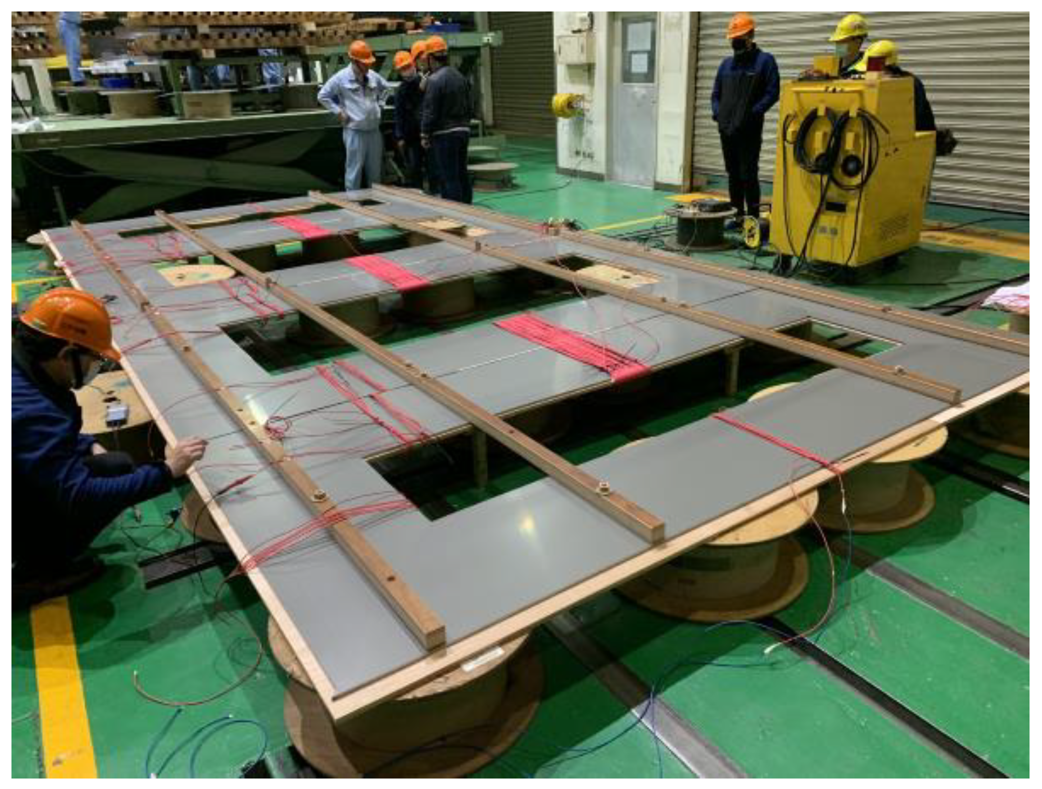
This chapter uses the simulation results from simulation software ANSYS Maxwell and the experimental results to verify the proposed finite element analysis model. First, the adjustable AC power supply is applied to the three-phase five-limb transformer. Secondly, the induced electromotive force is measured by the test coil. Finally, the magnetic flux density of the iron core is calculated according to Faraday’s law. The setting diagram of the three-phase five-limb transformer is shown in Figure 15, in which the test coils S1–S12 are single yokes and single limbs, and the test coils S13–S15 are all limbs. The external voltage is 213.33 V, and the operating frequency is 60 Hz. The turn number of the excitation coil is 46 turns, and the turn number of the test coil is 6 turns. The measured three-phase five-limb is shown in Figure 16.
The experimental results of the magnetic flux density under different test coils are shown in Table 6. The magnetic flux density of medium limb S14 is 1.6884 T. Compared with the simulation results without a slow start, the error is 56.52%. Compared with the simulation results of the convention equation, when and , the error is 15.69% and 4.45%, respectively. Compared with the simulation results of the proposed equation, when , , , and , the error is 3.33%, 4.19%, 4.02%, and 7.84%, respectively. The structure of the three-phase five-limb transformer is symmetrical. When the simulation result of the magnetic flux density is good in the middle limbs, the simulation results of other local limbs and yokes are better. Therefore, the middle limb of the simulation result is the best under the proposed equation. When the proposed equation , the interlimb S10 error is 2.6%, the outer limb S1 error is 7.92%, the internal yoke S3 error is 5.28%, and the outer yoke S2 error is 7.51%. According to the experimental results and simulation results, the magnetic flux density of the inner iron core is bigger than the magnetic flux density of the outer iron core.
The experimental results of the core loss are shown in Table 7. The measured core loss is 1.949 kW. Compared with the simulation results without slow start, the error is 23.61%. Compared with the simulation results of the convention equation, when and , the error is 0.28% and 6.12%, respectively. Compared with the simulation results of the proposed equation, when , , , and , the error is 0.056%, 0.743%, 1.452%, and 2.678%, respectively. Comparing the conventional equation under , the accuracy of simulation results is improved and simulation time is shortened by 6 times in the proposed equation with . If the simulation time is less than 0.1 s, the accuracy of core loss is increased by 31 times. The finite element model of the simulation is verified by Table 6 and Table 7. It is verified that the slow start function and parameter are important for the accuracy of the simulation results. The simulation results have not considered the harmonics. Therefore, the simulation results of the magnetic flux density distribution are slightly different from the experimental results of the magnetic flux density distribution.
5. Conclusions
This paper uses the finite element method to simulate the core loss and magnetic flux distribution of the iron core in the transformer. The finite element analysis model includes the iron loss model, equation of external excitation, and model depth. The iron loss model can be divided into three components: hysteresis loss, eddy current loss, and excessive loss. The non-linear factors of magnetic material are considered by the iron loss model. The non-linear factors include the B-H curve, P-B curve, conductivity, mass density, thickness, and operating frequency. The excitation current of each phase is composed of the steady-state AC component and the transient DC component in the equivalent open circuit. The magnetic density deviation is caused by the transient DC component. Therefore, the equation of external excitation voltage added the slow start function, which can avoid the magnetic deviation. The double exponential of the slow start function is proposed. Compared with the conventional external excitation equation, the new external excitation equation can improve the accuracy of simulation results and reduce the simulation time. According to the experimental results and simulation results, the error of core loss is 0.056%, and the error of medium limb magnetic density is 3.33% under= 25. The simulation time is reduced by 6 times. Therefore, the finite element analysis model is verified by the experimental results and simulation results. Finally, it can accurately predict the local magnetic flux density of the iron core when the transformer is in operation using the proposed finite element analysis model. The transformer manufacturers reduce costs and improve the efficiency and reliability in three-phase five-limb transformers.
Author Contributions
Conceptualization, W.-C.C. and C.-C.K.; methodology, W.-C.C.; software, W.-C.C.; validation, W.-C.C. and C.-C.K.; formal analysis, W.-C.C. and C.-C.K.; investigation, W.-C.C. and C.-C.K.; resources, W.-C.C. and C.-C.K.; data curation, W.-C.C. and C.-C.K.; writing—original draft preparation, W.-C.C.; writing—review and editing, C.-C.K. All authors have read and agreed to the published version of the manuscript.
Funding
This research received no external funding.
Institutional Review Board Statement
Not applicable.
Informed Consent Statement
Not applicable.
Data Availability Statement
All data are already provided in the manuscript.
Acknowledgments
Support for this research from Shihlin Electric is gratefully acknowledged.
Conflicts of Interest
The authors declare no conflict of interest.
References
- Orosz, T. Evolution and Modern Approaches of the Power Transformer Cost Optimization Methods. Period. Polytech. Electr. Eng. Comput. Sci. 2019, 63, 37–50. [Google Scholar] [CrossRef] [Green Version]
- Orosz, T.; Sleisz, Á.; Tamus, Z.Á. Metaheuristic Optimization Preliminary Design Process of Core-Form Autotransformers. IEEE Tran. Magn. 2016, 52, 1–10. [Google Scholar] [CrossRef]
- Loizos, G.; Kefalas, T.D.; Kladas, A.G.; Souflaris, A.T. Flux Distribution Analysis in Three-Phase Si-Fe Wound Transformer Cores. IEEE Tran. Magn. 2010, 46, 594–597. [Google Scholar] [CrossRef]
- Li, L.; Du, X.; Pan, J.; Keating, A.; Matthews, D.; Huang, H.; Zheng, J. Distributed Magnetic Flux Density on the Cross-Section of a Transformer Core. Electronics 2019, 8, 297. [Google Scholar] [CrossRef] [Green Version]
- Mohammed, M.S.; Vural, R.A. NSGA-II+FEM Based Loss Optimization of Three-Phase Transformer. IEEE Trans. Ind. Electron. 2019, 66, 7417–7425. [Google Scholar] [CrossRef]
- Orosz, T.; Pánek, D.; Karban, P. FEM Based Preliminary Design Optimization in Case of Large Power Transformers. Appl. Sci. 2020, 10, 1361. [Google Scholar] [CrossRef] [Green Version]
- Nicolae, P.M.; Constantin, D.; NITU, M.C. 2D Electromagnetic Transient and Thermal Modeling of a Three-Phase Power Transformer. In Proceedings of the 2013 4th International Youth Conference on Energy (IYCE), Siófok, Hungary, 6–8 June 2013; pp. 1–5. [Google Scholar] [CrossRef]
- Biro, O.; Buchgraber, G.; Leber, G.; Preis, K. Prediction of Magnetizing Current Wave-Forms in a Three-Phase Power Transformer Under DC Bias. IEEE Tran. Magn. 2008, 44, 1554–1557. [Google Scholar] [CrossRef]
- Gong, R.; Ruan, J.; Chen, J.; Quan, Y.; Wang, J.; Jin, S. A 3-D Coupled Magneto-Fluid-Thermal Analysis of a 220 kV Three-Phase Three-Limb Transformer under DC Bias. Energies 2017, 10, 422. [Google Scholar] [CrossRef]
- Xia, D. The Distribution of Transient Magnetic Field and Eddy Current Losses of Three-Phase Five-Legged Transformer under DC Bias. In Proceedings of the 2018 IEEE International Conference on Internet of Things (iThings) and IEEE Green Computing and Communications (GreenCom) and IEEE Cyber, Physical and Social Computing (CPSCom) and IEEE Smart Data (SmartData), Halifax, NS, Canada, 30 July 2018; pp. 728–732. [Google Scholar] [CrossRef]
- Smajic, J.; Steinmetz, T.; Cretu, B.C.; Nogues, A.; Murillo, R.; Tepper, J. Analysis of Near and Far Stray Magnetic Fields of Dry-Type Transformers: 3-D Simulations Versus Measurements. IEEE Tran. Magn. 2011, 47, 1374–1377. [Google Scholar] [CrossRef]
- Moghaddami, M.; Sarwat, A.I.; Leon, F.D. Reduction of Stray Loss in Power Transformers Using Horizontal Magnetic Wall Shunts. IEEE Tran. Magn. 2017, 53, 1374–1377. [Google Scholar] [CrossRef]
- Park, K.H.; Lee, H.J.; Hahn, S.C. Finite-Element Modeling and Experimental Verification of Stray-Loss Reduction in Power Transformer Tank with Wall Shunt. IEEE Tran. Magn. 2019, 55, 1–4. [Google Scholar] [CrossRef]
- Khan, S.; Maximov, S.; Escarela-Perez, R.; Olivares-Galvan, J.C.; Melgoza-Vazquez, E.; Lopez-Garcia, I. Computation of Stray Losses in Transformer Bushing Regions Considering Harmonics in the Load Current. Appl. Sci. 2020, 10, 3527. [Google Scholar] [CrossRef]
- Bastiaens, K.; Curti, M.; Krop, D.C.J.; Jumayev, S.; Lomonova, E.A. Spectral Element Method Modeling of Eddy Current Losses in High-Frequency Transformers. Math. Comput. Appl. 2019, 24, 28. [Google Scholar] [CrossRef] [Green Version]
- Bal, S.; Demirdelen, T.; Tümay, M. Three-Phase Distribution Transformer Modeling and Electromagnetic Transient Analysis Using ANSYS Maxwell. In Proceedings of the 2019 3rd International Symposium on Multidisciplinary Studies and Innovative Technologies (ISMSIT), Ankara, Turkey, 11–13 October 2019. [Google Scholar] [CrossRef]
Figure 1.
The open circuit of the transformer diagram.

Figure 2.
2D simulation model diagram.

Figure 3.
The B-H curve of the iron core diagram.
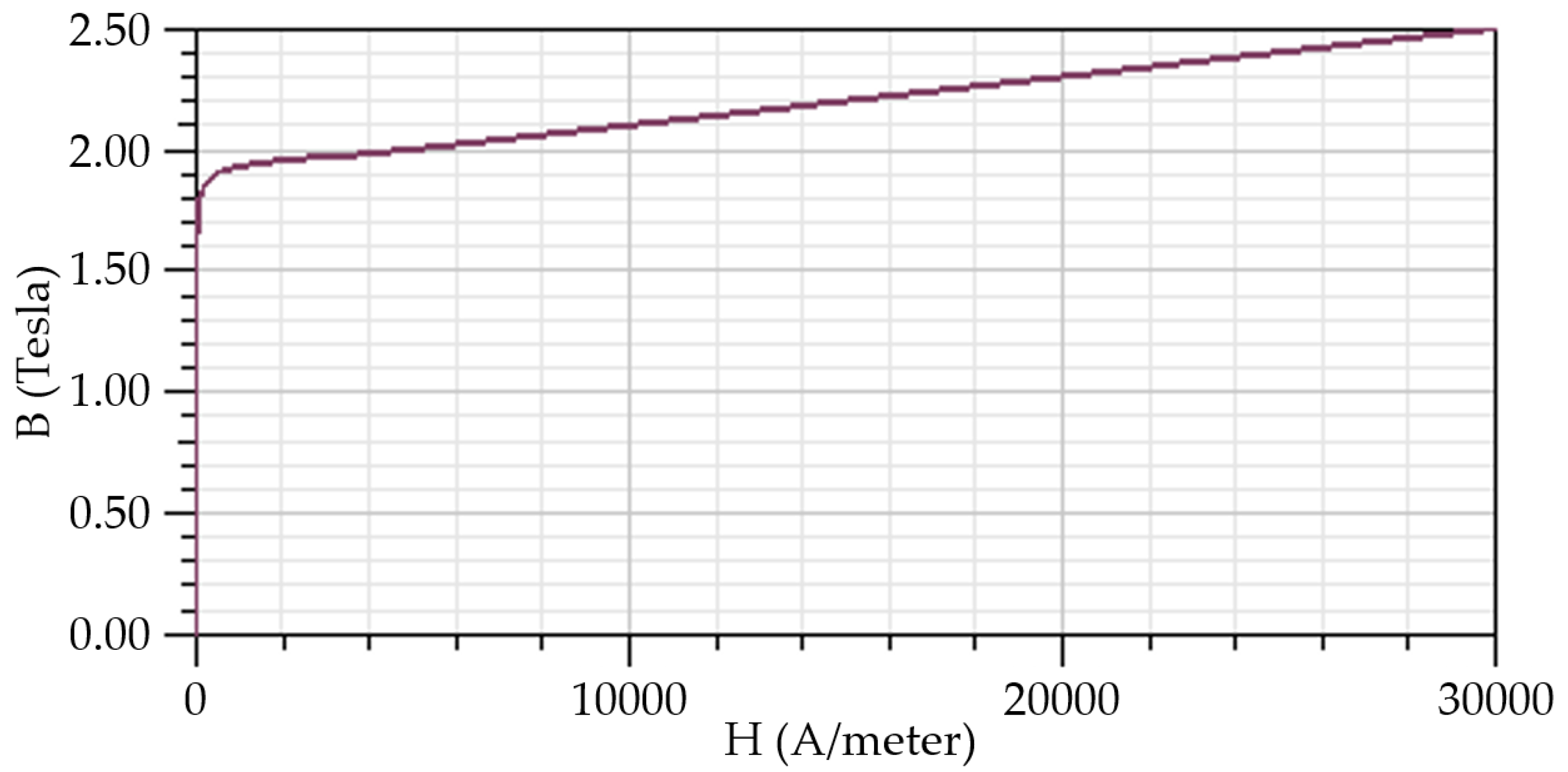
Figure 4.
The P-B curve of the iron core diagram.
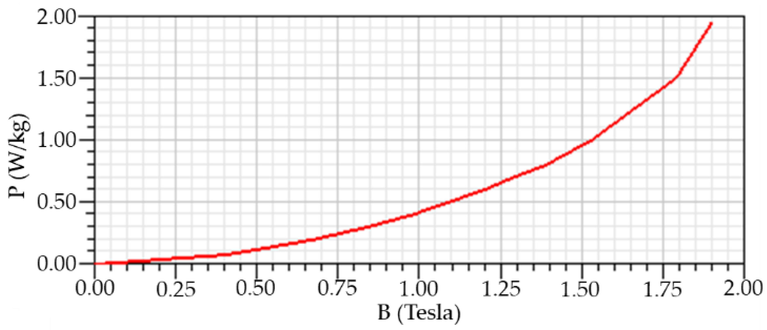
Figure 5.
Simulation results of the winding voltage without a slow start.

Figure 6.
Simulation results of the winding voltage under the conventional equation. (a) ; (b) .
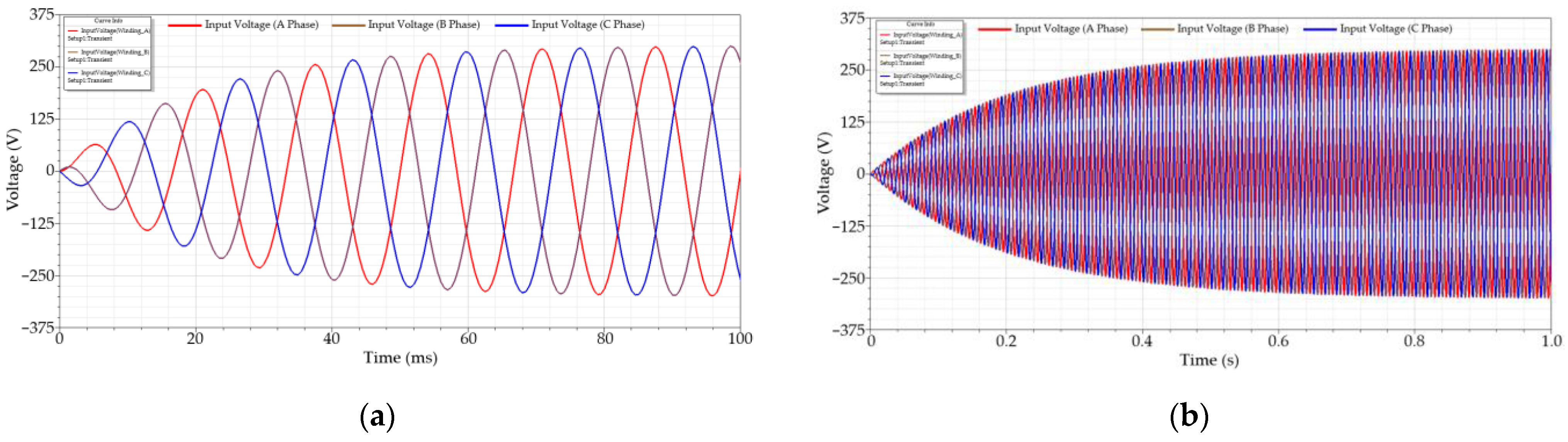
Figure 7.
Simulation results of the winding voltage under the proposed equation. (a) ; (b) ; (c) ; (d) .
Figure 7.
Simulation results of the winding voltage under the proposed equation. (a) ; (b) ; (c) ; (d) .
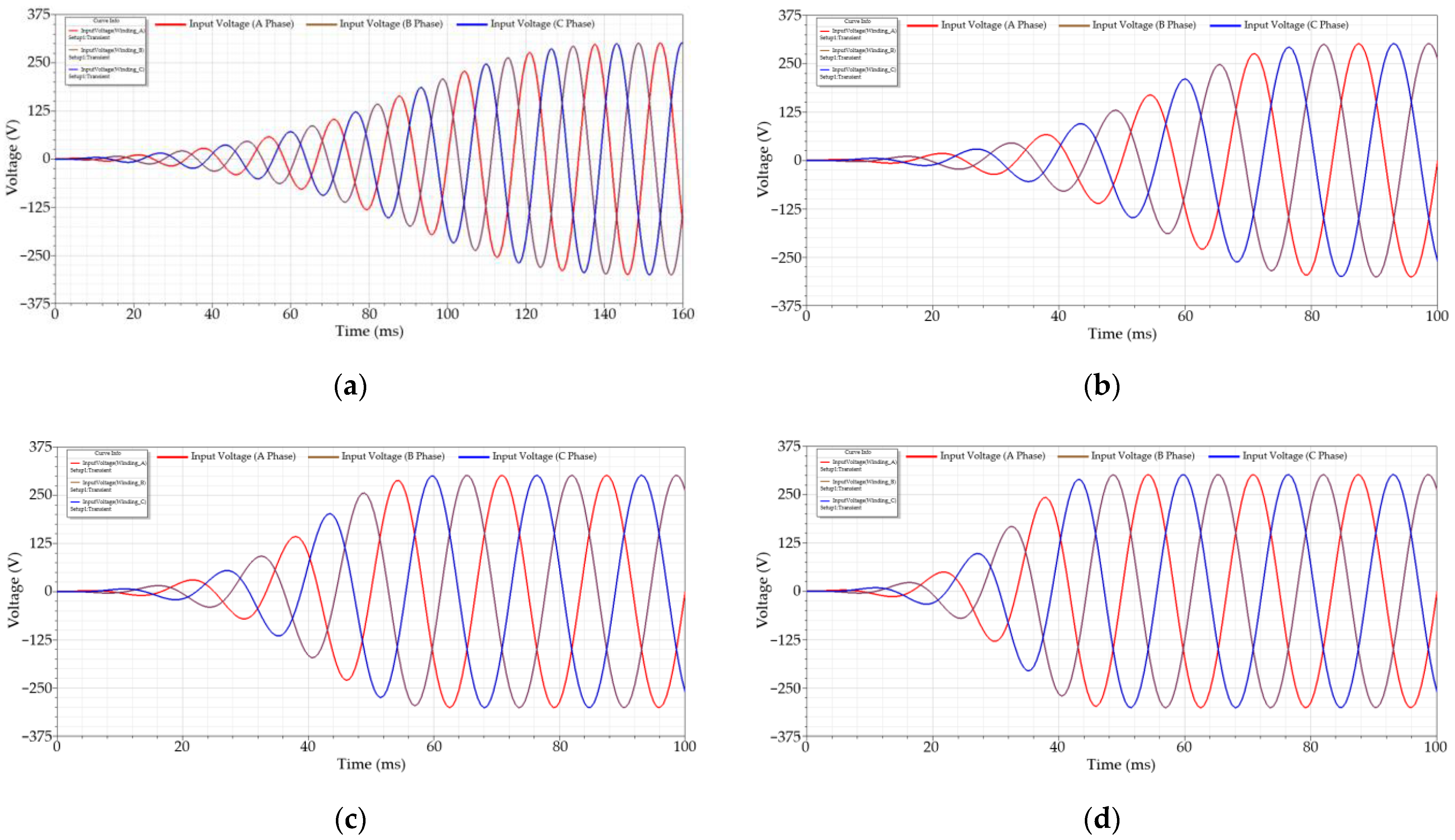
Figure 8.
Simulation results of the winding flux linkage without a slow start.
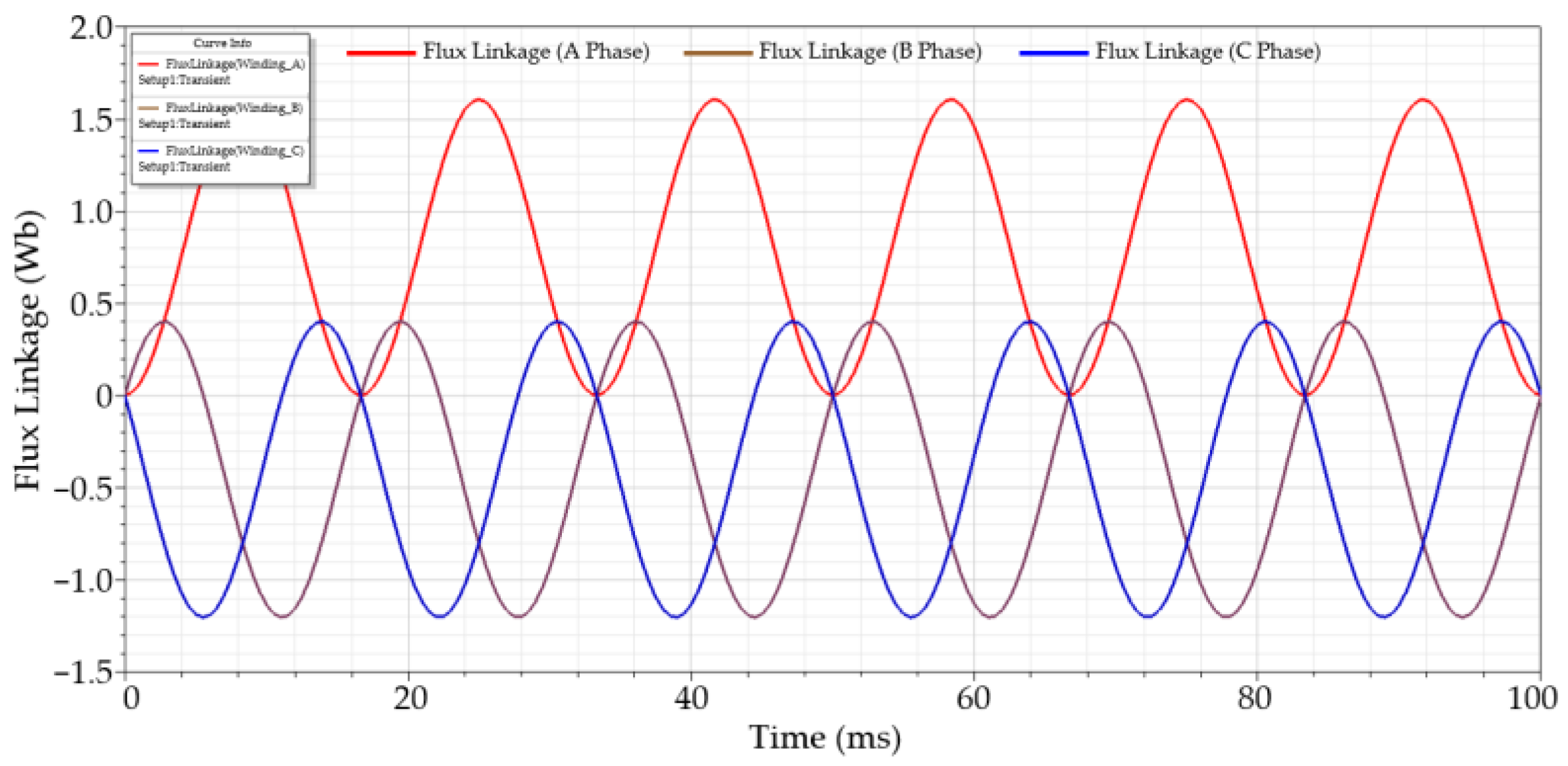
Figure 9.
Simulation results of the winding flux linkage under the conventional equation. (a) ; (b) .
Figure 9.
Simulation results of the winding flux linkage under the conventional equation. (a) ; (b) .
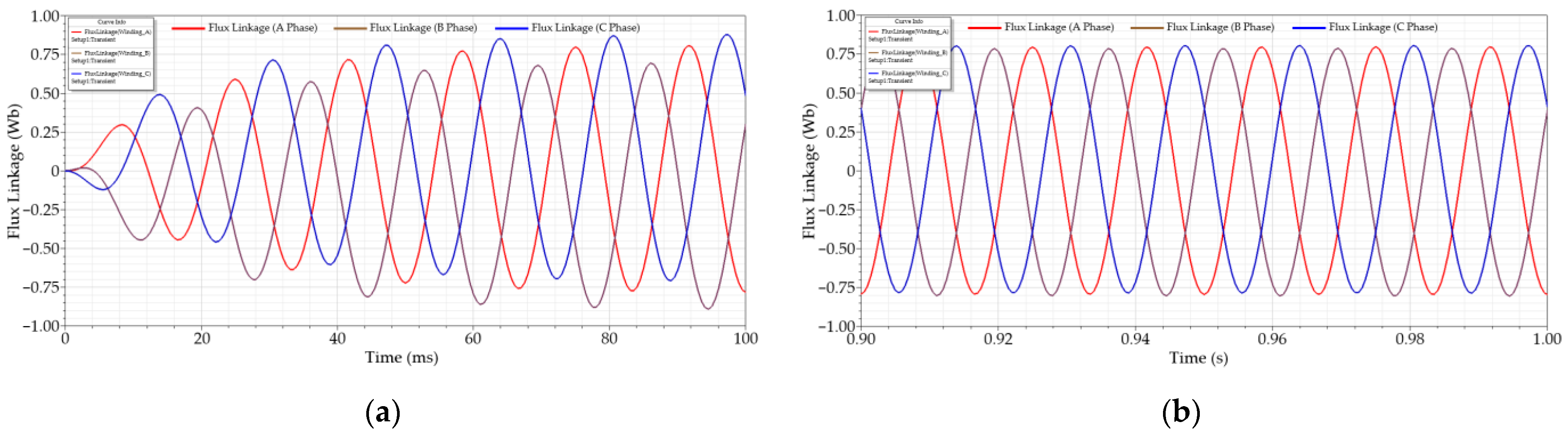
Figure 10.
Simulation results of the winding flux linkage under the proposed equation. (a) ; (b) ; (c) ; (d) .
Figure 10.
Simulation results of the winding flux linkage under the proposed equation. (a) ; (b) ; (c) ; (d) .
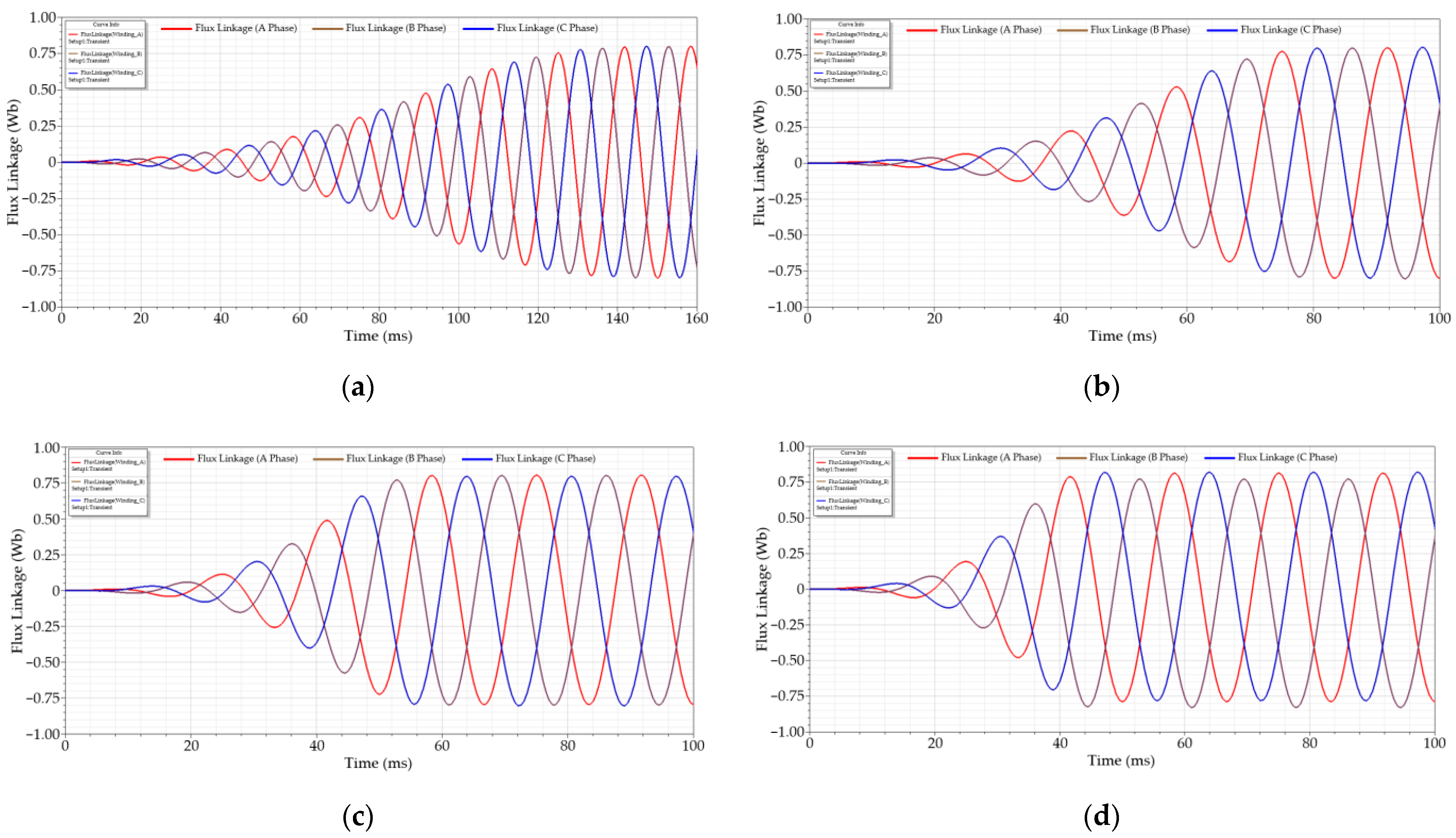
Figure 11.
Simulation results of the core loss without a slow start.

Figure 12.
Simulation results of the core loss under the conventional equation. (a) ; (b) .

Figure 13.
Simulation results of the core loss under the proposed equation. (a) ; (b) ; (c) ; (d) .
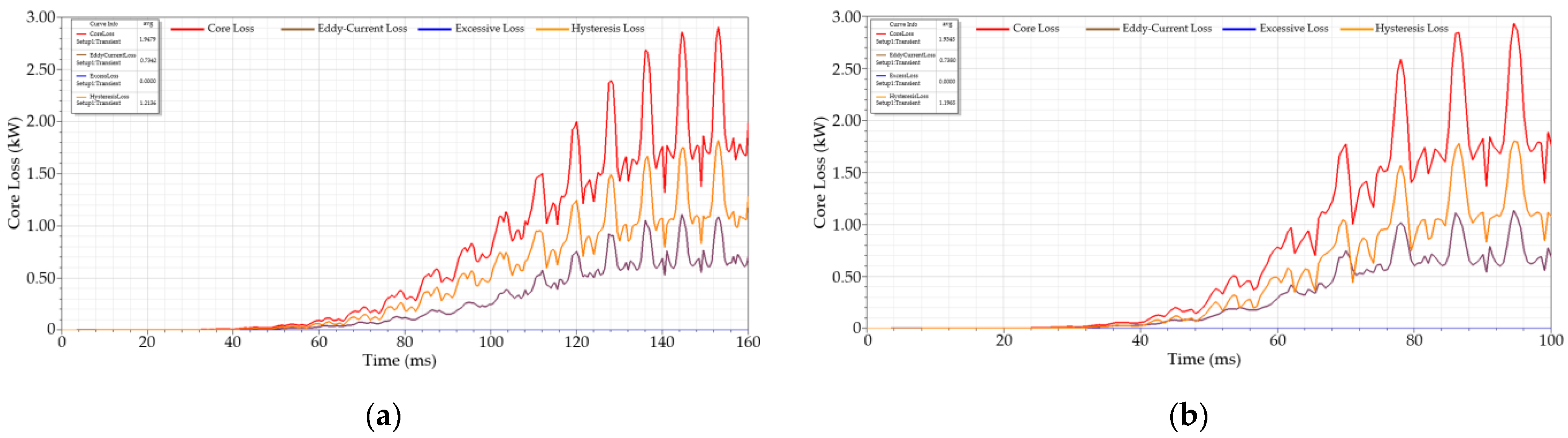
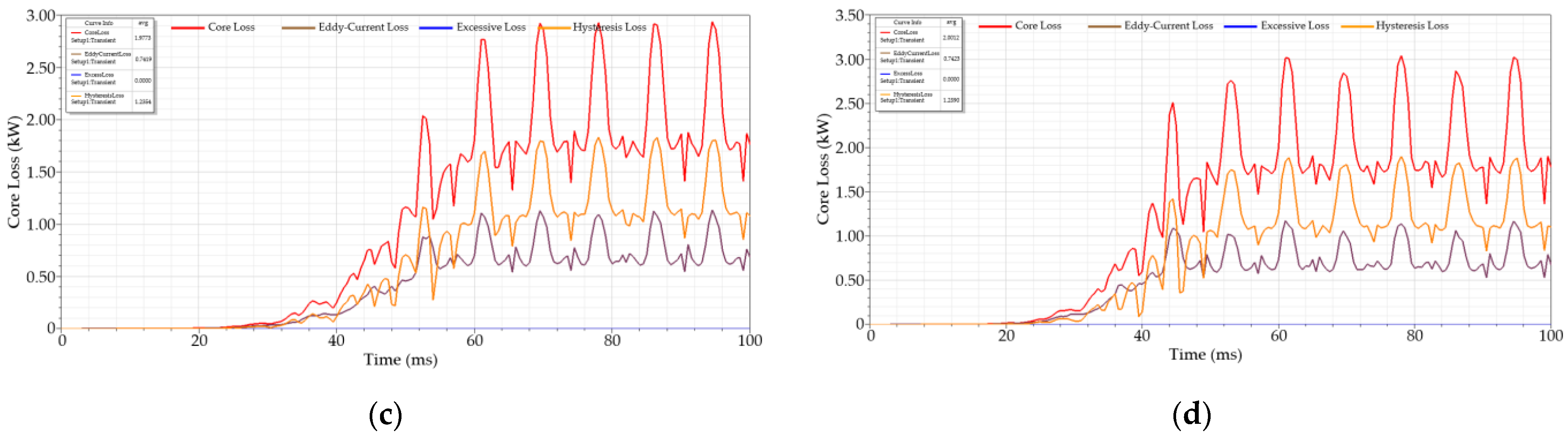
Figure 14.
The simulation results of the magnetic flux density distribution under different external excitation functions.
Figure 14.
The simulation results of the magnetic flux density distribution under different external excitation functions.
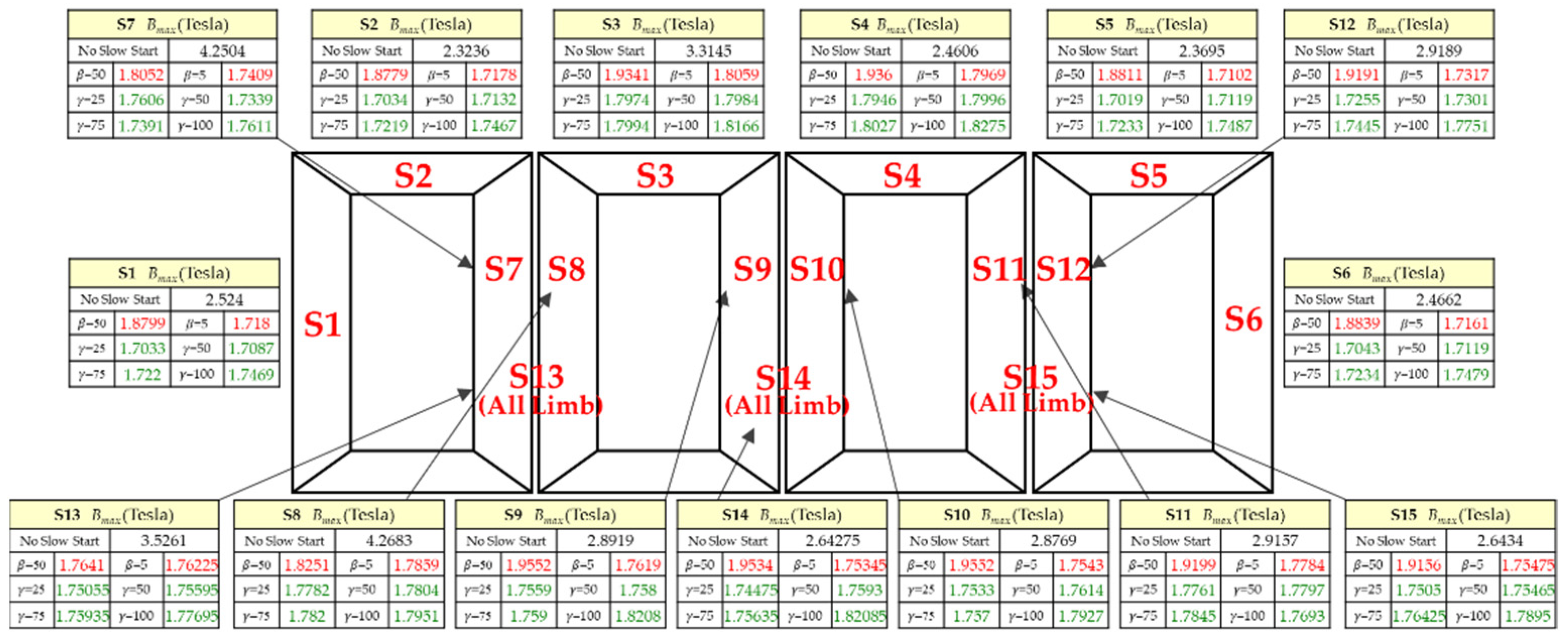
Figure 15.
Setting diagram of the three-phase five-limb transformer.

Figure 16.
The measured three-phase five-limb transformer diagram.

Table 1.
The parameters of the simulation model.
| Name | Parameter |
|---|---|
| Length of Single Limb | 480 mm |
| Depth of 2D Model | 10.3354 mm |
Table 2.
Materials of the simulation model.
| Name | Material | Parameter |
|---|---|---|
| Excitation Coil | Copper | Resistivity: 1.68 × 10⁻⁸ [Ω m] |
| Iron Core | Electrical Grade Sheet | Conductivity: 2,083,300 [S/m] Mass Density: 7650 [kg/m3] Relative Permeability: Non-linear B-H Curve |
| Gap, Environment | Air | Magnetic of Relative Permeability: 1.0000004 |
Table 3.
Loss coefficients of the iron core (@60 Hz).
| Name | Parameter |
|---|---|
| Coefficient of Hysteresis Loss kh | 0.00581484 W/kg |
| Coefficient of Eddy Current Loss kc | 3.26563 × 10⁻⁵ W/kg |
| Coefficient of Excessive Loss ke | 0 W/kg |
Table 4.
Parameters of external excitation.
| Name | Parameter |
|---|---|
| Peak Voltage (Vpeak) | 301.64 V |
| Frequency () | 60 Hz |
| Slow Start Parameters of Conventional Equation | 5, 50 |
| Slow Start Parameters of Proposed Equation | 25, 50, 75, 100 |
Table 5.
Simulation results of the core loss under different slow start functions.
| Name | Core Loss | Hysteresis Loss | Eddy Current Loss |
|---|---|---|---|
| No Slow Start Condition | 2.4093 kW | 76.92% | 23.08% |
| Convention Equation () | 2.0087 kW | 64.43% | 35.57% |
| Convention Equation () | 1.9563 kW | 62.75% | 37.25% |
| Proposed Equation () | 1.9479 kW | 62.30% | 37.70% |
| Proposed Equation () | 1.9345 kW | 61.85% | 38.15% |
| Proposed Equation () | 1.9773 kW | 62.48% | 37.52% |
| Proposed Equation () | 2.0012 kW | 62.91% | 37.09% |
Table 6.
Experimental results of magnetic flux density under different test coils.
| Name | Measured Value | Simulation Results Error | ||||||
|---|---|---|---|---|---|---|---|---|
| No Slow Start | ||||||||
| S1 | 1.5782 T | 59.92% | 19.11% | 8.47% | 7.92% | 8.26% | 9.11% | 10.68% |
| S2 | 1.5843 T | 46.66% | 18.53% | 8.05% | 7.51% | 8.13% | 8.68% | 10.25% |
| S3 | 1.7072 T | 94.14% | 13.29% | 4.71% | 5.28% | 5.34% | 5.40% | 6.40% |
| S4 | 1.6983 T | 44.88% | 13.99% | 6.08% | 5.67% | 5.96% | 6.14% | 7.60% |
| S5 | 1.5571 T | 52.17% | 20.80% | 10.02% | 9.29% | 9.94% | 10.67% | 12.30% |
| S6 | 1.5263 T | 61.58% | 23.42% | 12.24% | 11.66% | 12.16% | 12.91% | 14.51% |
| S7 | 1.6167 T | 162.90% | 11.65% | 6.21% | 8.90% | 7.24% | 7.57% | 8.93% |
| S8 | 1.7058 T | 150.22% | 6.99% | 3.80% | 4.24% | 4.37% | 4.46% | 5.23% |
| S9 | 1.6957 T | 70.54% | 15.30% | 3.90% | 3.55% | 3.67% | 3.73% | 7.37% |
| S10 | 1.7088 T | 68.35% | 14.41% | 3.34% | 2.60% | 3.07% | 2.82% | 4.90% |
| S11 | 1.6746 T | 74.11% | 14.64% | 6.39% | 6.06% | 6.27% | 6.56% | 5.65% |
| S12 | 1.5928 T | 83.25% | 20.48% | 8.87% | 8.33% | 8.62% | 9.52% | 11.44% |
| S13 | 1.6756 T | 110.43% | 5.28% | 4.00% | 4.47% | 4.79% | 4.99% | 6.04% |
| S14 | 1.6884 T | 56.52% | 15.69% | 4.45% | 3.33% | 4.19% | 4.02% | 7.84% |
| S15 | 1.6595 T | 59.28% | 15.43% | 5.91% | 5.48% | 5.73% | 6.31% | 7.83% |
Table 7.
Experimental results of the core loss.
| Name | Core Loss | Error |
|---|---|---|
| Measured Value | 1.949 kW | 0% |
| Simulation Results (No Slow Start) | 2.4093 kW | 23.61% |
| Simulation Results (Conventional Equation, ) | 1.9545 kW | 0.28% |
| Simulation Results (Conventional Equation, ) | 2.0684 kW | 6.12% |
| Simulation Results (Proposed Equation, = 25) | 1.9479 kW | 0.056% |
| Simulation Results (Proposed Equation, = 50) | 1.9345 kW | 0.743% |
| Simulation Results (Proposed Equation, = 75) | 1.9773 kW | 1.452% |
| Simulation Results (Proposed Equation, = 100) | 2.0012 kW | 2.678% |
Publisher’s Note: MDPI stays neutral with regard to jurisdictional claims in published maps and institutional affiliations. |
© 2021 by the authors. Licensee MDPI, Basel, Switzerland. This article is an open access article distributed under the terms and conditions of the Creative Commons Attribution (CC BY) license (https://creativecommons.org/licenses/by/4.0/).
Share and Cite
MDPI and ACS Style
Chang, W.-C.; Kuo, C.-C. A Novel Excitation Approach for Power Transformer Simulation Based on Finite Element Analysis. Appl. Sci. 2021, 11, 10334. https://doi.org/10.3390/app112110334
AMA Style
Chang W-C, Kuo C-C. A Novel Excitation Approach for Power Transformer Simulation Based on Finite Element Analysis. Applied Sciences. 2021; 11(21):10334. https://doi.org/10.3390/app112110334
Chicago/Turabian StyleChang, Wen-Ching, and Cheng-Chien Kuo. 2021. "A Novel Excitation Approach for Power Transformer Simulation Based on Finite Element Analysis" Applied Sciences 11, no. 21: 10334. https://doi.org/10.3390/app112110334
Note that from the first issue of 2016, this journal uses article numbers instead of page numbers. See further details here.