
Experimentally Viable Techniques for Accessing Coexisting Attractors Correlated with Lyapunov Exponents


Department of Physics, Oklahoma State University, Stillwater, OK 74078, USA
*
Author to whom correspondence should be addressed.
Appl. Sci. 2021, 11(21), 9905; https://doi.org/10.3390/app11219905
Submission received: 1 September 2021
/
Revised: 18 October 2021
/
Accepted: 20 October 2021
/
Published: 23 October 2021
(This article belongs to the Special Issue Quantum Dot Lasers and Laser Dynamics)
Abstract
:Universal, predictive attractor patterns configured by Lyapunov exponents (LEs) as a function of the control parameter are shown to characterize periodic windows in chaos just as in attractors, using a coherent model of the laser with injected signal. One such predictive pattern, the symmetric-like bubble, foretells of an imminent bifurcation. With a slight decrease in the gain parameter, we find the symmetric-like bubble changes to a curved trajectory of two equal LEs in one attractor, while an increase in the gain reverses this process in another attractor. We generalize the power-shift method for accessing coexisting attractors or periodic windows by augmenting the technique with an interim parameter shift that optimizes attractor retrieval. We choose the gain as our parameter to interim shift. When interim gain-shift results are compared with LE patterns for a specific gain, we find critical points on the LE spectra where the attractor is unlikely to survive the gain shift. Noise and lag effects obscure the power shift minimally for large domain attractors. Small domain attractors are less accessible. The power-shift method in conjunction with the interim parameter shift is attractive because it can be experimentally applied without significant or long-lasting modifications to the experimental system.
1. Introduction
The influential research in optical bistability (OB) by Bonifacio and Lugiato [1,2] undergirds the many investigations of the active counterpart of OB, the laser with injected signal (LIS). The LIS system is well-studied and covers a broad range of active systems, including CO2, diode [3,4,5], and quantum dot lasers [6,7]. It is replete with interesting dynamics from chaos to coexisting attractors [8,9,10]. Intriguing glimpses into self-similarity are reported in References [11,12,13]. Some, if not all, of these characteristics can be found in a wide variety of other models and nonlinear systems [14,15,16,17].
Nonlinear dissipative systems have challenged the imagination since the late 1970s with their potential, unique dynamic features and chaotic behavior [18,19,20,21,22]. The discovery of multistability energized innovative approaches such as feedback loops. Experimentally, Gibbs et al. [23] found that delayed feedback could induce multiple coexisting attractors in an electro-optical bistable device. Coexisting attractors with subharmonic output frequencies were experimentally observed in a modulated CO2 laser by Arecchi et al. [24]. Later, bifurcation diagrams of a modulated CO2 laser assisted the experiment; these diagrams were made by sweeping one of the control parameters in an attempt to find bistability [25,26,27,28]. However, the continuous changes of the control parameter limited which attractors could be isolated because of hysteresis effects. Theoretical contributions by Meucci et al. [29] used stepwise changes in a modulated frequency to cause switching between two coexisting attractors in a multistable system.
System control was studied further by Ott, Grebogi, and Yorke [30] and Pyragas [31] who set about controlling chaos using feedback methods that did not require, a priori, analytical knowledge of the system dynamics. The approach was limited because the feedback loop altered the state variables or system parameters. In 2014, Li and Sprott used amplitude control to detect multistability and coexisting attractors [32]. Later, an offset-boosting-based approach was developed as well for the identification of multistable dynamical systems [33]. Burton et al. [34] developed a power-shift method that changed only the control parameter of the system to transition from one attractor to another. However, the method requires some trial and error. A way to avoid this process may exist in the traditional theoretical tools, for example, the analysis of Lyapunov exponents (LEs), which is discussed further in Section 4.2.1.
Lyapunov exponents are able to identify spectral patterns of Hopf bifurcations, period-doubling episodes, tori, and chaos [10,35]. In 2015 Bandy et al. [36] reported that globally analyzed Lyapunov exponents could be used to identify attractor coexistence by comparing forward and backward global scans of the LEs. Lyapunov spectra also predicted the trends of the fundamental frequencies of the output signal of the individual attractors. Structural patterns in the Lyapunov spectra were observed, but the pattern formation was not correlated with the dynamic behavior of the attractor. Later, these specific LE patterns were discovered to predict bifurcation sequences, imminent bifurcations, and common borders of the attractor domains [37]. An imminent bifurcation predicts that by slightly changing a system parameter, one LE pattern changes into another signifying a bifurcation in the system.
Herein, we report further findings of pattern formations that predict imminent potential changes in the dynamics provided the gain parameter is modified slightly. We identify the correlation between these LE configurations and the different values of the gain parameter. Specifically, we see an attractor with a curved trajectory of two equal LEs that appears to be benign with respect to its dynamic behavior. A slight increase in the gain produces a symmetric-like bubble whose potential dynamic characteristic is an established pattern identified in Reference [37]. Also, by slightly decreasing the gain of the system, a symmetric-like bubble known to exist in another attractor changes to the curved trajectory of two-equal LEs, just the reverse of the previous attractor event. Because these two cases represent two different attractors with two different modifications to the gain, what appears to be obvious now, are in fact, new universal pattern constructs with identifiable dynamic connections, albeit future system dynamics.
We also report findings that describe a method for discovering the ideal base attractor used in power shifting the LIS system. We examine the location of the ideal shift and explore correlations with the apexes of the LE bubbles in an attractor’s LE spectra. The experimental conditions of the power shift are developed by including noise on the frequency of the injected signal and a linear ramp on the amplitude of the injected signal. Finally, we create a generic counterpart to the power shift, called the interim parameter shift, in which a system parameter is temporarily modulated to transition to attractors, i.e., to systematically access coexisting attractors and windows in chaos. The interim parameter shift results are compared with the LEs to check for correlations between the reliability and the stability of the system.
2. Model and Methods
2.1. Laser with Injected Signal Model
The laser with injected signal is a semi-classical theory that is based on a homogeneously broadened 2-level atom. The atoms and the cavity frequencies, ωa and ωc, respectively, are tuned usually to one another at ωa = ωc and, in the absence of the external signal, produce a stable laser output with a carrier frequency ωa. By injecting into the cavity a continuous wave beam at frequency ω0 ≠ ωa, the potential for competition is established between the driving field and the laser oscillator. At resonance and low input-signal levels, beat patterns with frequencies close to |ωa − ω0| appear because of a simple mixing of the 2 fields, and thus, the laser acts as the local oscillator. At a high external signal amplitude, the laser is predicted to stably lock to the injected field and produce a constant output intensity, known as injection locking with a carrier frequency ω0. Between these 2 limits, complicated and interesting nonlinear phenomena appear and, contingent on the system parameters, there are still many unexplained dynamic events. For example, the output signal can display coexisting incommensurate frequencies [35] or as many as 3 different commensurate frequencies for the same driving field by using slightly different initial conditions [8,10,36].
The laser with injected signal is based on the Maxwell-Bloch equations and defined by the customary single-mode, non-resonant unidirectional ring laser. It is a coherent model designed to approach most closely the conditions of spatial uniformity; the chosen parameters are intermediate to the conditions of Class B [38] and Class C [39] lasers. The representative nonlinear equations are as follows:
where Y is real and positive for definiteness (the system control parameter) and is proportional to the incident field amplitude; X and P are the complex field and polarization amplitudes; D is the real population difference, where negative numbers represent the excited states. We chose to study the equations as 5 real differential equations. The system parameters are the small-signal atomic gain C, the scaled cavity relaxation rate = κ/γ⊥, the scaled population decay rate = γ∥/γ⊥, the scaled cavity mistuning parameter Φ = (ω0 − ωc)/γ⊥, and the scaled atomic detuning from the injected-signal carrier = (ωa – ω0)/γ⊥. γ∥ is the relaxation rate of the population inversion and γ⊥ is the polarization relaxation rate. The time τ is measured in units of the polarization relaxation time γ⊥−1. The system parameters are C = 3, = 0.5, = 0.1, = 0.01, Φ/ = −0.5. If Equations (1) and (2) are written in terms of their real and imaginary components, then these equations can be written as real first-order differential equations; adding the real population difference makes a total of 5 real equations which we use to study the nonlinear LIS system. The numerical routine used to solve these equations was the NDSolve function in Mathematica, using the “StiffnessSwitching” method.
In steady state, the output field amplitudes are triple valued with respect to the injected signal, with a domain of instability of 0 < Y < 2.17; the entire lower branch of the tripled-value-curve is unstable.
2.2. Lyapunov Exponents
Lyapunov exponents are theoretical spectra used to study nonlinear dynamics and mathematical maps. They describe the average growth or decay of infinitesimal perturbations to an n-dimensional system orbit and are invariant with respect to their pattern formations and respective domains. In physics, there is universal agreement that even one positive LE predicts chaotic dynamics or fractal geometry [40,41,42]. In this study, the largest three LEs of the 5 available are the dominant contributors to the universal attractor pattern formations described by Bandy et al. [37]. The 2 lowest LEs are not represented here; however for completeness, we note that they are more negative than the others and are always equal for this set of parameters, see Figure 13b and Figure 16b in Reference [36]. The LE order may be different for pattern formation in other nonlinear systems, but the same universal attractor patterns are evident. By attractor pattern formation we mean a universally defined visual arrangement of the LEs as a function of the control parameter. We calculate LEs from a modified form of the Benettin method [43] as applied in the Appendix of Reference [35].
Attractor domains are calculated as an adiabatic scan of the injected signal, so that once located on the attractor, small steps of the control parameter can be taken successively to hold the system on the attractor until it no longer exists. See Reference [36] for details. The scan step size provides the precision for the LE spectral features within the attractor domain. In this study, the details of the system dynamics being explored provide the guidelines for the injected-signal step size. Fourier transforms, Poincarè maps, phase-space portraits, bifurcation diagrams, and temporal plots are the supporting theoretical tools used to confirm the dynamics predicted by the various LE patterns.
Probing nonlinear behavior and multistability, whether in a physical model or a map, is a system-dependent exercise. We chose a single mode, coherent model of the laser with injected signal because it is a generic archetype of the aforesaid LIS model and because there are extensive experimental studies of similar systems. For example, multistability was observed in 1982 by Arecchi et al. [24] using a loss-modulated CO2 laser; they experimentally established proof-of-existence of coexisting attractors, sparking a new era of LIS research. The LIS studies herein were influenced profoundly by their results. Research varies from exploring system nonlinearities [8,10] to examining intertwined studies of nonlinearities and coexisting attractors [35,36]. In 1985, investigations [35] unearthed many strange looking global LE patterns which, at the time, were considered mysterious if not bizarre spectra. By 2015, these strange looking LE formations (patterns) were no longer considered random prattle. They were found to be significant universal configurations that predicted the dynamic behavior of LIS and other nonlinear systems. The LE formations are known to predict: (i) the domains of coexisting attractors (see Figure 13 of Reference [36]), (ii) a universal attractor boundary, and (iii) characteristic dynamic behaviors (both current and imminent) that are best understood in the context of 2-parameter (“shrimp”) diagrams in Reference [13].
Figure 1 represents a schematic of attractor and window domains for the parameters under consideration. Attractor and window dynamics are included as a function of the injected signal. Each attractor is graphed by the position of its relative characteristic frequency and its domain of activity. The information summarized in Figure 1 is calculated using both LEs and traditional theoretical tools as stated above. Each attractor and window domain is identified by name; attractor 1 (AI) to attractor 8 (AVIII) and periodic windows WI and WII, and their dynamic features. They are named in the order in which they were discovered. Figure 1 is especially useful when one tries to understand the relative positioning of the coexisting attractors; it is also an instant visual of their general dynamics. AI and AII have special distinction from the other attractors in that they appear to be the scaffolding upon which other attractors coexist, except for AVII and AVIII which coexist with chaos. WI and WII interrupt chaos. AI brings LIS to life for low values of the injected signal, while AII has the largest attractor domain and guides the system into injection locking. Note, that some Y values label period-doubling episodes: for example, in AI and AII there is a 2n period-doubling sequence and in AVII a 5 × 2n doubling sequence. The transition from 6P to 12P identified in AIV refers to the two dominant limit cycles of a period-doubling sequence, 6 × 2n into chaos. The callouts for AI, AIV, AII, AVII, and AVIII magnify some details of the attractor dynamics. For example, inverse bifurcation sequences are identified in the callouts AII and AVII.
Different theoretical tools provide information about an attractor or window dynamics and that includes chaos, but it is the exploration of the LEs as a function of the system’s control parameter that reveals the detailed, universally predictive information about each attractor [37] or window. In addition, the study of LE patterns leads ultimately to understanding how an attractor can be accessed reliably under experimental conditions without changing the parameters of the system itself. It is called a power shift [34].
2.2.1. Generic Attractor Characteristics
To date, we have identified the following generic attractor characteristics that are predicted by LEs. A common attractor LE spectral boundary outlines the borders of each of the attractor and window domains. A 2-zero LEs’ signature that is common to several other spectral patterns indicates the beginning and ending of each attractor’s existence [37]. That is, as the injected signal is either increased or decreased, the point of the attractor’s origin or demise is a pair of zero LEs. In between these two extremes, the attractor’s spectral pattern evolves as the dynamics dictate. Figure 2a displays each attractor via its LE pattern in the context of the total unstable LIS domain for this set of parameters. In Figure 2b–d individual LE attractor domains are displayed corresponding to A, B, and C in Figure 2a. Each exhibits the characteristic boundary of converging and diverging Lyapunov spectra and the signature zero pair of LEs. The 8 known attractors are color coded as follows: AI is burnt orange, AII is red, AIII is green, AIV is purple, AV is blue, AVI is yellow, AVII is gray, and AVIII is pink.
A cluster of asymmetric LE bubbles along with their signature zero-pair LEs’ at their apexes represent a forward (in AVII and AVIII) or backward bifurcation sequence, (in AIV); how the sequencing evolves can be interesting. See results in Section 3.1. Figure 2a displays one symmetric bubble in AIII, but this characteristic pattern indicates a different type of dynamics other than the asymmetric bubbles. The following discussion elaborates on symmetric-like LE bubbles.
2.2.2. Symmetric-like LE Bubbles
The symmetric-like bubble emerges as a Lyapunov spectral pattern that predicts imminent changes in the dynamics when a parameter is modified slightly. The bubble has an apex located near its center that is not a zero LE. We suspect this apex has something to do with the probability of transitioning dynamics when one of the parameters of the system is changed. There is more discussion on this in Section 4.3. The function of the symmetric-like bubble becomes clearer when linked to the studies of Bonatto et al. [12,13] and Mandel and Erneux [44]. The symmetric-like bubble is now understood to be the forerunner to an imminent bifurcation in the system dynamics, when one of the parameters, such as the gain, is changed. To examine the effects of changing the gain on the attractor dynamics, we collect the LEs associated with “corkscrew” attractors: AIII, AV, and AVI and discuss further in Section 3.1.
2.2.3. Window Characteristics Predicted by Lyapunov Exponents
In Figure 3 we present 2 unique LE profiles of windows in chaos, WI and WII, that are graphed within their domains as a function of Y. The 2-color scheme in each graph of WI and WII is the result of forward (black) and backward (red) scans of their domains. Note, that the backward scan is not an exact replica of the forward scan. Since these scans are executed adiabatically, the accuracy of landing on WI or WII is imperfect. That is, we believe, the backward scan follows the chaotic trajectories temporarily because the accuracy of the calculations is insufficient to acquire WI and WII at their demise.
It is easy to see that as a function of the control parameter Y, the 2 windows of Figure 3 possess asymmetric bubble patterns. The significance of these results is that windows can be identified using LEs in the same way that attractors are identified. Further, the discovery of the windows in this study was made using the power-shift method [34], as described in Appendix A. By dividing the range ΔY into 1001 segments and evolving for T = 20,000τ at Y = 1.229 we found WI and at Y = 1.2575 we found WII.
2.3. Power Shifting to Access Attractors or Windows
2.3.1. A Theoretical Example of Power Shifting
The power-shift (PS) method requires a nonlinear system with an independent control parameter. Power shifting is a type of incremental perturbation of the control parameter with the result of either accessing known or discovering new attractors (or windows). The method employs specific timings to steer the dynamic trajectory from one known attractor to another that may even coexist.
The power-shift method works in the laser with injected signal by changing the input signal Y at specific points on a known stable limit cycle. In Figure 4a there are 2 sets of limit cycles of known attractors superimposed on each other. The magenta x on base AVI (period four limit cycle in green) marks the position where the injected signal is down shifted from Y0 = 1.96 to YPS = 1.84. The system trajectory jumps from base AVI to resultant AV (period three limit cycle in blue). In Figure 4b for a different location on base AVI, again marked by a magenta x, we show that the system trajectory moves off base AVI to resultant AII using the same down shift values from Y0 = 1.96 to YPS = 1.84. Note, AV and AII coexist at Y = 1.84.
2.3.2. Power-Shift Base Attractor Optimization
In this investigation we use the power-shift method to collect the statistics associated with the successful access of a desired attractor. We initialize the system on the base attractor for 1 control parameter value Y0 and power shift to YPS while at different locations on the limit cycle uniformly distributed in time. For convenience, we set 1 point on the limit cycle as the reference point. An obvious choice for the reference point is the time associated with the attractor’s peak-output power. Next, select any location on the limit cycle as the time after the peak (TAP). We observe to which attractor each TAP evolves. Finally, select a new Y0 usually in increments of ΔY0 = 0.01 and repeat the investigation for the same power shift, YPS. The results are tabulated across the domain of the base attractor and evaluated for the largest tranche (or time intervals) of TAPs that accesses the desired attractor, or it might be said, for the most efficient Y0 of the base attractor domain.
An experimentalist might choose to time the power shift at the middle of the tranche, because it gives the largest allowable margin of error for a successful power shift. In the following discussion we include noise and ramp the injected signal.
2.3.3. Power Shift with Noise and Ramped Injected Signal
The power-shift method can be altered theoretically by applying noise to the injected signal frequency at regular intervals in time with an amplitude range simulating experimental conditions more accurately. We add noise with amplitude 0.015 to the injected signal frequency every 0.4τ using the RandomReal function in Mathematica. The addition of noise in the injected signal frequency does modify slightly the system parameters and Φ to comport with the model. The change is insignificant.
The second modification of the power-shift method’s experiment is to apply a linear ramp to the power-shift amplitude instead of the Heaviside function initially used. In experiment, an actual laser does not instantaneously reach its new power. To simulate the lag effect, we select power shifts of the type Y(τ,TAP) = Y0 + slope(τ-TAP), slope = (YPS − Y0)/Tlag. See Section 3.2.1 for the results of the data collection.
2.3.4. Interim Parameter (Gain) Shift
The interim parameter (gain-)shift functions in the following way: Start on a limit cycle and abruptly change the value of the gain for a certain amount of time and then shift it back to its original value. This may result in accessing a different attractor. For our study, we select the gain parameter, because it is convenient and works well as an experimental adjustable. To interim gain shift, we begin at the peak electric field output as the initial condition at t = 0 and allow the system to evolve along the limit cycle until we reach the desired TAP. At that point, we slightly change the gain from its original value to its new value. After an arbitrary t = 10,000τ we shift the gain back to its original value and record the trajectory’s evolution to the resultant attractor. For this study we chose to shift through AIII’s domain; we record different TAP tranches on the limit cycle and determine the statistical distribution resulting from the gain shift. This gives the percentage chance the system leaves its original (base) attractor. See Section 3.3 for results.
3. Results
3.1. Gain Changes on Lyapunov Exponent Patterns
In Figure 5a–c we calculate the LEs of AIII using different gains (C values), one value lower than C = 3.0 and the other value larger. The LE pattern, Figure 5a, at a lower value of C = 2.7 no longer exhibits a symmetric-like bubble; it is replaced by a curved trajectory of two equal LEs. A change to a higher value of C = 3.1 shows the LE replacement as the expected asymmetric bubble in Figure 5c, described in Reference [37]. The LE patterns of AIII at C = 2.7 resemble the LE patterns of AV and AVI at the standard (canonical) C = 3.0. Because of their resemblance, we then explored the LEs for AV and AVI to inspect their evolutionary LE pattern changes when C increases from 3.0, to 3.1 and 3.2 for AV, and C increases from 3.0, to 3.2, 3.25, 3.3, and 3.35 for AVI. The results are shown in Figure 5d–f and Figure 6, respectively.
3.2. Power Shift
3.2.1. Optimized Base Attractor for Power Shift
We demonstrate optimized power–shift conditions for a base attractor in Figure 7. Figure 7a plots the largest tranches (time intervals) that transition to AV as a function of Y in AIII’s domain when power shifted to YPS = 1.84; the domain is divided into steps of ΔY0 = 0.01. We find the power shift at Yo=1.63 has the largest tranche for transitioning to the desired AV. Figure 7b uses the same conditions as Figure 7a except the power shift changes to YPS = 1.96 to access the desired AVI. This optimization scheme can be achieved for any valid set of base and goal attractors.
Figure 8a shows results beginning on base AIII at Y0 = 1.63 and power shifted to YPS = 1.84 every 1τ along the period of motion. The resultant attractors, AV or AII, are recorded. The blue and red segments illustrate along the temporal period, 163.551τ, the system’s viable tranches where either AV or AII can be found, respectively. In Figure 8b we show the results beginning on base AIII at Y0 = 1.72 and power shifted to YPS = 1.96 for every 1τ. The resultant attractors, AVI or AII, are recorded. Note, at the end of one period is the beginning of the other, so we can combine the points on both ends to configure the total tranche size. In this case we had 101 contiguous points in a single period of AIII going to the desired AV in Figure 8a and 55 contiguous points going to the desired AVI in Figure 8b.
3.2.2. Addition of Noise
3.2.3. Linear Ramp on Injected Signal
In Figure 10 we modify the power-shift method with a time lag, Tlag = 15, at Y0 = 1.63 for base AIII with the YPS = 1.84 to simulate experimental conditions. Graphing two periods of the motion dramatizes the range of the tranche that goes to AV using a linear ramp.
3.2.4. Linear Ramp and Noise Included
3.3. Interim Gain-Shift Results
Figure 12 illustrates the results of an interim gain shift lasting for 10,000τ by plotting the percent chance AIII survives the shift from C = 3.0 to C = 3.1 as a function of Y. Clearly for this shift, there is a high percentage of AIII surviving with some intermittencies when Y ≥ 1.64. No experimental complications are addressed in this study.
4. Discussion
4.1. Gain Change Effects on LE Patterns
Gain parameter changes clearly affect LE patterns because they alter the parameters of the system. As discussed in Section 3.1 and shown in Figure 5a, the gain is decreased from the canonical C = 3.0 to C = 2.7; here the symmetric-like bubble is eliminated leaving a pattern similarly matching the canonical AV and AVI. In Figure 5b,c the gain is increased from C = 3.0 to C = 3.1, respectively. Due to this slight increase, a symmetric-like bubble changes to an asymmetric bubble supporting the hypothesis that symmetric-like bubbles represent an imminent bifurcation in the system. In Figure 5d–f the gain parameter increases from the canonical C = 3.0 to C = 3.2, where there is a first transition to a symmetric-like bubble, and second to an asymmetric bubble, confirming the thesis that symmetric-like bubbles are predictors of an imminent bifurcation provided there is a small change to one parameter of the system. Note, this result is consistent with the studies in References [13,44] who confirm these types of dynamic changes. It is interesting that a new symmetric-like bubble emerges in Figure 6d forecasting the bifurcation shown in Figure 6e.
4.2. Power Shift
4.2.1. Optimized Power Shift
We find AIII has the largest tranche of points that transition to AV at Y0 = 1.63 when power shifted to YPS = 1.84. For accessing AVI, we find AIII’s largest tranche is at Y0 = 1.72 when power shifted to YPS = 1.96. The largest tranche going to AVI is close to the peak of the symmetric-like LE bubble in AIII. The results for accessing AVI, however, also support the theory because the largest tranche is located only ΔY = 0.005 from the apex. The results for AV, however, do not support the hypothesis that the apex of the symmetric-like bubble is the ideal value from which to power shift, because the largest tranche exists at a much lower value of Y.
The location of the largest tranches for each attractor can be tabulated theoretically to create a “roadmap” of the system describing the most effective way to access every attractor solely through power shifting. See Appendix B, Table A1, as an example.
4.2.2. Effects of Noise
As expected, noise induces some changes indicated by the intermittent transitions to AII in Figure 9, where the tranche of AV dominates without noise, as shown in Figure 8a. At this level of noise, we can say that the power-shift method is still viable. However, because of the intermittencies to AII, it may take multiple tries to access the desired attractor. Note, AIV, AVII, and AVIII are all small domain attractors which are difficult generally to access. Preliminary tests show noise will most likely prevent any access to these three attractors. Clearly AIII, AV, and AVI have larger domains and survive small amounts of noise. AIII, which has the largest domain of AV and AVI, survives a greater noise amplitude.
4.2.3. Effects of a Ramp on the Injected Signal
We compare the power-shift method with and without the linear ramp on the control parameter. In Figure 13 we show the resulting attractor vs. TAP. The blue dots represent the stepwise injected signal at Y0 = 1.63 for base AIII with the YPS = 1.84, i.e., with no Tlag. The orange xs represent the linear ramp with Tlag = 15τ.
The orange xs show that the effect of the ramp is minimal. In fact, access to AV is improved by 2.65%. There is a shift to the left by the orange xs suggesting that a power shift should be conducted slightly earlier to compensate for the lag effects that may appear. Looking at the main tranche we see the orange xs fall off 7τ earlier than the blue dots and also returns 11τ earlier, giving us a net time increase of 4τ. This shows that a slight lag in the power shift might help instead of hinder access.
4.3. Gain Shift versus Symmetric-like Bubble
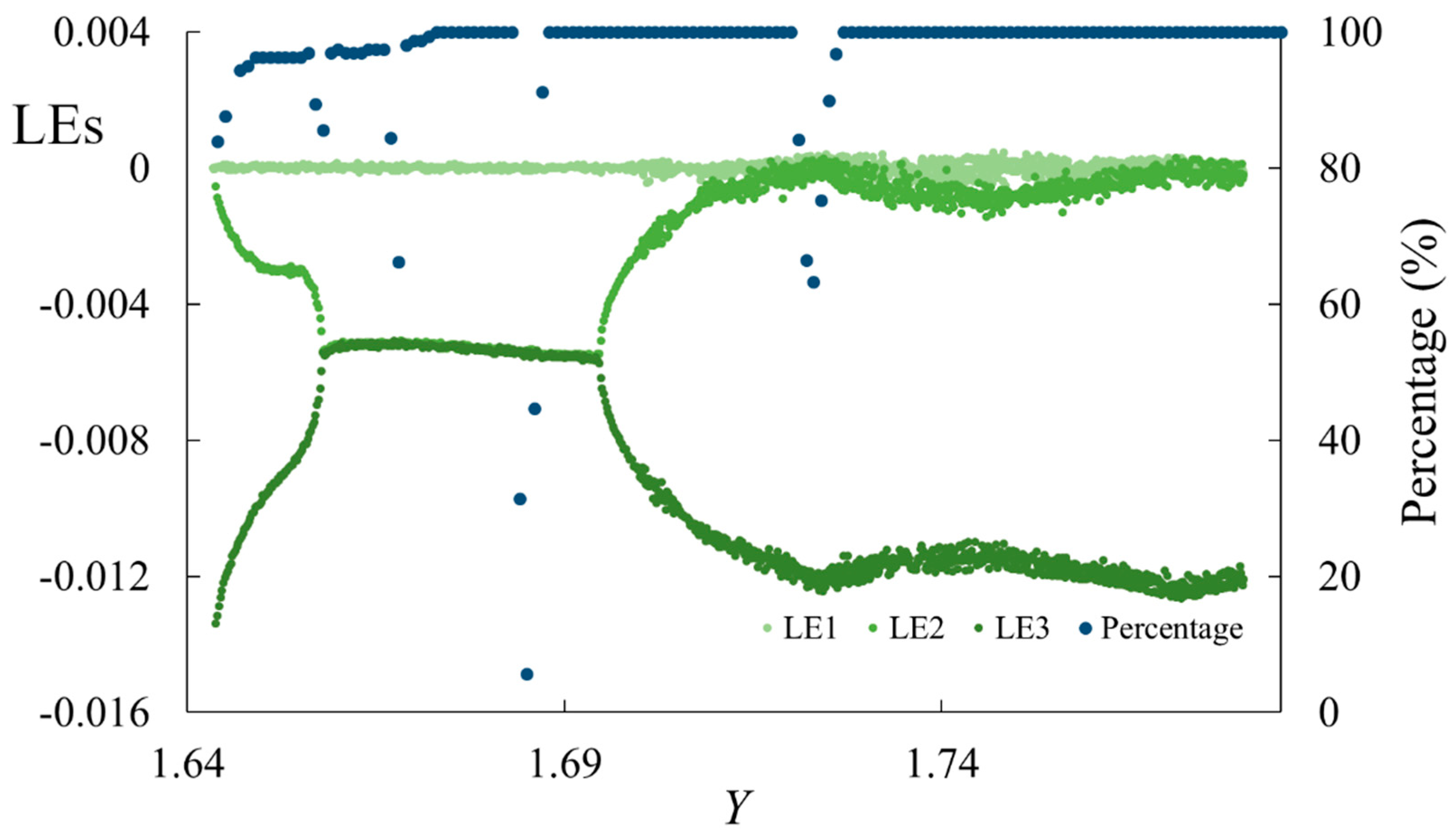
Originally, we believed that the apex of the symmetric-like bubble might be the ideal place to gain shift due to it having greater instability. However, the data shown in Figure 14 tells a different story. The system shows an instability at a location that seems to not match with the LEs. The dip at Y = 1.721 does not line up exactly with the apex of the symmetric-like bubble, instead, it is slightly to the right.
When we instead superimpose the gain shift with the LEs for C = 3.1 in Figure 15, we see a dip where the asymmetric bubble reaches its apex, the signatory two-zero LEs.
This tells us that, when the parameter shifts, we must consider the stability of the attractor at both the original parameter value and the shifted value. In other words, when the gain-shift method is applied, one needs to consider the attractor’s stability at both gains.
5. Conclusions
By power shifting, we can discover windows and access many attractors reliably even with noise on the frequency and a linear ramp on the injected signal amplitude of LIS. We select a base attractor which enhances the power shift’s reliability of accessing a desired attractor. Using the modified power-shift technique with the interim parameter shift, we expand access to attractors by temporarily modulating the gain (parameter), in this case. The power-shift method in conjunction with the interim parameter shift is attractive because it can be experimentally applied without significant or long-lasting modifications to the experimental system itself. When gain-shift results are compared to the LE patterns for a specific gain, we find critical points of the spectra where the attractor is unlikely to survive the gain shift. Noise and lag effects obscure the power-shift technique minimally for large domain attractors. Small domain attractors are inaccessible. Experimentally, we believe that the enhanced power-shift method, which enables an experimentalist to both discover and access coexisting attractors, is appealing because this provides flexibility to move from one type of system dynamics to another. By varying other system parameters, this method could facilitate, for example, a mapping of the dynamical states in parameters space of frequency detuning [7].
The Lyapunov exponents continue to herald system dynamics, attractor and window domains, and the level of instability associated with the various patterns. We know, for example, that every attractor has a unique LE pattern that is choreographed by the subtle variations of the attractor dynamics and are circumscribed by converging and diverging LE spectral patterns including the signature two-zero LEs at the origin and demise of the attractor [37]. We understand symmetric-like and asymmetric bubbles as imminent bifurcations and existing bifurcations, respectively. These results reiterate the universality of the LEs spectra patterns. There are still unknown patterns observed in other nonlinear systems which need to be defined that may or may not be associated with the LIS systems, but what we do know, is that the Lyapunov spectra has many mysteries yet to be discovered.
The power-shift method, along with the interim gain shift, is an answer to the question of how to access individual attractors stably and accurately even under experimental conditions. Identifying the dominance of one attractor over another in the same system and understanding the conditions that might change this dominance remains an open issue.
Author Contributions
Conceptualization, J.R.H., E.K.T.B., D.M.C. and D.K.B.; methodology, E.K.T.B., J.R.H.; Software, D.M.C., E.K.T.B., J.R.H.; Data Curation, E.K.T.B., J.R.H. and D.M.C.; writing—original draft preparation, D.K.B.; writing—review and editing, E.K.T.B., J.R.H., D.M.C. and D.K.B.; Visualization, J.R.H.; Supervision, D.K.B. All authors have read and agreed to the published version of the manuscript.
Funding
The APC was funded by MDPI AG.
Data Availability Statement
Data available on request. The data presented in this study are available on request from the corresponding author.
Acknowledgments
We are grateful to Al Rosenberger for his experimental acumen and consultations. We thank Corey Paulson and Camryn Paulson for their valuable computations.
Conflicts of Interest
The authors declare no conflict of interest.
Appendix A
We describe the procedure to discover attractors and windows using the power-shift method:
- Create m identical sequences of input signal amplitudes by dividing the domain ΔY into n equally spaced Y values and then randomize the order of each sequence. This creates multiple, completely arbitrary sequences of the same number set, Yji (I =1, 2, ..., n), (j = 1, 2, …, m);
- Power shift through the domain of the first random sequence of ΔY. To do this, begin the process at Y11, evolve the system for T units of time to stabilize the trajectory on a specific orbit (an attractor’s characteristic phase space);
- Record the final conditions of the laser variables and control parameter;
- Repeat steps 2 and 3 until all m sequences are recorded;
- Reorder all m sequences and compare the dynamics found at each input power, any discrepancies imply coexistence
Appendix B
Table A1 summarizes the results of the power-shift method without noise or a linear ramp added to the injected signal. This table provides a way to access the known attractor in LIS solely power shifting.
We discuss the results of the study of the power- shift method without noise by starting with the two simplest goal attractors, AI and AII. There is no coexisting attractor for AI and only one attractor (AIV) with a narrow domain of existence coexists with AII for the region 1.275 < Y < 1.6. One can select any base attractor (AI-AVIII) using any Y0 and TAP, then power shift at YPS ≤ 1 to access AI and the power shift at YPS = 1.54 to access AII.

Table A1.
LIS Attractor Access Via a Power Shift YPS.
| Goal Attractor | Base Attractor | Base Period (τ) | Y0 | YPS | TAP ± Leeway |
|---|---|---|---|---|---|
| AI | Any | Any | |||
| AII | Any | Any | 1.54 | Any | |
| AIII | AII | 108.025 | 1.51 * | 1.8 | 8 ± 52 |
| AIV | AI | 63.132 | 0.854 | 1.114 | 3 ± 4 |
| AV | AIII | 163.551 | 1.63 * | 1.84 | 151 ± 50 |
| AVI | AIII | 158.396 | 1.72 * | 1.96 | 154 ± 27 |
| AVII | AIII | 156.964 | 1.8 | 1.269 | 138 ± 2 |
* Y0 optimized using the method performed in Figure 7.
References
- Bonifacio, R.; Lugiato, L.A. Cooperative effects and bistability for resonance fluorescence. Opt. Commun. 1976, 19, 172–176. [Google Scholar] [CrossRef]
- Bonifacio, R.; Lugiato, L.A. Mean field model for absorptive and dispersive bistability with inhomogeneous broadening. Lett. Nuovo Cimento 1978, 21, 517–521. [Google Scholar] [CrossRef]
- Erneux, T.; Gavrielides, A.; Kovanis, V. Low pump stability of an optically injected diode laser. Quantum Semiclassical Opt. J. Eur. Opt. Soc. Part B 1997, 9, 811–818. [Google Scholar] [CrossRef]
- Wieczorek, S.; Simpson, T.B.; Krauskopf, B.; Lenstra, D. Bifurcation transitions in an optically injected diode laser: Theory and experiment. Opt. Commun. 2003, 215, 125–134. [Google Scholar] [CrossRef] [Green Version]
- Tchinda, T.; Njitacke, Z.; Fozin Fonzin, T.; Fotsin, H. Dynamics of an optically injected diode laser subject to periodic perturbation: Occurrence of a large number of attractors, bistability and metastable chaos. CSSP 2019, 8, 66. [Google Scholar] [CrossRef]
- Lingnau, B.; Chow, W.W.; Schöll, E.; Lüdge, K. Feedback and injection locking instabilities in quantum-dot lasers: A microscopically based bifurcation analysis. New J. Phys. 2013, 15, 093031. [Google Scholar] [CrossRef]
- Jiang, Z.-F.; Wu, Z.-M.; Jayaprasath, E.; Yang, W.-Y.; Hu, C.-X.; Xia, G.-Q. Nonlinear dynamics of exclusive excited-state emission quantum dot lasers under optical injection. Photonics 2019, 6, 58. [Google Scholar] [CrossRef] [Green Version]
- Lugiato, L.A.; Narducci, L.M.; Bandy, D.K.; Pennise, C.A. Breathing, spiking and chaos in a laser with injected signal. Opt. 1983, 46, 64–68. [Google Scholar] [CrossRef]
- Bandy, D.K.; Narducci, L.M.; Lugiato, L.A. Coexisting attractors in a laser with an injected signal. JOSA B 1985, 2, 148–155. [Google Scholar] [CrossRef]
- Jones, D.J.; Bandy, D.K. Attractors and chaos in the laser with injected signal. J. Opt. Soc. Am. B 1990, 7, 2119. [Google Scholar] [CrossRef]
- Gallas, J.A.C. Structure of the parameter space of the Hénon map. Phys. Rev. Lett. 1993, 70, 2714–2717. [Google Scholar] [CrossRef] [PubMed]
- Bonatto, C.; Garreau, J.C.; Gallas, J.A.C. Self-similarities in the frequency-amplitude space of a loss-modulated CO2 laser. Phys. Rev. Lett. 2005, 95, 143905. [Google Scholar] [CrossRef] [Green Version]
- Bonatto, C.; Gallas, J.A.C. Accumulation horizons and period adding in optically injected semiconductor lasers. Phys. Rev. E 2007, 75, 055204. [Google Scholar] [CrossRef] [PubMed] [Green Version]
- Guckenheimer, J.; Holmes, P. Nonlinear Oscillations, Dynamical Systems, and Bifurcations of Vector Fields; Springer: New York, NY, USA, 1983. [Google Scholar]
- Haken, H. Synergetics: An Introduction; Springer: New York, NY, USA, 1983. [Google Scholar]
- Schuster, H.G.; Just, W. Deterministic Chaos: An Introduction, 4th ed.; Wiley-VCH: Berlin, Germany, 2005. [Google Scholar]
- Narducci, L.M.; Abraham, N.B. Laser Physics and Laser Instabilities; World Scientific: Singapore, 1980. [Google Scholar]
- Rössler, O.E. An equation for continuous chaos. Phys. Lett. A 1976, 57, 397–398. [Google Scholar] [CrossRef]
- Shaw, R. Strange attractors, chaotic behavior, and information flow. Z. Für Nat. A 1981, 36, 80–112. [Google Scholar] [CrossRef]
- Mandelbrot, B.B. The Fractal Geometry of Nature; Henry Holt and Company: New York, NY, USA, 1983; ISBN 978-0-7167-1186-5. [Google Scholar]
- Eckmann, J.-P.; Ruelle, D. Ergodic theory of chaos and strange attractors. In The Theory of Chaotic Attractors; Hunt, B.R., Li, T.-Y., Kennedy, J.A., Nusse, H.E., Eds.; Springer: New York, NY, USA, 2004; pp. 273–312. ISBN 978-0-387-21830-4. [Google Scholar]
- Thompson, J.M.T.; Stewart, H.B. Nonlinear Dynamics and Chaos: Geometrical Methods for Engineers and Scientists; Wiley: Hoboken, NJ, USA, 1986; ISBN 978-0-471-90960-6. [Google Scholar]
- Gibbs, H.M.; Hopf, F.A.; Kaplan, D.L.; Shoemaker, R.L. Observation of chaos in optical bistability. Phys. Rev. Lett. 1981, 46, 474–477. [Google Scholar] [CrossRef]
- Arecchi, F.T.; Meucci, R.; Puccioni, G.; Tredicce, J. Experimental evidence of subharmonic bifurcations, multistability, and turbulence in a Q-Switched gas laser. Phys. Rev. Lett. 1982, 49, 1217–1220. [Google Scholar] [CrossRef]
- Tredicce, J.R.; Arecchi, F.T.; Puccioni, G.P.; Poggi, A.; Gadomski, W. Dynamic behavior and onset of low-dimensional chaos in a modulated homogeneously broadened single-mode laser: Experiments and theory. Phys. Rev. A 1986, 34, 2073–2081. [Google Scholar] [CrossRef]
- Dangoisse, D.; Glorieux, P.; Hennequin, D. Laser chaotic attractors in crisis. Phys. Rev. Lett. 1986, 57, 2657–2660. [Google Scholar] [CrossRef]
- Dangoisse, D.; Glorieux, P.; Hennequin, D. Chaos in a CO2 laser with modulated parameters: Experiments and numerical simulations. Phys. Rev. A 1987, 36, 4775–4791. [Google Scholar] [CrossRef]
- Derozier, D.; Bielawski, S.; Glorieux, P. Dynamical behavior of a doped fiber laser under pump modulation. Opt. Commun. 1991, 83, 97–102. [Google Scholar] [CrossRef]
- Meucci, R.; Poggi, A.; Arecchi, F.T.; Tredicce, J.R. Dissipativity of an optical chaotic system characterized via generalized multistability. Opt. Commun. 1988, 65, 151–156. [Google Scholar] [CrossRef]
- Ott, E.; Grebogi, C.; Yorke, J.A. Controlling chaos. Phys. Rev. Lett. 1990, 64, 1196–1199. [Google Scholar] [CrossRef] [PubMed]
- Pyragas, K. Continuous control of chaos by self-controlling feedback. Phys. Lett. A 1992, 170, 421–428. [Google Scholar] [CrossRef]
- Li, C.; Sprott, J.C. Finding coexisting attractors using amplitude control. Nonlinear Dyn. 2014, 78, 2059–2064. [Google Scholar] [CrossRef]
- Li, C.; Wang, X.; Chen, G. Diagnosing multistability by offset boosting. Nonlinear Dyn. 2017, 90, 1335–1341. [Google Scholar] [CrossRef]
- Burton, E.K.T.; Hall, J.R.; Chapman, D.M.; Bandy, D.K. Shifts in control parameter dynamically access individual attractors in a multistable system. Nonlinear Dyn. 2021, 105, 1877–1883. [Google Scholar] [CrossRef]
- Gu, Y.; Bandy, D.K.; Yuan, J.-M.; Narducci, L.M. Bifurcation routes in a laser with injected signal. Phys. Rev. A 1985, 31, 354–360. [Google Scholar] [CrossRef]
- Bandy, D.K.; Hall, J.R.; Denker, M.E. Predicting the evolutionary dynamic behavior of a laser with injected signal using Lyapunov exponents. Phys. Rev. A 2015, 92, 013841. [Google Scholar] [CrossRef]
- Bandy, D.K.; Burton, E.K.T.; Hall, J.R.; Chapman, D.M.; Elrod, J.T. Predicting attractor characteristics using Lyapunov exponents in a laser with injected signal. Chaos Interdiscip. J. Nonlinear Sci. 2021, 31, 013120. [Google Scholar] [CrossRef]
- Weiss, C.O. Instabilities and Chaotic Emission of Far-Infrared NH3-Lasers; Abraham, N.B., Chrostowski, J., Eds.; American Institute of Physics: Quebec City, QC, Canada, 1986; Volume 0667, p. 26. [Google Scholar]
- Abraham, N.B.; Narducci, L.M. Laser Physics & Laser Instabilities; World Scientific Publishing Company: Singapore, 1988; ISBN 978-9971-5-0063-4. [Google Scholar]
- Abarbanel, H.D.I.; Brown, R.; Kadtke, J.B. Prediction and system identification in chaotic nonlinear systems: Time series with broadband spectra. Physics Letters A 1989, 138, 401–408. [Google Scholar] [CrossRef]
- Abarbanel, H.D.I.; Brown, R.; Kadtke, J.B. Prediction in chaotic nonlinear systems: Methods for time series with broadband Fourier spectra. Phys. Rev. A 1990, 41, 1782–1807. [Google Scholar] [CrossRef] [PubMed]
- Abarbanel, H.D.I.; Brown, R.; Kennel, M.B. Variation of Lyapunov exponents on a strange attractor. J. Nonlinear Sci. 1991, 1, 175–199. [Google Scholar] [CrossRef]
- Benettin, G.; Galgani, L.; Strelcyn, J.-M. Kolmogorov entropy and numerical experiments. Phys. Rev. A 1976, 14, 2338–2345. [Google Scholar] [CrossRef]
- Mandel, P.; Erneux, T. Laser Lorenz Equations with a time-dependent parameter. Phys. Rev. Lett. 1984, 53, 1818–1820. [Google Scholar] [CrossRef]
Figure 1.
Schematic of the global behavior of LIS is shown for parameters C = 3, = 0.5, = 0.1, = 0.01, Φ/ = −0.5. 1P, 2P, etc. denote limit cycles; AI-AVIII are individual attractors and WI and WII are periodic windows in chaos; C is chaos; vertical arrows represent attractor transitions. The hashed rectangle (in yellow) indicates the Y domain where AII, AIII, and AV coexist. The asterisk * indicates the transition from AVI to AII at Y = 1.948.
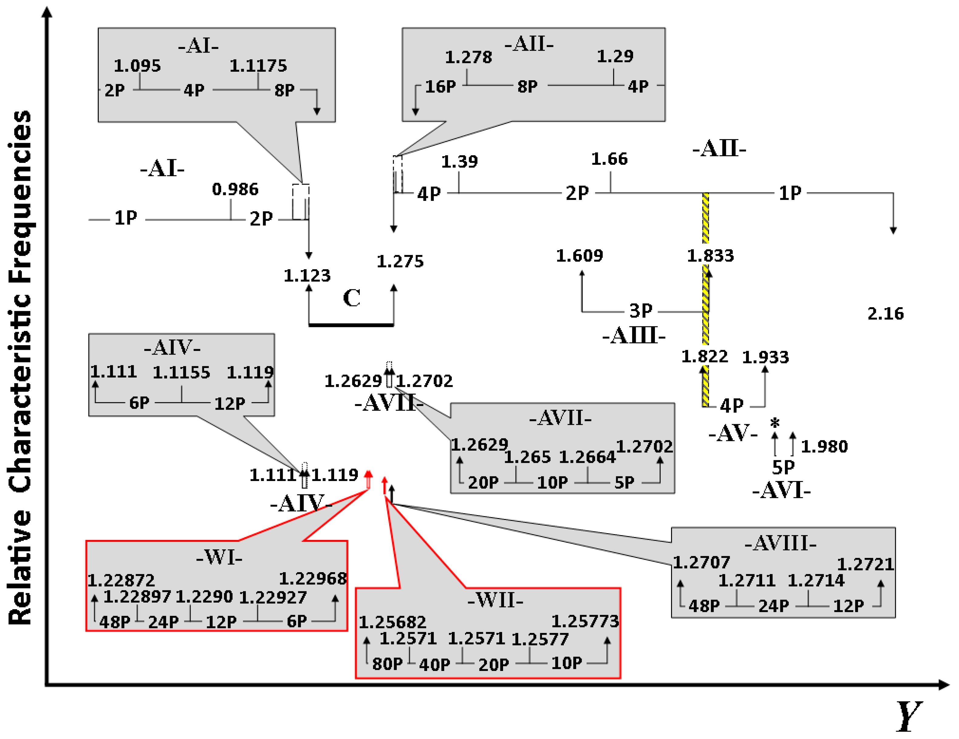
Figure 2.
(a) Global view of 3 attractor domains using the first 3 LEs as a function of the injected field Y, AII coexists with AIII, AV, and AVI (domains D, E, and F respectively); Chaos coexists with AVII and AVIII (domains B and C, respectively); and AI coexists with AIV (domain A). (b) is AIV, (c) is AVII, and (d) is AVIII.

Figure 3.
LEs are graphed as a function Y. Lyapunov spectra are plotted in the forward (black) and backward (red) scans for (a) WI and (b) WII. Note, the regions where red and black dots do not override each other.
Figure 3.
LEs are graphed as a function Y. Lyapunov spectra are plotted in the forward (black) and backward (red) scans for (a) WI and (b) WII. Note, the regions where red and black dots do not override each other.
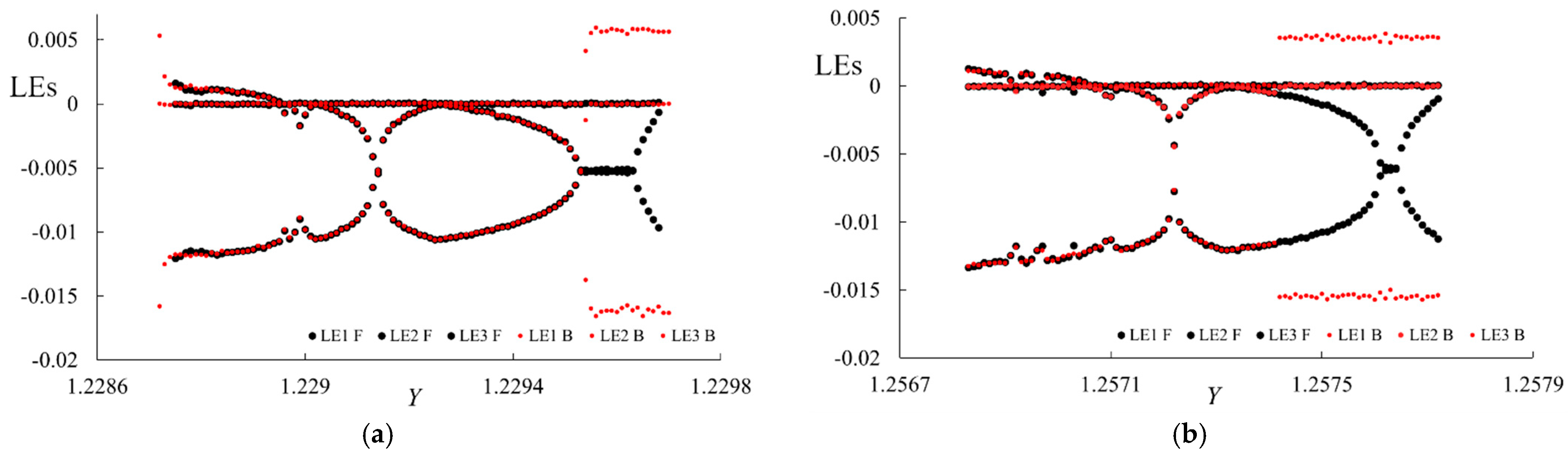
Figure 4.
The axes are Re|X|, Im|X|, and D. The magenta x marks the power shift location, the base attractor AVI. (a) Down shift from AVI (in green) at Y0 = 1.96 to AV (in blue) at YPS = 1.84. (b) Down shift from AVI (in green) at Y0 = 1.96 to AII (in blue) at YPS = 1.84.
Figure 4.
The axes are Re|X|, Im|X|, and D. The magenta x marks the power shift location, the base attractor AVI. (a) Down shift from AVI (in green) at Y0 = 1.96 to AV (in blue) at YPS = 1.84. (b) Down shift from AVI (in green) at Y0 = 1.96 to AII (in blue) at YPS = 1.84.
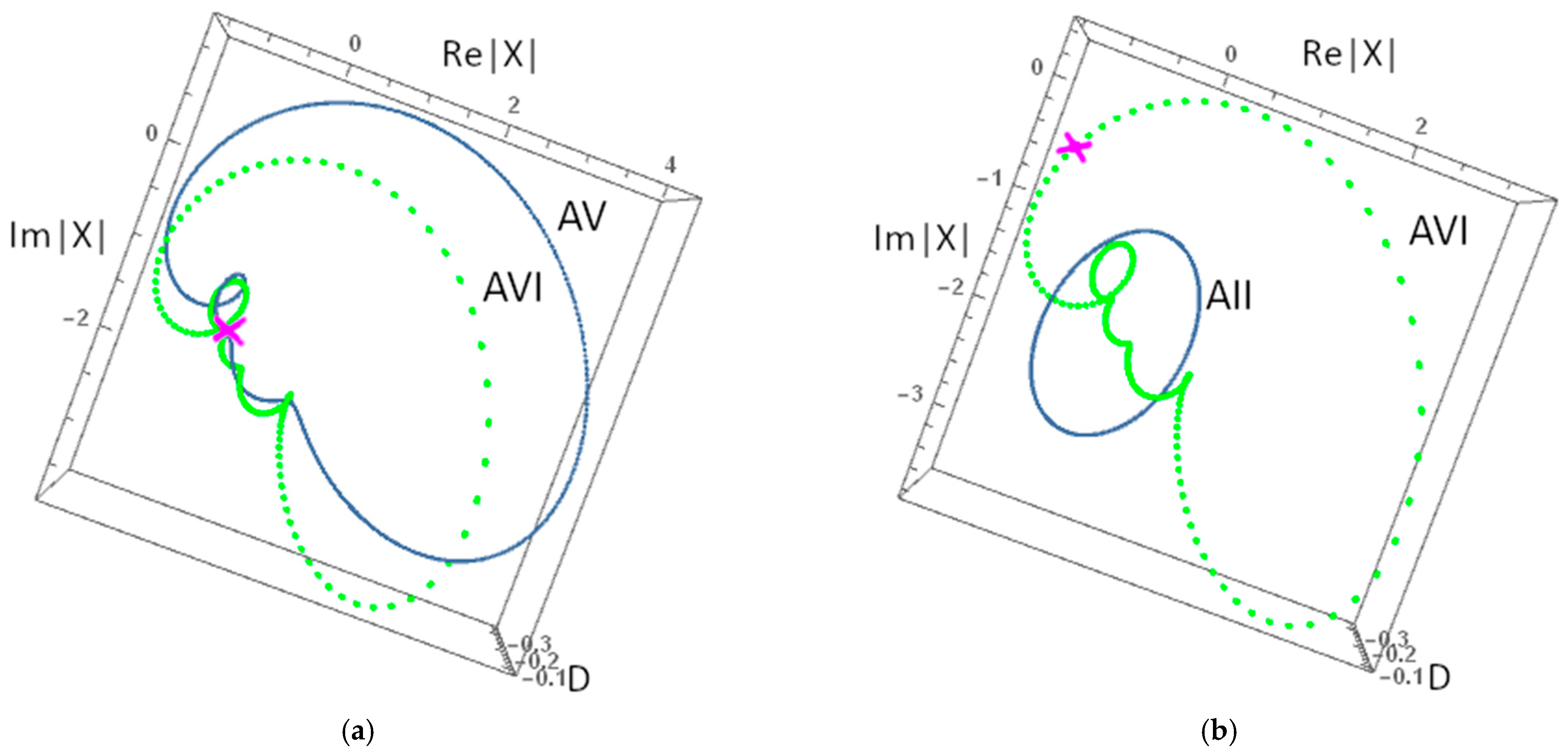
Figure 5.
Schematic of LEs vs Y graphed over the partial domains of AIII and AV at different values of the gain, C. (a–c) AIII, the gain changes 2.7, 3.0, 3.1, respectively. (d–f) AV, the gain changes 3.0, 3.1, 3.2, respectively.
Figure 5.
Schematic of LEs vs Y graphed over the partial domains of AIII and AV at different values of the gain, C. (a–c) AIII, the gain changes 2.7, 3.0, 3.1, respectively. (d–f) AV, the gain changes 3.0, 3.1, 3.2, respectively.
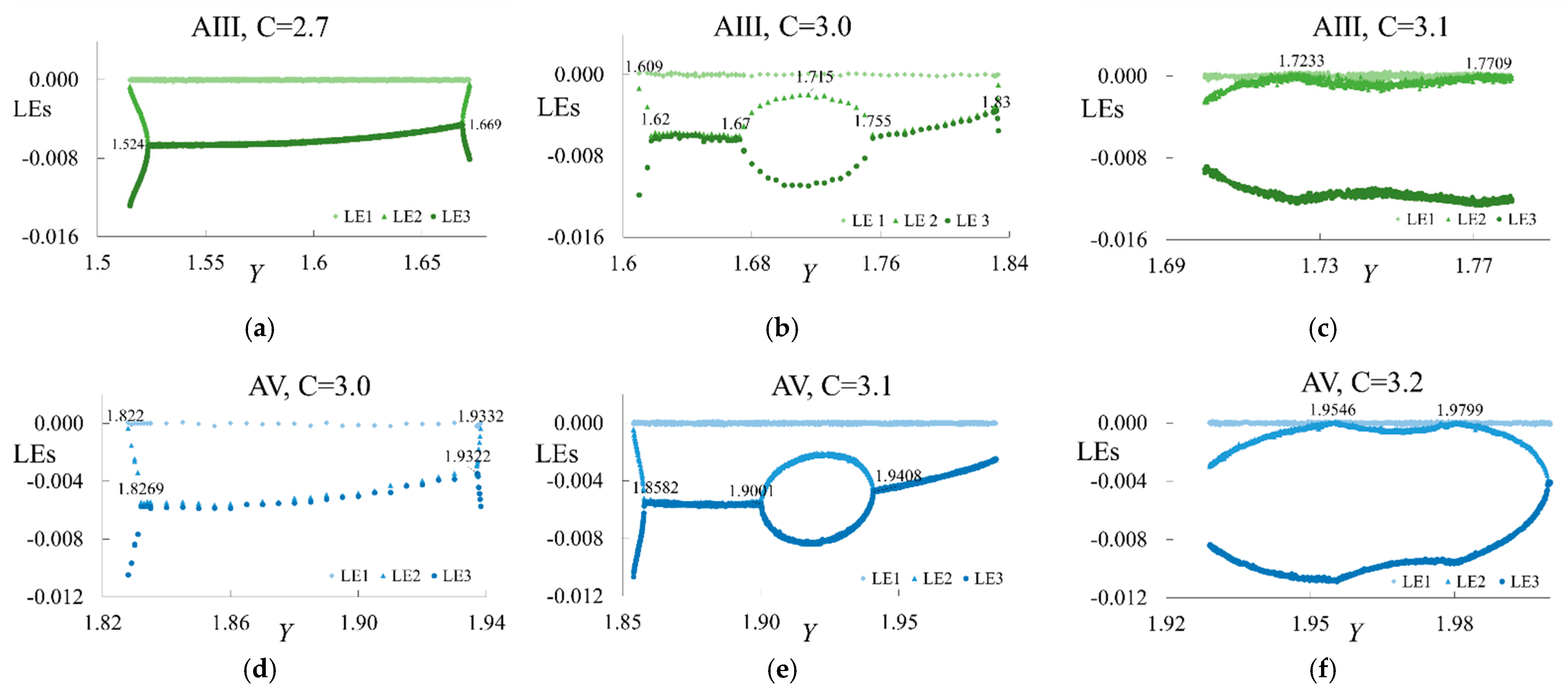
Figure 6.
Schematic of LEs vs Y graphed over the domains of AVI at different values of the gain, C. (a–e) C = 3.0, 3.2, 3.25, 3.3, and 3.35, respectively.
Figure 6.
Schematic of LEs vs Y graphed over the domains of AVI at different values of the gain, C. (a–e) C = 3.0, 3.2, 3.25, 3.3, and 3.35, respectively.

Figure 7.
The plot for the largest time interval for each Y0 value in AIII which when power shifted to Yps = 1.84 (a) or YPS = 1.96 (b) takes the system to AV (a) or AVI (b), respectively. Y0 = 1.63 has the largest tranche for YPS = 1.84. Y0 = 1.72 has the largest tranche for YPS = 1.96.
Figure 7.
The plot for the largest time interval for each Y0 value in AIII which when power shifted to Yps = 1.84 (a) or YPS = 1.96 (b) takes the system to AV (a) or AVI (b), respectively. Y0 = 1.63 has the largest tranche for YPS = 1.84. Y0 = 1.72 has the largest tranche for YPS = 1.96.
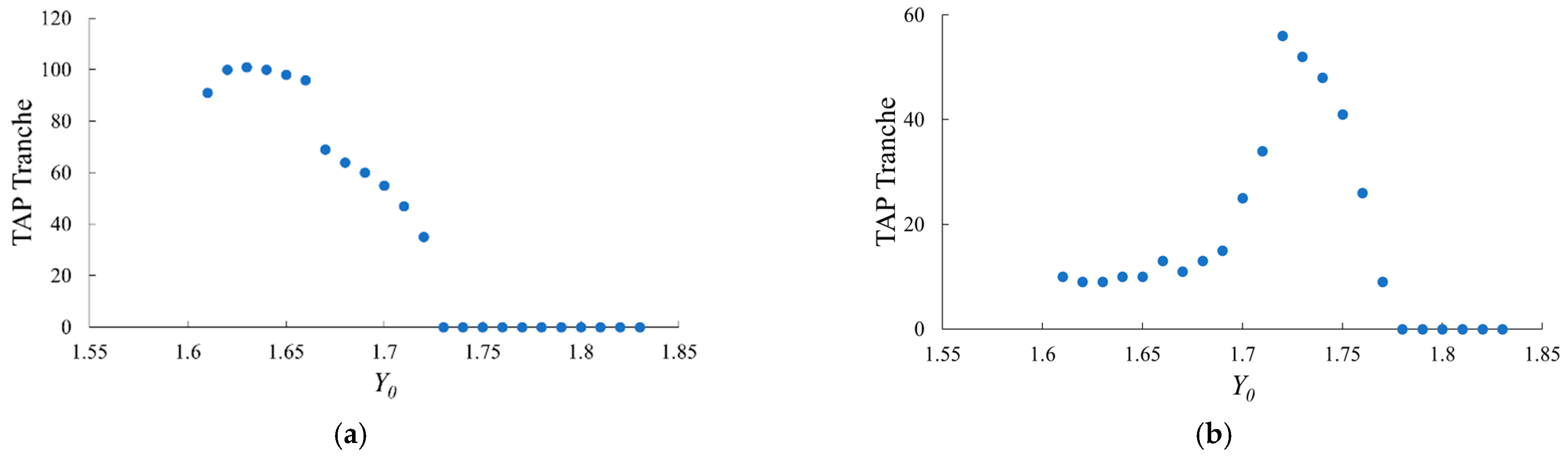
Figure 8.
Power-shift method from AIII at (a) Y0 = 1.63 transitioning to coexisting AII and AV via YPS = 1.84, and (b) Y0 = 1.72 transitioning to coexisting AII and AVI via YPS = 1.96.
Figure 8.
Power-shift method from AIII at (a) Y0 = 1.63 transitioning to coexisting AII and AV via YPS = 1.84, and (b) Y0 = 1.72 transitioning to coexisting AII and AVI via YPS = 1.96.
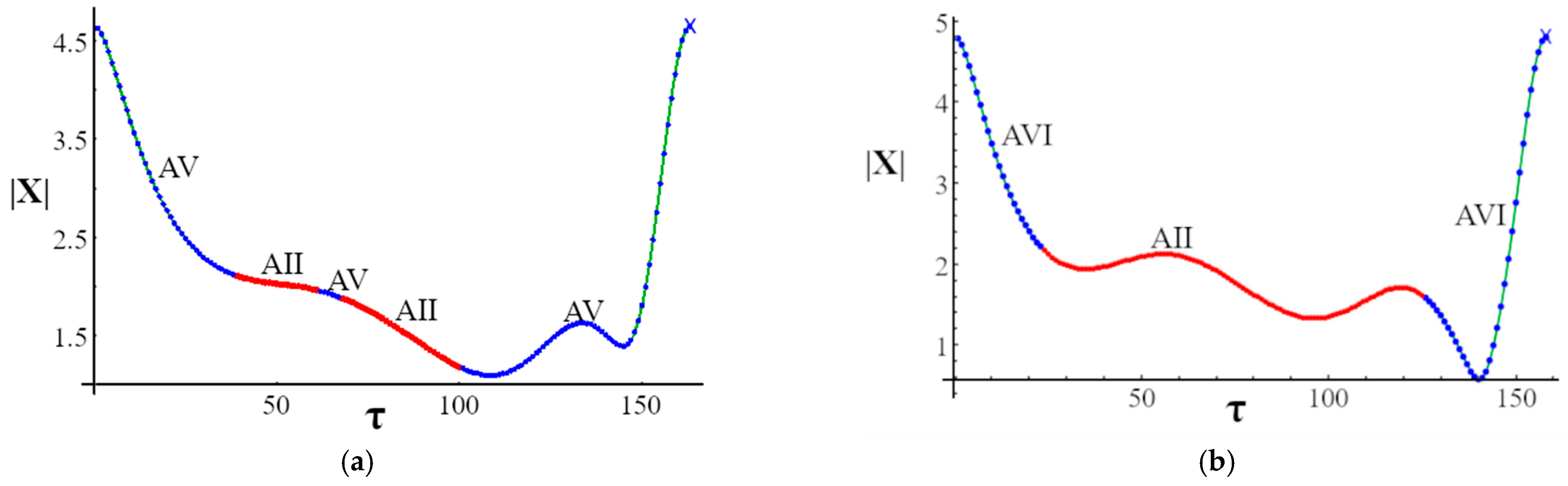
Figure 9.
Noise is added to the powershift method using a randomly generated noise for the frequency of the injected signal every 0.4τ with an amplitude range of ±0.0015. (a) Run 1 and (b) Run 2. Note, intermittent access to AII on the shoulder of the peak at 150τ compared to Figure 8a without noise.
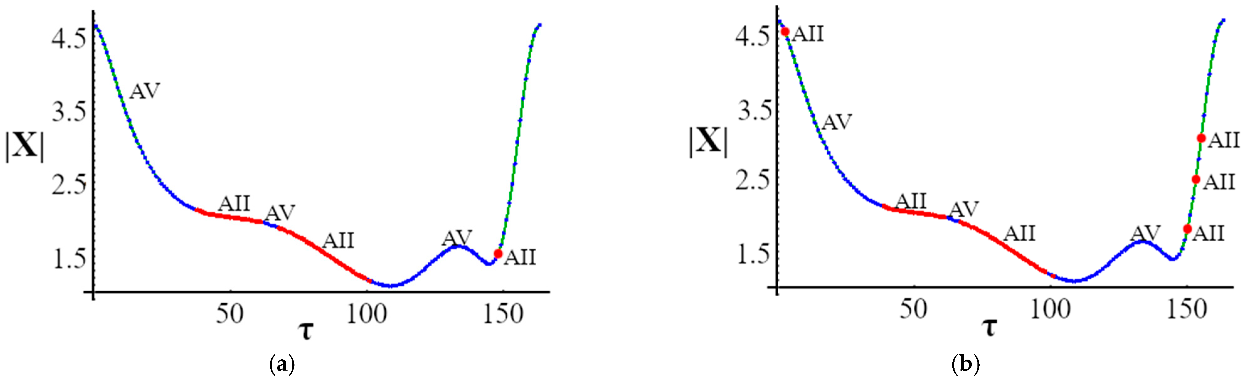
Figure 10.
Power-shift method applying a linear ramp with Tlag = 15, Y0 = 1.63 for base AIII with YPS = 1.84. The blue X marks the center of the largest time interval which power shift to AV. Two periods are displayed for clarity.
Figure 10.
Power-shift method applying a linear ramp with Tlag = 15, Y0 = 1.63 for base AIII with YPS = 1.84. The blue X marks the center of the largest time interval which power shift to AV. Two periods are displayed for clarity.
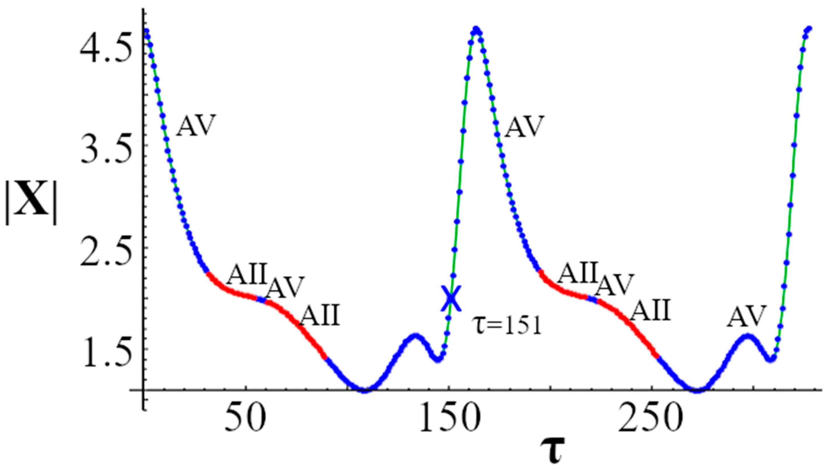
Figure 11.
Power-shift method applying a linear ramp with Tlag = 15 and noise with amplitude = ±0.0015, Y0 = 1.63 for base AIII with the YPS = 1.84.
Figure 11.
Power-shift method applying a linear ramp with Tlag = 15 and noise with amplitude = ±0.0015, Y0 = 1.63 for base AIII with the YPS = 1.84.
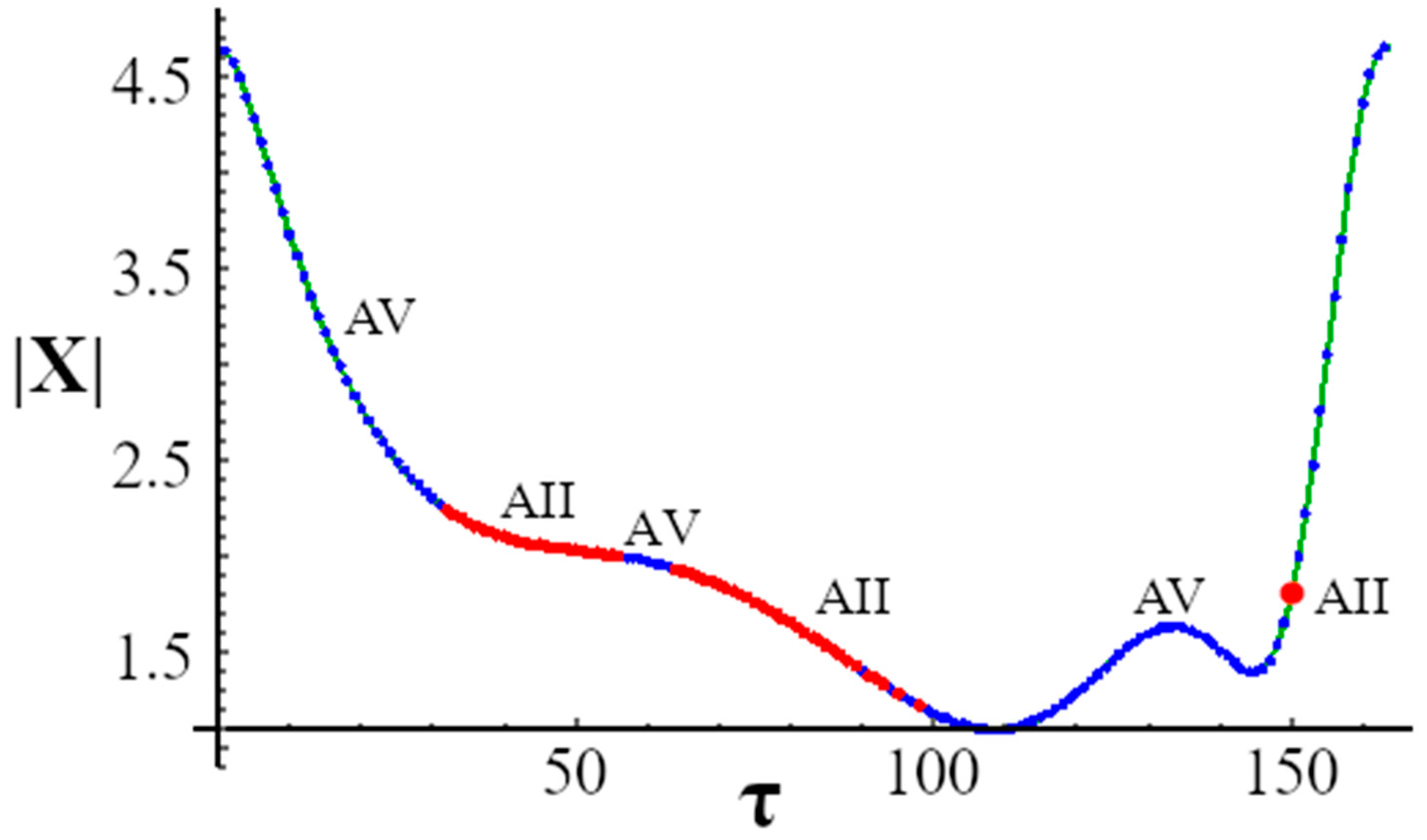
Figure 12.
The percentage chance that AIII survives the gain shift as a function of Y.
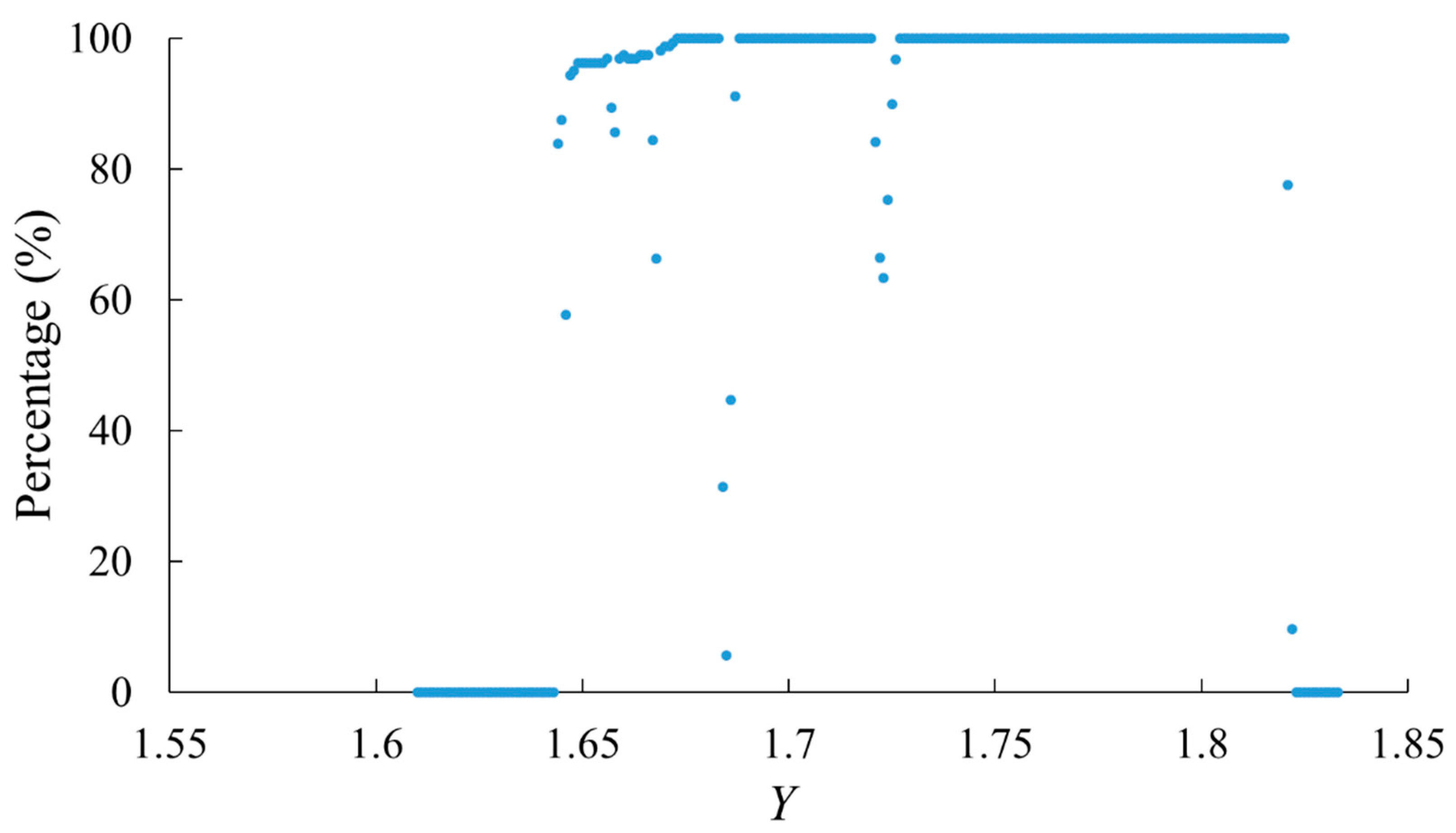
Figure 13.
Comparison of the power shift without a lag in blue dots and with Tlag = 15τ at Y0 = 1.63 for base AIII with YPS = 1.84 in orange xs. The vertical axis represents the resultant attractor for a power shift.
Figure 13.
Comparison of the power shift without a lag in blue dots and with Tlag = 15τ at Y0 = 1.63 for base AIII with YPS = 1.84 in orange xs. The vertical axis represents the resultant attractor for a power shift.
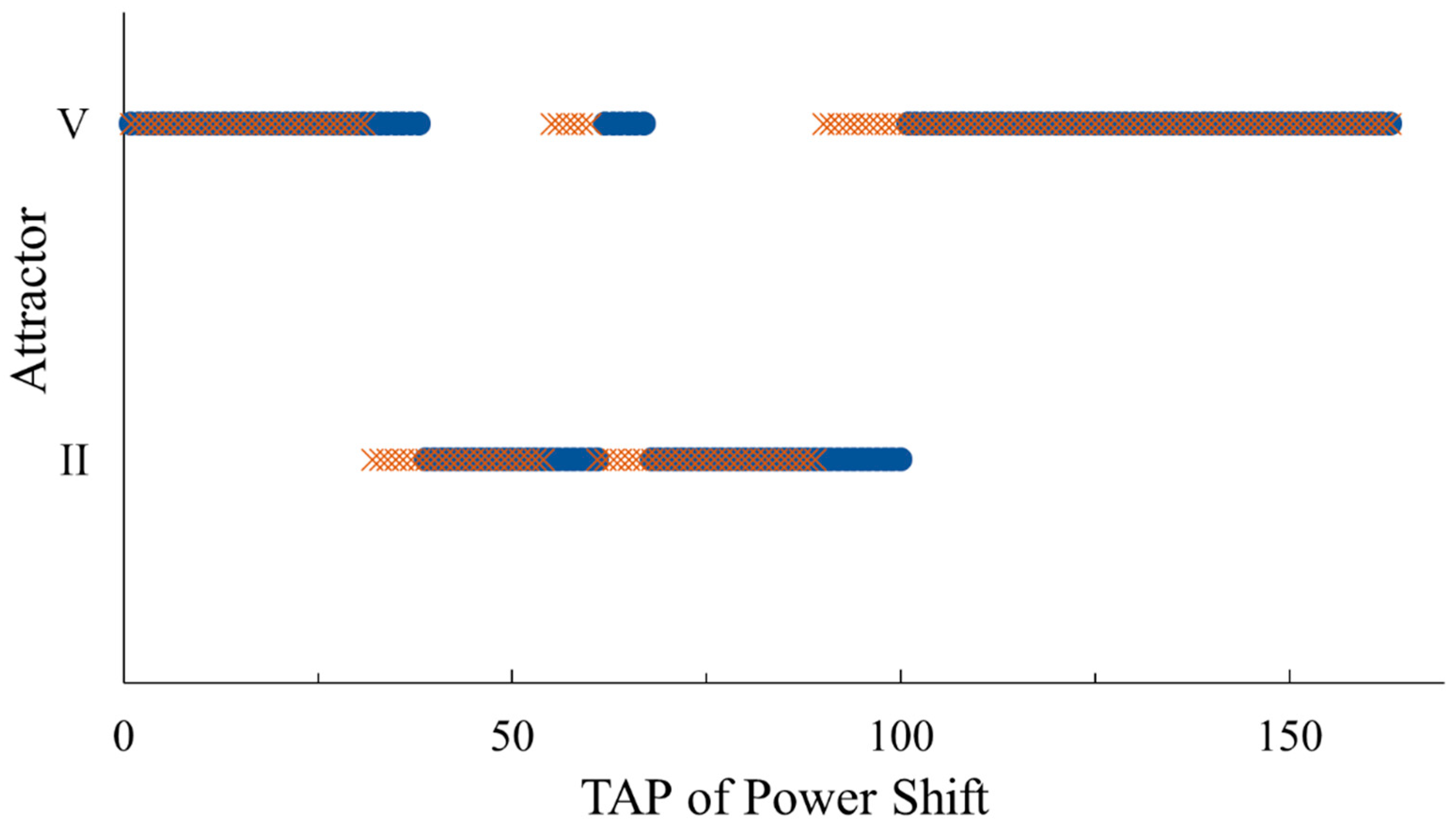
Figure 14.
Schematic of LEs vs Y graphed over the domain of AIII at C = 3.0 and overlayed with the gain shift results. The right ordinate displays the percentage of times that AIII survives the gain shift.
Figure 14.
Schematic of LEs vs Y graphed over the domain of AIII at C = 3.0 and overlayed with the gain shift results. The right ordinate displays the percentage of times that AIII survives the gain shift.
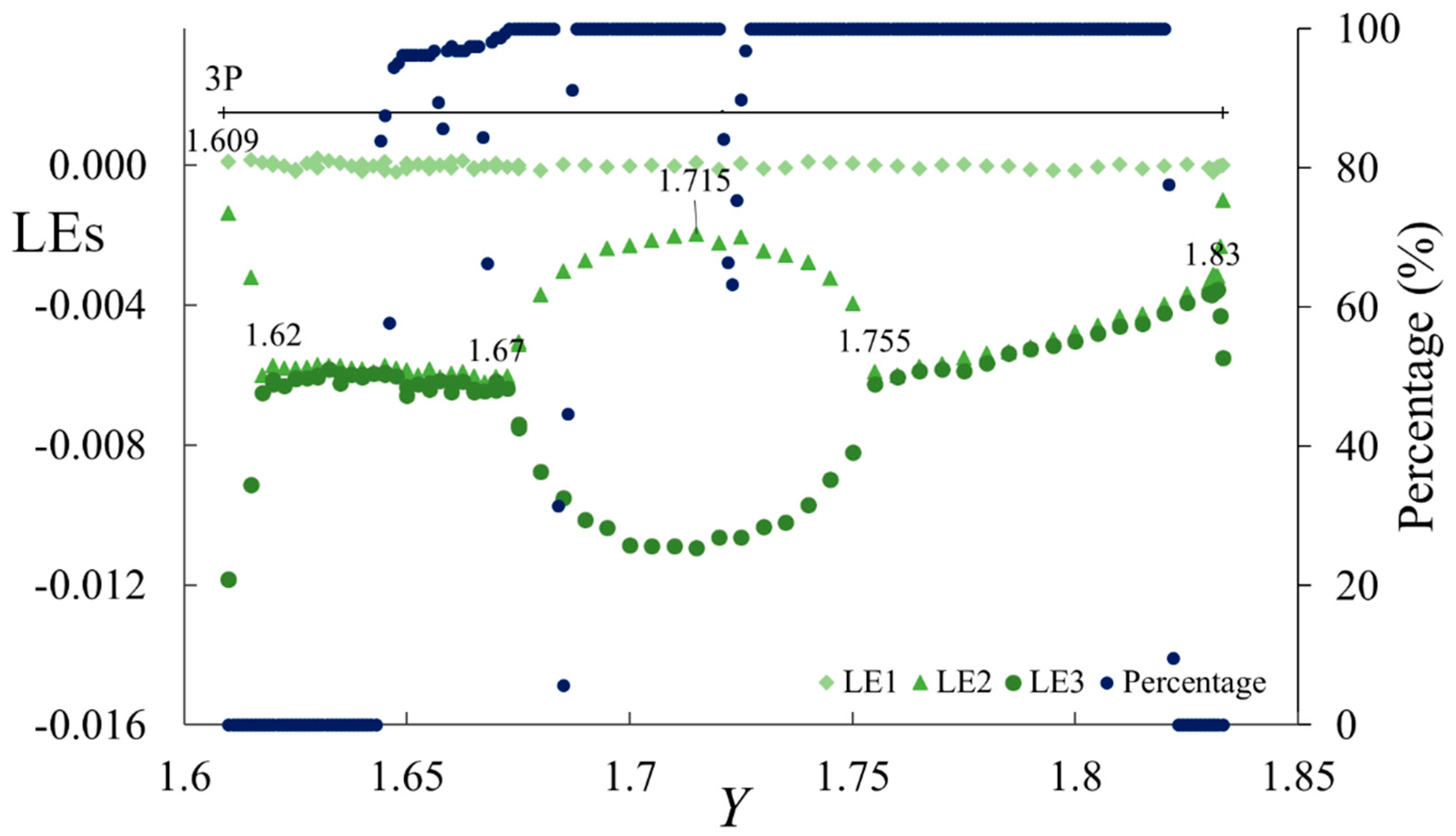
Figure 15.
Schematic of LEs vs Y graphed over the partial LE domain of AIII at C = 3.1 and overlayed with the gain-shift results. The right ordinate displays the percentage that AIII survives the gain shift.
Figure 15.
Schematic of LEs vs Y graphed over the partial LE domain of AIII at C = 3.1 and overlayed with the gain-shift results. The right ordinate displays the percentage that AIII survives the gain shift.
Publisher’s Note: MDPI stays neutral with regard to jurisdictional claims in published maps and institutional affiliations. |
© 2021 by the authors. Licensee MDPI, Basel, Switzerland. This article is an open access article distributed under the terms and conditions of the Creative Commons Attribution (CC BY) license (https://creativecommons.org/licenses/by/4.0/).
Share and Cite
MDPI and ACS Style
Hall, J.R.; Burton, E.K.T.; Chapman, D.M.; Bandy, D.K. Experimentally Viable Techniques for Accessing Coexisting Attractors Correlated with Lyapunov Exponents. Appl. Sci. 2021, 11, 9905. https://doi.org/10.3390/app11219905
AMA Style
Hall JR, Burton EKT, Chapman DM, Bandy DK. Experimentally Viable Techniques for Accessing Coexisting Attractors Correlated with Lyapunov Exponents. Applied Sciences. 2021; 11(21):9905. https://doi.org/10.3390/app11219905
Chicago/Turabian StyleHall, Joshua Ray, Erikk Kenneth Tilus Burton, Dylan Michael Chapman, and Donna Kay Bandy. 2021. "Experimentally Viable Techniques for Accessing Coexisting Attractors Correlated with Lyapunov Exponents" Applied Sciences 11, no. 21: 9905. https://doi.org/10.3390/app11219905
Note that from the first issue of 2016, this journal uses article numbers instead of page numbers. See further details here.