
Design of a Partially Grid-Connected Photovoltaic Microgrid Using IoT Technology


1
Department of Electrical Engineering, College of Engineering, Qassim University, Unaizah 56452, Saudi Arabia
2
Department of Electrical Engineering, Faculty of Engineering, Aswan University, Aswan 81542, Egypt
3
Department of Computer Science, Hekma School of Engineering, Computing, and Informatics, Dar Al-Hekma University, Jeddah 22246, Saudi Arabia
4
Department of Future Technologies, University of Turku, 20520 Turku, Finland
5
Department of Technology, High Institute of Informatics and Mathematics, University of Monastir, Monastir 5000, Tunisia
*
Author to whom correspondence should be addressed.
Appl. Sci. 2021, 11(24), 11651; https://doi.org/10.3390/app112411651
Submission received: 2 November 2021
/
Revised: 24 November 2021
/
Accepted: 1 December 2021
/
Published: 8 December 2021
(This article belongs to the Topic Innovative Techniques for Smart Grids)
Abstract
:This study describes the design and control algorithms of an IoT-connected photovoltaic microgrid operating in a partially grid-connected mode. The proposed architecture and control design aim to connect or disconnect non-critical loads between the microgrid and utility grid. Different components of the microgrid, such as photovoltaic arrays, energy storage elements, inverters, solid-state transfer switches, smart-meters, and communication networks were modeled and simulated. The communication between smart meters and the microgrid controller is designed using LoRa communication protocol for the control and monitoring of loads in residential buildings. An IoT-enabled smart meter has been designed using ZigBee communication protocol to evaluate data transmission requirements in the microgrid. The loads were managed by a proposed under-voltage load-shedding algorithm that selects suitable loads to be disconnected from the microgrid and transferred to the utility grid. The simulation results showed that the duty cycle of LoRa and its bit rate can handle the communication requirements in the proposed PV microgrid architecture.
1. Introduction
Electric power systems have been developed over the past century until they became integrated systems in terms of planning, management, operation, and control. These systems are characterized by central bulk power generation power plants connected to consumers through high-, medium-, and low-voltage transmission and distribution networks. This complex power system forms the backbone of modern human civilization. The existing infrastructure uses strategies and technologies that were developed many decades ago, which utilize limited control and digital communication technologies of the 21st century [1]. Moreover, climate change concerns and environmental issues urged many countries to adopt new strategies for reducing the dependency on fossil fuels to reduce carbon dioxide emissions. Clean energy production is achieved through enabling renewable energy generation and integration into electrical energy systems. Power systems need to meet changes in generation profiles to create intelligent tools that rely on advanced sensors, ICT (information and communication technologies), and digital control technologies that can distribute electricity effectively, economically, and securely.
Renewable power integration can provide many advantages such as lowering cost and increasing system reliability, power quality, and energy efficiency [2,3]. The integration of renewables is achieved in the form of either mega-sized renewable energy parks connected to the main grid or small-sized units connected to distribution systems. Besides these, other forms of distributed small-size energy resources include fuel cells, microturbines, reciprocating engines, storage systems, and controllable loads. Such power generation resources require power-electronic interfaces, communications, and control systems to deal with and dispatch within the constraints of the uncertainty of renewable generation [4]. The concept of a Smart Grid has emerged as the vision of the future generation of power systems [5]. The smart grid’s attributes can be summarized in the following [6]: (1) optimal cost electricity generation considering dispatchable demands, (2) maximizing low-carbon generation, (3) resiliency of both physical and cyber-attacks, (4) ensuring the best power quality for consumers, and (5) monitoring of components and devices to prevent component outages or even system blackouts. It is important to mention herein that the cost of an electric system blackout is very high and results in severe economic and social impacts [7].
Smart grid enabling requires innovative solutions and technologies that include digital smart meters, sensors, actuators, controllable charging, intelligent circuit interfaces, phasor measurements units, communication systems, cloud computing, wide and local area controllers, home automation, etc. [8]. Smart grid technologies and associated infrastructures continue to grow tremendously, which requires associated approaches and methods to improve system performance and energy efficiency [9]. Demand response (DR) is the most economical and reliable solution for smart power systems [9,10,11,12]. The IEEE Std. 2030.6–2016 defines the DR as: The participation of customers in electricity markets by changing their electricity consumption patterns in response to the price signals or incentive mechanisms from DR service providers. [13]. The DR implementation allows the use of electricity with changes in the customer’s load profile according to their needs. Also, it allows dealing with the variation of renewable energy sources (RES) generation [14]. The DR implementation is relying on advances in ICT [15]. The DR implementation offers many opportunities for market agents to provide cost-effective solutions [14,16]. Demand response programs involve a series of control strategies to fulfill both end-users as well as specific requirements. In a typical DR scheme, a balancing strategy could be implemented to provide load flexibility during stress periods of the grid. The implementation of DR is still limited due to the lack of deploying smart technologies as well as the corresponding regulations [17].
The current Saudi Electricity Company (SEC) billing structure still utilizes traditional flat tariffs with no incentive packages to decrease their demand during peaks. In a recent study, a pricing scheme that includes time-of-use tariffs (TOU) is discussed and analyzed [18,19,20]. The TOU could increase billing during summer to 42~57% higher. In this study, the households were assumed to respond in different ways: (1) regulate their thermostat set-point to lower air conditioning demand, (2) either shift unneeded appliances to different periods of the day, or (3) invest in energy measures. Meanwhile, the SEC has started an ambitious project towards digital transformation by installing 10 million smart meters throughout the Kingdom by the year 2021 G. The most interesting feature is that customers can access real-time data about their consumption and hence, adjust their consumption patterns as needed [21]. Furthermore, regulations and bylaws that govern small-scale photovoltaic integration into distribution systems have been approved by Electricity and Cogeneration Regulatory Authority’s Administrative [22]. This shows the Saudi Electricity Company’s commitment to the objectives of the Kingdom’s Vision 2030 on renewable and sustainable energy [23,24].
Smart grid systems rely heavily on communication facilities to function. Power-line communication, wireless mesh networks, Cellular, satellite communication, fiber-optics, and short-range communication, are among the communication technologies projected to be used in the smart grid. The use of modern communication technologies in the smart grid is influenced by a variety of factors including geographic locations, application requirements, regulations, environmental issues, pricing, security, reliability, and many other factors [25]. Since the smart grid is currently receiving widespread usage from modern communication technologies, cyber security has become more essential for secure practices [26,27]. The cyber security measures aim to prevent data eavesdropping, prevent hazardous malware from running on smart grid embedded devices in addition to protecting customer privacy. A cyber-physical system (CPS) generally consists of a three-layer architecture (application, communication, and physical sensor devices) considered to employ contemporary ICT to manage physical system components remotely. The current use of CPS has been extended to many vital sectors including: construction, transportation, E-health, military, and smart-grids [28].
The emerging internet of things (IoT) technology interconnects the CPS system whereas its architecture can be modeled as a multilayer system. Integration of IoT technology has provided comparable potentials and several benefits to the electricity industry [29]. The whole process of power generation, transmission, distribution, consumption, and management may be made more efficient and intelligent by integrating the IoT components in power system nodes. By making autonomous decisions and taking reliable actions based on monitored situations, the performance of these intelligent nodes can be greatly enhanced. They can also interact with each other and coordinate the efforts to more effectively achieve system-wide goals. Communication infrastructure is a vital element in the design of the microgrid. There are two types of information that need to be transmitted across the microgrid: control signals and raw data. Each category should be treated with a given quality of service (QoS) and security level. Furthermore, the transmission distance, frequency of transmissions, and cost are also key parameters that need to be accounted for to choose the suitable communication protocol [26,30]. Various reports have been published that compare and contrast the existing communication standards to fulfill the requirements for each smart grid application [31,32].
An IoT communication network comprises different layers such as application, security, transport, network, and link layer. The communication protocols at the link layer can be classified into three categories: (1) short-range protocols include Bluetooth and ZigBee, (2) medium-range protocols include Wi-Fi, 4G/LTE, and 5G, and (3) Long-range protocols include Narrowband-IoT (NB-IoT), and LoRa (Long Range). The LoRa network is a low-power wide-area network that uses the spread-spectrum modulation technique. In this work, the LoRa network is proposed to implement a microgrid architecture based on IoT connectivity.
A voltage-based droop control method for the transition from grid-connected mode to the standalone mode was developed in Refs. [33,34]. The authors of [35] designed (active-reactive power) PQ and (voltage-frequency) VF control algorithms to minimize voltage and current spikes, there predominantly appear when the microgrid is switched between grid-connected and islanded operating modes.
This manuscript is an extension of the work published in [36], by means of the following contributions:
- A proposed design of a partially grid-connected microgrid based on the IoT communication network.
- A comprehensive simulation model using Matlab/Simulink was designed to evaluate the performance of the load-shedding algorithm and the associated communication protocol.
- A prototype design of IoT-based smart meter using ZigBee communication protocol.
- A LoRa based communication network is proposed to link the smart meters with the microgrid controller.
The rest of the paper is organized as follows. Section 2 describes the operation, control, and modeling of modern microgrids. Section 3 demonstrates the simulation models and designs used to describe the control of each component in the PV microgrid. Section 4 elaborates the architecture and design of the IoT communication network in addition to the communication protocol requirements. Finally, Section 5 displays the results and discussion followed by the conclusions.
2. Microgrid Operation and Control
Normal operation of a power system requires a perfect balance of active and reactive powers between generation and load as given using:
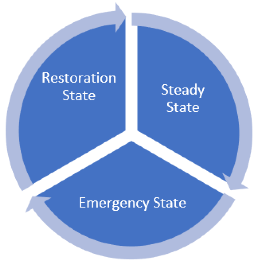
where PG and PL are the generated and load demand active power, respectively. QG and QL are the generated and load reactive power, respectively. Ng and NL are numbers of distributed generators and distributed loads, respectively. Ploss and Qloss are the active and reactive power losses, respectively. Also, there is a considerable power generation reserve that is used to compensate for any violation in generation scheduling during the operational planning phase. Basically, the power system involves continuous transition among three different states as shown in Figure 1. The steady state describes the normal operation of the electrical power system in which there will be a perfect balance of active and reactive powers between generation and demand. The frequency and voltage are used as the indicators for this balance and set to operate within specific allowable limits. The system operates in the emergency state for a specific time according to the type and nature of the disturbance. The emergency state involves a change in either voltage or frequency beyond the allowable limits. The power system control includes mechanisms that respond by fixing the problems and providing restorative actions that may include isolating faulted parts or shedding some loads from the system.
Microgrids are quite different from classical power systems due to the intermittent nature of generation resources. The operation of microgrids in both grid-connected and islanded modes has been investigated in the literature [37,38,39]. Microgrid operation emphasizes the supply of critical loads during power outages. In this case, some loads are usually disconnected using shedding algorithms that are classified into three main types namely: traditional, semi-adaptive, and adaptive algorithms [37]. The under voltage load shedding (UVLS) algorithm is simple to use and widely used in the literature [40,41,42,43]. In this paper, the UVLS algorithm is used to initiate the load shedding process. However, instead of disconnecting the load from the microgrid, it is transferred to the grid using fast solid-state transfer switches controlled by wireless signals transmitted through a LoRaWAN network and IoT control.
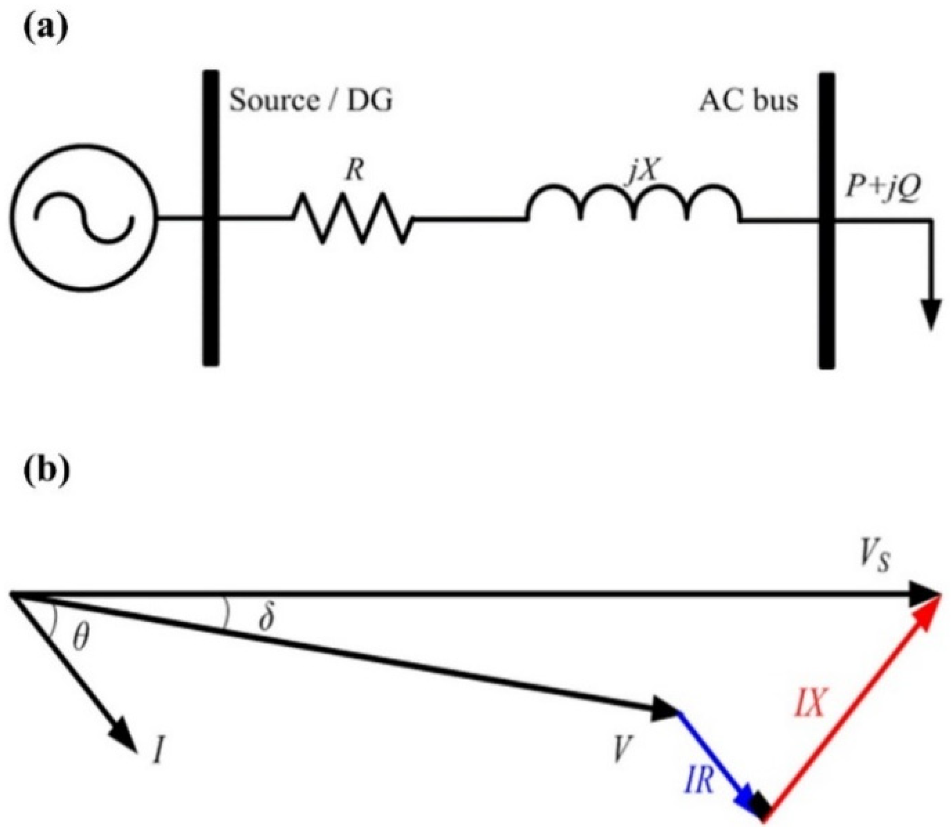
Figure 2a shows a simple two-node system with a source or a distributed generation (DG) unit, which feeds a reactive power load through a line segment of resistance and reactance R and X, respectively [44]. Since the load is a reactive power load, the current is lagging the voltage at the load terminal by an angle Hence, the source voltage must lead the load voltage by an angle , which is usually referred to as the torque or power angle. This system is also represented by the phasor diagram shown in Figure 2b with the source voltage considered as a reference. In this system, the source voltage is given by , the line impedance is , the AC bus voltage is , and the load at the AC bus is , the current I flowing in this circuit is computed as follows:
The active and reactive powers delivered by the source are calculated as follows:
Reducing (4) yields:
In high voltage power systems, usually , and considering a small value of the angle , hence the above equations can be reduced to the following:
The two last equations develop the classical active and reactive power droop controls, which are usually used to control voltage and frequency in modern power systems [44,45,46,47]. The above equations show the dependency of both active and reactive powers on the power angle and voltage magnitude, respectively [48]. The droop control characteristics are expressed by the following equations [49]:
Similarly
However, in low voltage networks, such as microgrids, , in this case, Equations (5) and (6) are expressed as follows:
The last two equations and are usually referred to as reverse droop control characteristics which are expressed as follows:
Similarity,
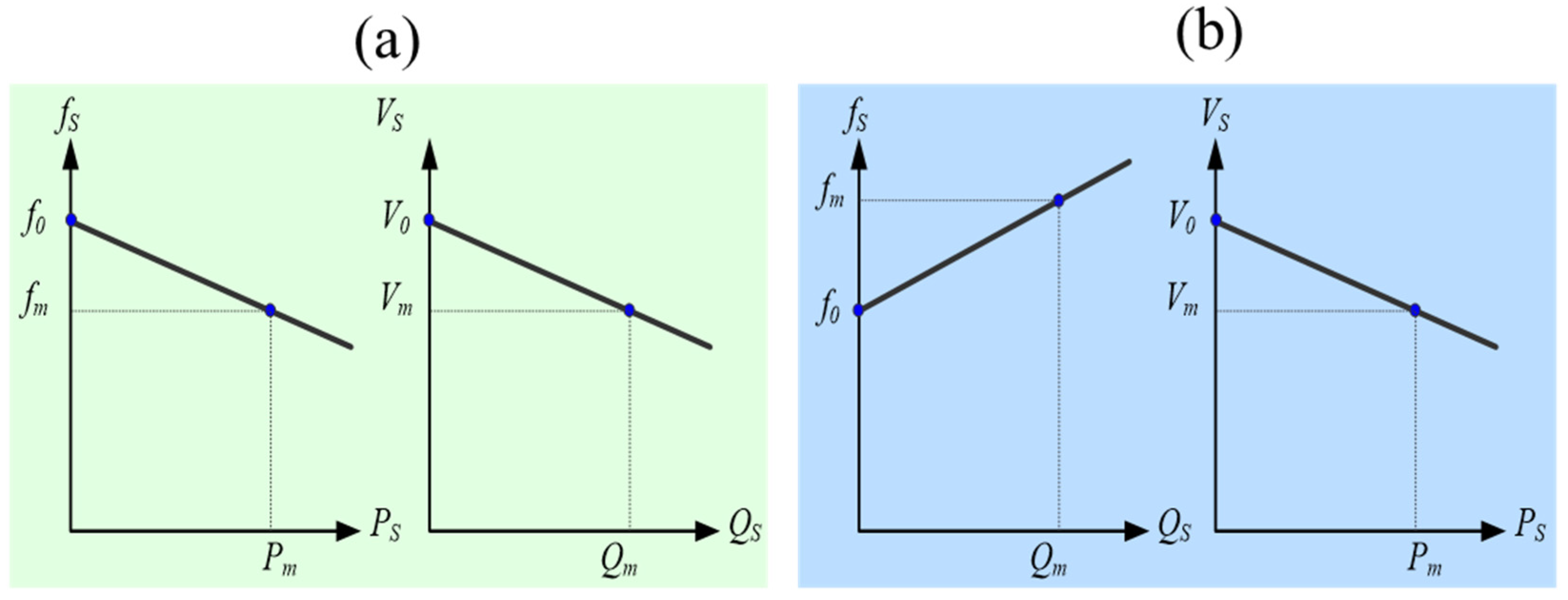
Figure 3 shows plots of both conventional and reverse frequency and voltage droop characteristics. Droop characteristics must ensure that the generated power is distributed evenly throughout various DG units. This is accomplished mostly through an accurate adjustment of the droop characteristics, taking system stability into consideration. In the following section, a variety of essential components required for microgrid design and operation, including the controlling method of each component, are described and modeled. Simulation results are presented and discussed in Section 5.
3. Microgrid Modeling and Design
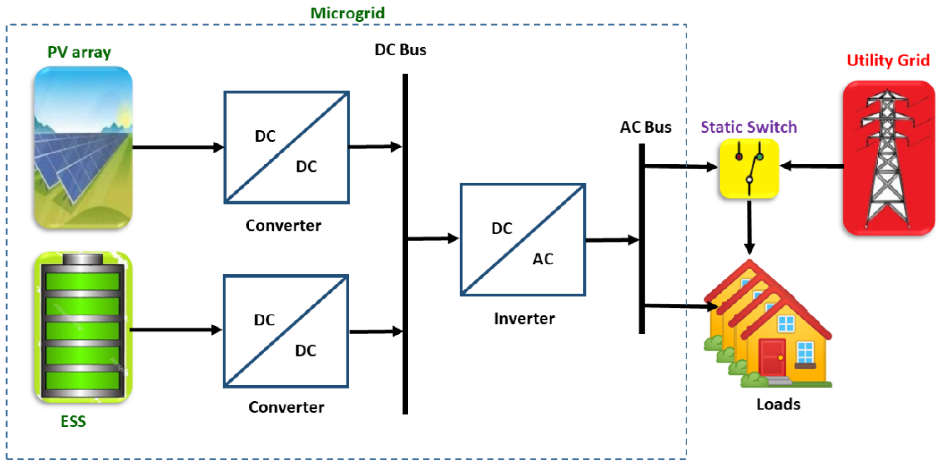
The proposed microgrid architecture includes distributed smart-meters, solid-state transfer switches, circuit breakers, three-phase inverters, PV panels, energy storage system (ESS), DC bus, AC feeders, critical and non-critical loads, and a centralized controller, as illustrated in Figure 4. PV systems are designed to supply all loads within the microgrid coverage area utilizing sizing methodologies in which batteries, PV panel rating, and panel numbers are predicted for the worst-case scenario. The effect on the weather variation on PV panels production was taken into account. The smart power meters, static transfer switches, and microgrid centralized controller are the main components of the proposed microgrid. The controller monitors the power available from the microgrid in addition to that required for the connected loads. If the overall load demand exceeds the microgrid capacity, the controller determines the number and location of loads that need to be transferred to the utility grid. When the microgrid conditions improve and its capacity and voltage attain their nominal values or higher, the transferred load can be restored to the microgrid again.
Detailed modeling and design parameters of the microgrid components were implemented including the PV array, battery array, converters, inverters, solid-state transfer swishes, and microgrid centralized controller. In the following subsections, each component is comprehensively described.
3.1. PV Array
PV Array is typically modeled based on a combination of a number of solar cells connected in series to form a string (NS), in addition to a number of strings connected in parallel (NP) [50]. The building block of the array is the single-diode equivalent circuit of solar cells. The performance of this circuit mainly depends on a five-parameter model including diode ideality factor (n), light-induced current (IL), diode reverse saturation current (Io), series resistance (Rs), and shunt resistance (Rsh). Therefore, the irradiance- and temperature-dependent current-voltage (I-V) characteristics of a solar cell can be computed using the equation [51]:
where K denotes the Boltzmann constant and T is the cell temperature in Kelvin. The PV array current (IPV) and voltage (VPV) with NS series cells/string and NP parallel strings are calculated by [51]:
In this regard, the input model parameters for a 100-kW PV array were set based on a 315 W module (Sun Power; SPR-315E-WHT-D). The module specifications, evaluated at the stranded test conditions (STC), are listed in Table 1. The number of PV modules used to implement this array was set to 320 modules, each module was composed of 96 cells. The modules were arranged in 64 strings; each string consisted of 5 modules. Therefore, in Equation (14), NS is set to be 480 cells/string (96 cells × 5 modules) and NP is 64 strings. The I-V and power-voltage (P-V) characteristics of one module and the whole array, are plotted as shown in Figure 5.
Weather fluctuations have a great impact on the PV panels’ yield. Referring to the power yield measured at the STC, the PV maximum output power (PPVm) is calculated using [52]:
where G represents incoming solar irradiance in W/m2, Pref represents the maximum output power measured by the module manufacture at the STC, λ is a correction factor, and TC represents the temperature in degrees Celsius.
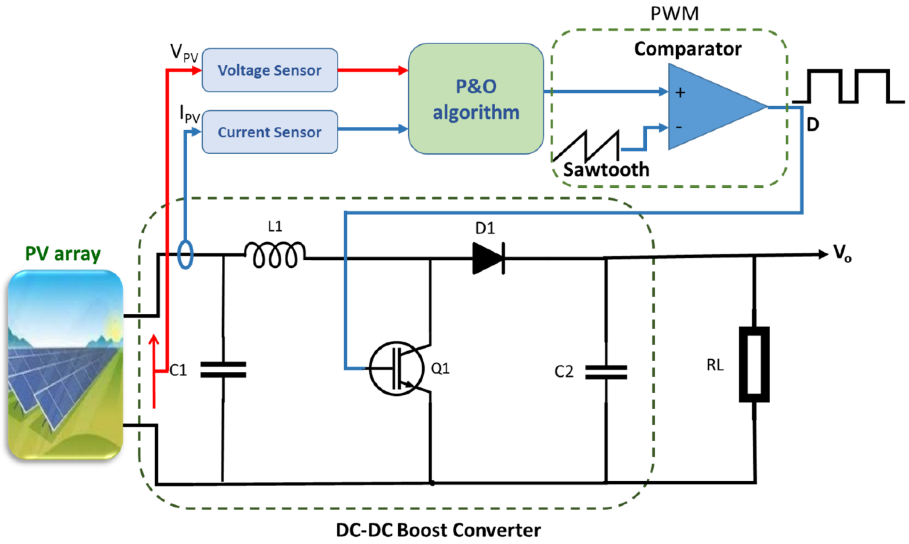
3.2. Boost Converter
To maximize the PV array power yield for variable loads, the DC/DC boost converter controlled by a maximum power point tracking (MPPT) algorithm is generally used. The converter circuit is designed to adjust the operating point always at the maximum power point of the P-V characteristics of the array. As shown in Figure 6, the converter circuit tracks both, the array voltage and current that are typically measured by DC voltage and current sensors. The output of the controller is a duty-cycle ratio (D) that controls the gate of a switching active device (typically it is IGBT). The converter is used to effectively link the PV array to DC-AC inverter(s) and/or to charge a battery array. The extracted PV power using the converter is related to the switch duty-cycle and the load resistance (RL) using the following equation [53]:
Owing to limitations of the switch characteristics, D must be kept within some range (Dmin < D < Dmax). Consequently, the load resistance limits are calculated by [53]:
where Vmpp and Impp are the PV array voltage and current at the MPP. In this design, the duty-cycle ratio was set from 0.1 to 0.9 and the load resistance limits are obtained to be 0.93 to 73.3 Ω, computed at the STC. The converter parameters considered here are listed in Table 2. Regarding the control algorithm of the circuit, the Perturb and Observe (P&O) approach was selected here due to its simplicity, robustness, and small numbers of computed variables required to implement the power tracking process. The P&O tracking method can continuously track the MPP, in different weather conditions, regardless of the kind and location of the PV panels. This is accomplished by analyzing real-time monitoring of PV voltage and current measurements. Because the needed circuitry for implementing MPPTs is more expensive, they are often used for large projects. A pseudocode of the P&O is shown in Algorithm 1. A slight change (perturbation) in the duty-cycle (ΔD) is injected into the circuit throughout the gate of the switch, then PV voltage and current are read (observed) by the sensors. After the change of the power (ΔP) is continuously computed and its sign is checked if it is positive (ΔP > 0) or negative (ΔP < 0), the perturbation continues to increase (Dk + ΔD) or decrease (Dk − ΔD). The performance of the MPPT algorithm is commonly evaluated based on several criteria including (1) time response to rapid and slow variations in irradiance, (2) amount of power fluctuations around the maximum power point and tracking efficiency (TE). The latter parameter can be computed by [54]:
where PPV-average is the average output power of the array that is actually collected by the tracking circuit, and PPV-available is the available power of the array at a certain level of irradiance, which is the maximum power that may be obtained and targeted by the MPPT controller.
| Algorithm 1 Pseudocode of P&O control | |
| 1: | Initialization; Dmin, Dmax, ΔD (duty cycle step), Dk, Vk, Ik, Pk |
| 2: | Read input values of voltage and current Vk+1, Ik+1 |
| 3: | Calculate: Pk+1 = Vk+1 * Ik+1; ΔV = Vk+1 − Vk; ΔP = Pk+1 − Pk; |
| 4: | If ΔP ≠ 0 → If ΔP < 0 → If ΔV < 0 → Dk+1 = Dk − ΔD |
| 5: | else Dk+1 = Dk + ΔD end |
| 6: | else → If ΔV < 0 → Dk+1 = Dk + ΔD |
| 7: | else Dk+1 = Dk +ΔD end |
| 8: | End |
| 9: | else Dk+1 = Dk end |
| 10: | If D ≤ Dmin or D ≥ Dmax → Dk+1 = Dk end |
| 11: | Dk = Dk+1; Vk = Vk+1; Pk = Pk+1; end |
| 12: | Goto step 2 |
3.3. Battery Array and Bidirectional Converter
ESS is essential to compensate for energy shortage and power fluctuations in standalone PV systems. In this design, the battery model was implemented as a controlled voltage source [55].
where V0 is the open-circuit voltage of a battery, AH is battery capacity in Ah unit, k denotes the polarization voltage (V), A is the exponential zone amplitude (V), B is the exponential-zone time-constant inverse (in the unit (Ah)−1), Ibatt is the battery current (A), Ro is the battery internal resistance (Ω), and the integral ∫idt is the charge drawn or supplied to the battery. The state-of-charge (SOC) is a key variable of a rechargeable battery, representing the percentage of the charge level of a battery as compared to its total capacity. Ampere-hour (Ah) counting is a simple and low-complexity method for estimating a battery SOC. To integrate the discharging or charging current and compute the remaining charge in the battery, the Ah counting estimate technique is employed. Therefore, the SOC of a battery is computed as follows [56]:
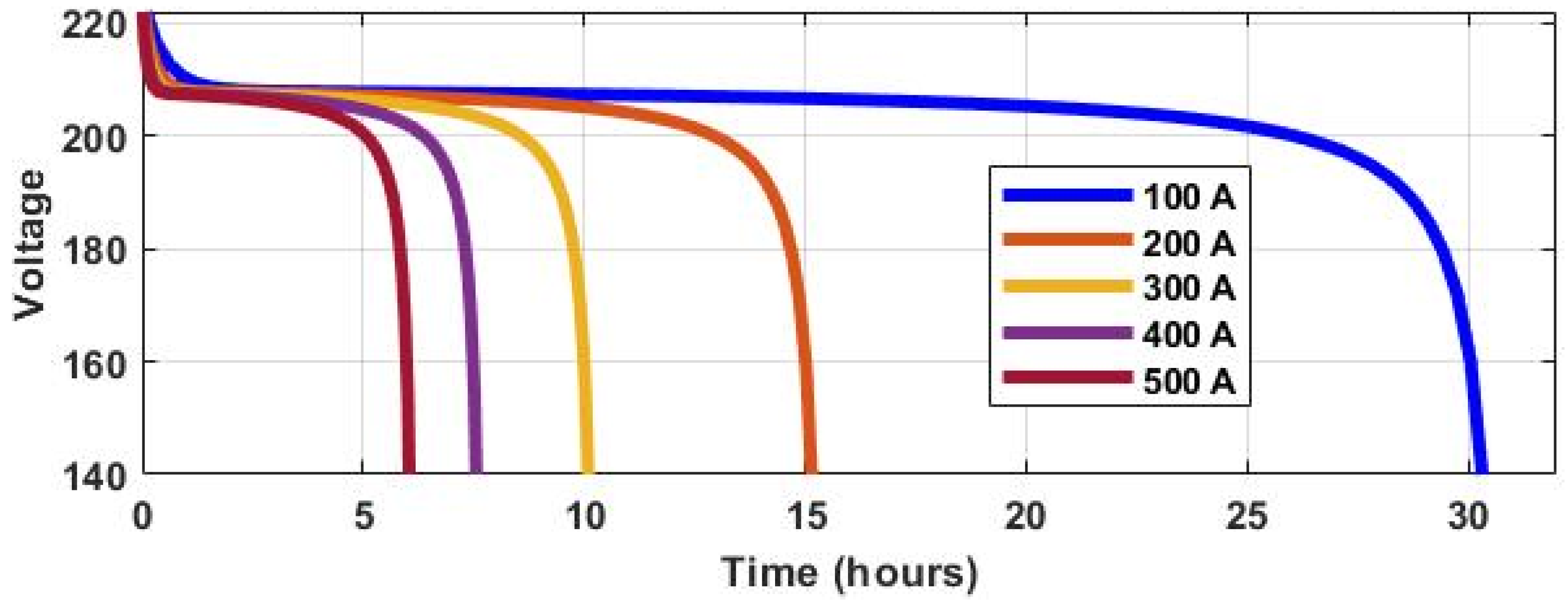
where SOCinit is the initial value of SOC, α represents the usable capacity of the battery. IBatt represents the current which is, by definition, negative during charge and positive during the discharge state. The discharge characteristics of a battery bank with a rated capacity of 3 kAh are illustrated in Figure 7. The typical discharge curve includes three distinguished regions. The first region, at the initial time, represents the exponential decay of the battery voltage when the battery is charged. The second one indicates the battery nominal voltage. The third represents the region at which the voltage drops rapidly, and the battery is discharged.
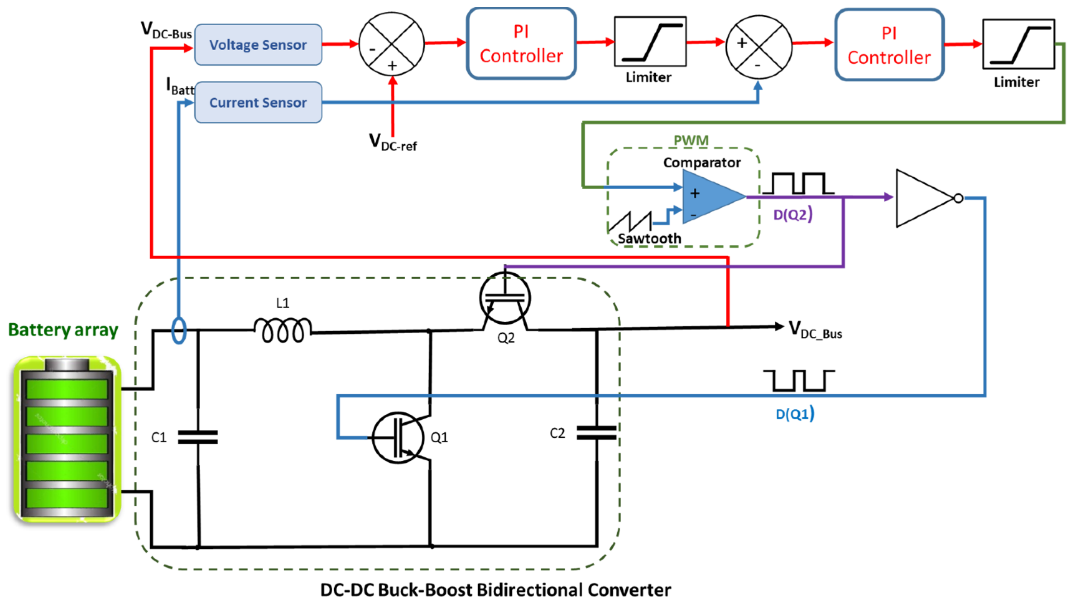
In the present microgrid architecture, the DC bus is linked to the battery array throughout a buck-boost bidirectional converter circuit, as demonstrated in Figure 8. The controller of that converter is responsible for maintaining a regulated DC bus voltage, in addition to charging and discharging the battery array as required [57]. The design parameters of the bidirectional converter are listed in Table 3. The first proportional-integral (PI) controller was used to obtain a constant DC bus voltage (800 V) as compared to the measured bus voltage. The controller parameters were tuned to be kp = 10 and ki = 100 s−1, and the controller output was limited by the maximum charging/discharging current of the battery. The obtained current was used as a reference value and compared with the monitored battery current (IBatt). The error signal was fed to another PI controller to obtain the duty-cycle required to complementary drive the two switching transistors (Q1 and Q2). The parameters of the latter PI controller were optimally tuned at kp = 1 and ki = 10 s−1 with duty-cycle limits of 0.1 and 0.9.
3.4. Three-Phase Inverter
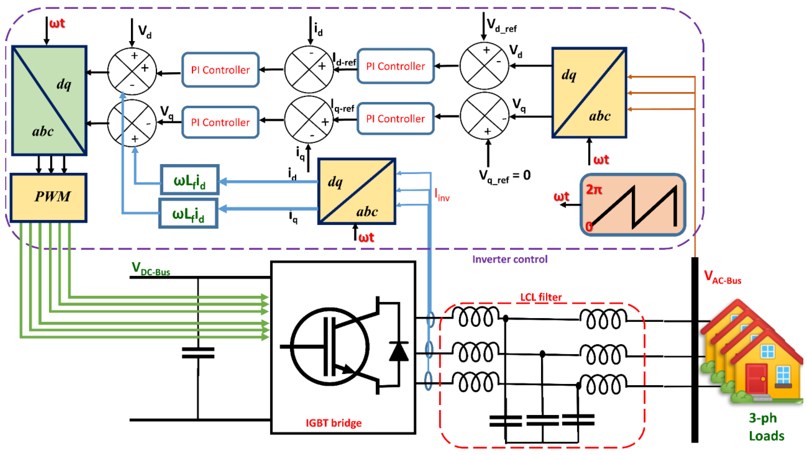
At the load end, a three-phase space-vector controlled voltage source inverter (VSI) serves as a link between the DC-bus and the system loads. The inverter control is utilized to regulate the voltage and frequency at the load side. As the system is not directly connected to the utility grid, the AC-bus voltage amplitude and frequency must be well regulated.
Figure 9 illustrates a schematic representation of the inverter and its control scheme. Generally, a three-phase VSI inverter contains six IGBT power switches in a bridge configuration, interconnected via regulated DC bus voltage through shunt capacitor(s). The inverter harmonic is filtered by an LCL-type filter, which is commonly used in grid-connected and standalone PV systems. The vector control technique is based on a synchronously rotating reference frame. The controller sets the angular velocity (ω) of the rotating axis system, which determines the voltage frequency at the load side [58,59]. The voltage balance across the inductor, Lf in the LCL filter circuit, can be calculated as follows:
where vo a,b,c are output voltages of the inverter, rf and Lf are the resistance and inductance values of the inverter filter, and ia,b,c are the inverter currents. In a rotating direct-quadrate d-q reference frame, the vector representation of a balanced three-phase system and their corresponding vectors can be written as:
If the reverence voltage of the output in the d-axis is set to a constant value vd-ref = |V| representing the required peak voltage at the AC-Bus feeder (|V| = Vrms), and that of the q-axis (vq-ref) is set to zero. Then the inverter active and reactive power can be calculated by:
and
The parameters of voltage PI controllers were tuned at kp = 0.1 and ki = 10 s−1 and those of the current PI controllers were set to kp = 30 and ki = 200 s−1. Table 4 shows the most important design parameters of the inverter.
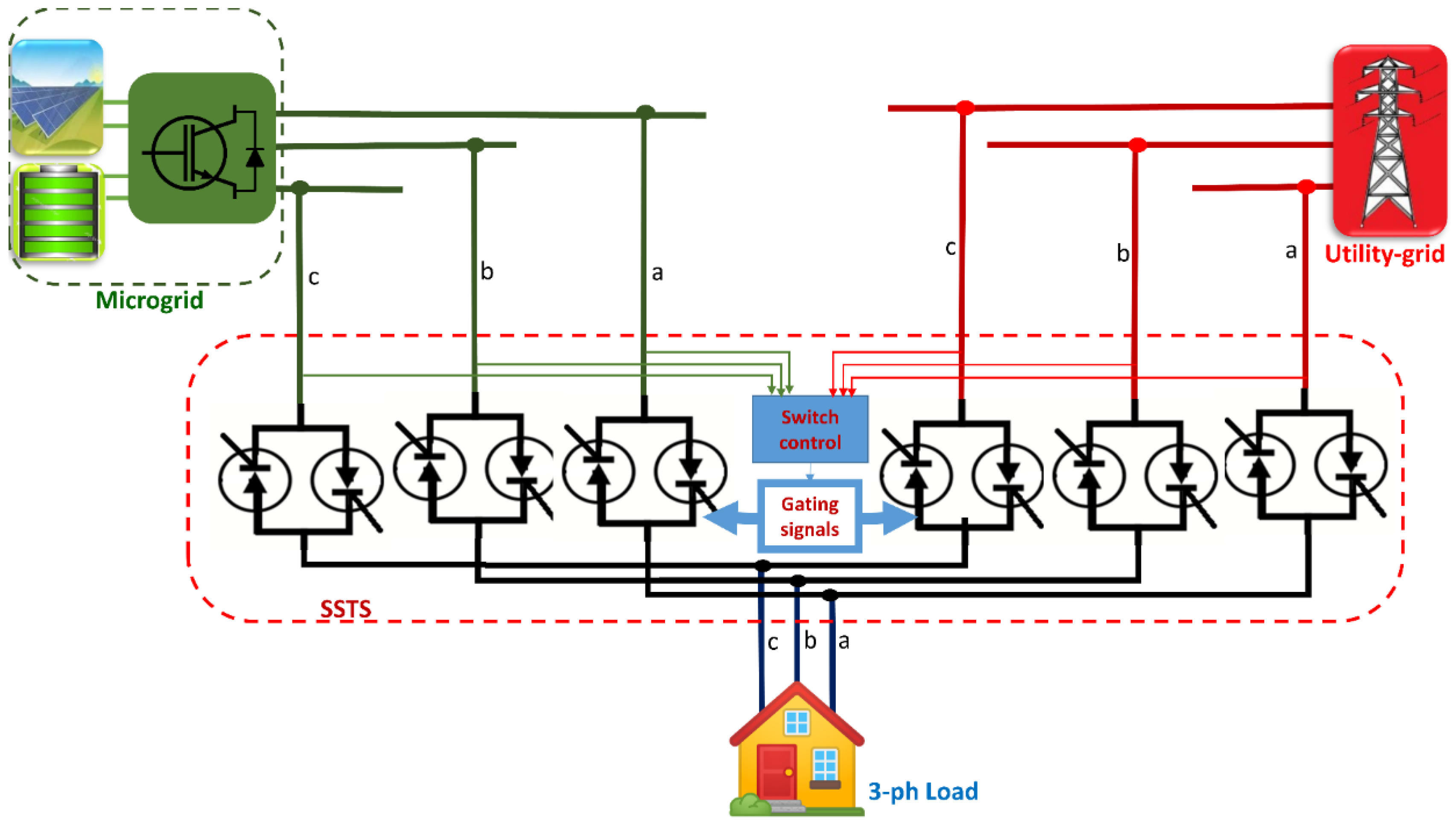
3.5. Solid-State Transfer Switches
Recent research has identified solid-state transfer switches (SSTS) as a potentially cost-effective solution to power control and power quality issues [60]. Figure 10 depicts the basic concept of the SSTS application, to switch selected loads between the microgrid and utility grid. The SSTS commonly contains a pair of thyristor switches for each phase, that assists in power transmission from the primary source, considered here as the microgrid, and the alternative source, considered as the utility-grid, to prevent load power disruptions. The coordinate system is created by instantly transforming the three-phase voltages va,b,c(t) into a bi-axial coordinate system vd,q,0(t). The following equations are used to express the transfer switch operation [60]:
As shown in the above equations, θ(t) is the angle of conversion utilized to determine the amplitude of the vd,q,0(t) vector. The voltage vdq(t) is the continuously monitored voltage that has to be compared to a predetermined threshold voltage in the control algorithm of the microgrid operation. In case the microgrid fails to power the connected loads, a control signal is used to start the transfer process of the assigned loads from the microgrid to the utility grid. Algorithm 2 illustrates the pseudocode used to activate the transfer process by the SSTS.
| Algorithm 2 Pseudocode of SSTS transfer process | |
| 1: | Initialization; threshold voltage of vdq-th |
| 2: | Read actual vdq voltage of the microgrid |
| 3: | Is Vdq ≤ Vdq-min? |
| 4: | If YES → select the loads to be shed from the microgrid → generate transfer |
| signals → transfer the loads | |
| 5: | Goto step 2 |
| 6: | If NO → Goto step 2 |
3.6. Smart Meters
Smart metering aims to provide effective and continuous monitoring of resource usage, and it sends the collected data to the Internet or local server through IoT technology. Smart meters are the most common name for these metering devices. While there is a wide range of devices on the market today, the most difficult part is integrating them into a useful smart metering solution for a specific application. The IoT-based smart meter should be able to accommodate all smart meter features in near real-time in addition to guaranteeing two-way communication with a sample rate of roughly 1 s. In residential load demand settings, two types of electric loads are commonly used: linear and non-linear loads. The present design of the smart meter accounts only for monitoring residential linear loads (lighting, refrigerator, air conditioner, fan, heater, etc.). The expressions for voltage and current in the AC time domain can be represented by the following equations:
and
where Vm denotes the maximum voltage amplitude and ω denotes the voltage’s angular frequency, which should be fixed by the utility provider. Im is the current amplitude, and θ is the phase angle between the voltage and current. The apparent power (S) can be calculated using the root-mean square (rms) values of the voltage and current as follows:
The rms values of the current and voltage can be estimated after the instantaneous values of the current and voltage have been collected, using discretization techniques:
where N denotes the sample size of the discrete voltage and current values vn and in, respectively. On the other hand, the real power (P) is simply the average value of the multiplied discrete values of the voltage and current:
Therefore, the power factor (PF) is obtained by:
The reactive power (Q) is calculated by:
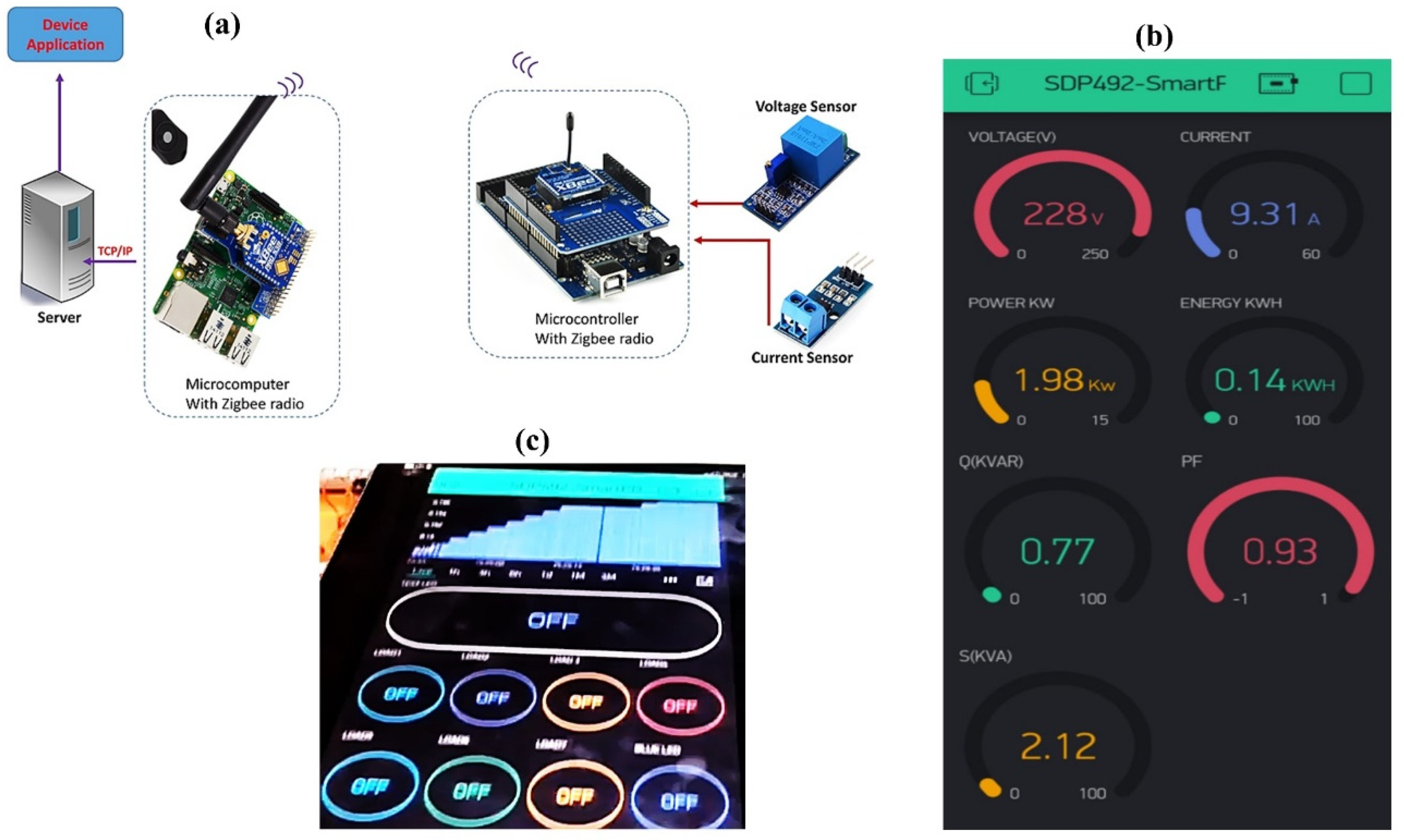
Figure 11a illustrates the prototype design of the smart meter, which was implemented using ZMPT101B voltage sensor and ACS712-30A current sensor. Microcontroller (ATmega328) and microcomputer (Raspberry Pi 3 model B) devices each equipped with XBEE-S1C module, using ZigBee communication protocol, were set up to transmit the measured data to an IoT server. The Raspberry Pi 3 model B was chosen here because of its features, which include a quad-core 64-bit ARM Cortex-A53 clocked at 1.2 GHz along with 1 GB RAM. Moreover, it is equipped with graphics capabilities provided by its GPU VideoCore IV. Regarding its compact size, ease of configuration, low cost, high speed, and low power consumption, which makes it is suitable for many IoT applications and prototyping. More recently, Pi 4 model with 8 GB RAM is also available with improved capability and reliability. The metering data were saved and pre-processed at the edge before being uploaded to an application operating on a cloud middleware platform (Blynk IoT). The platform has all the needed functions to remotely manage IoT devices such as provisioning, over-the-air firmware update, secure data storage, data analytics, and visualization. Blynk supports many hardware devices including Arduino and Raspberry Pi. We used the Blynk mobile application to display the manipulated data for consumer load profiling, energy demand, and appliance remote control in the dashboard shown in Figure 11b. The data collected by the meter are represented by 10-bit accuracy and sent a reading every 1 s. The results of measuring and assessing the data transmission bit rate of the designed smart meter are displayed and discussed in Section 5.
3.7. Microgrid Control
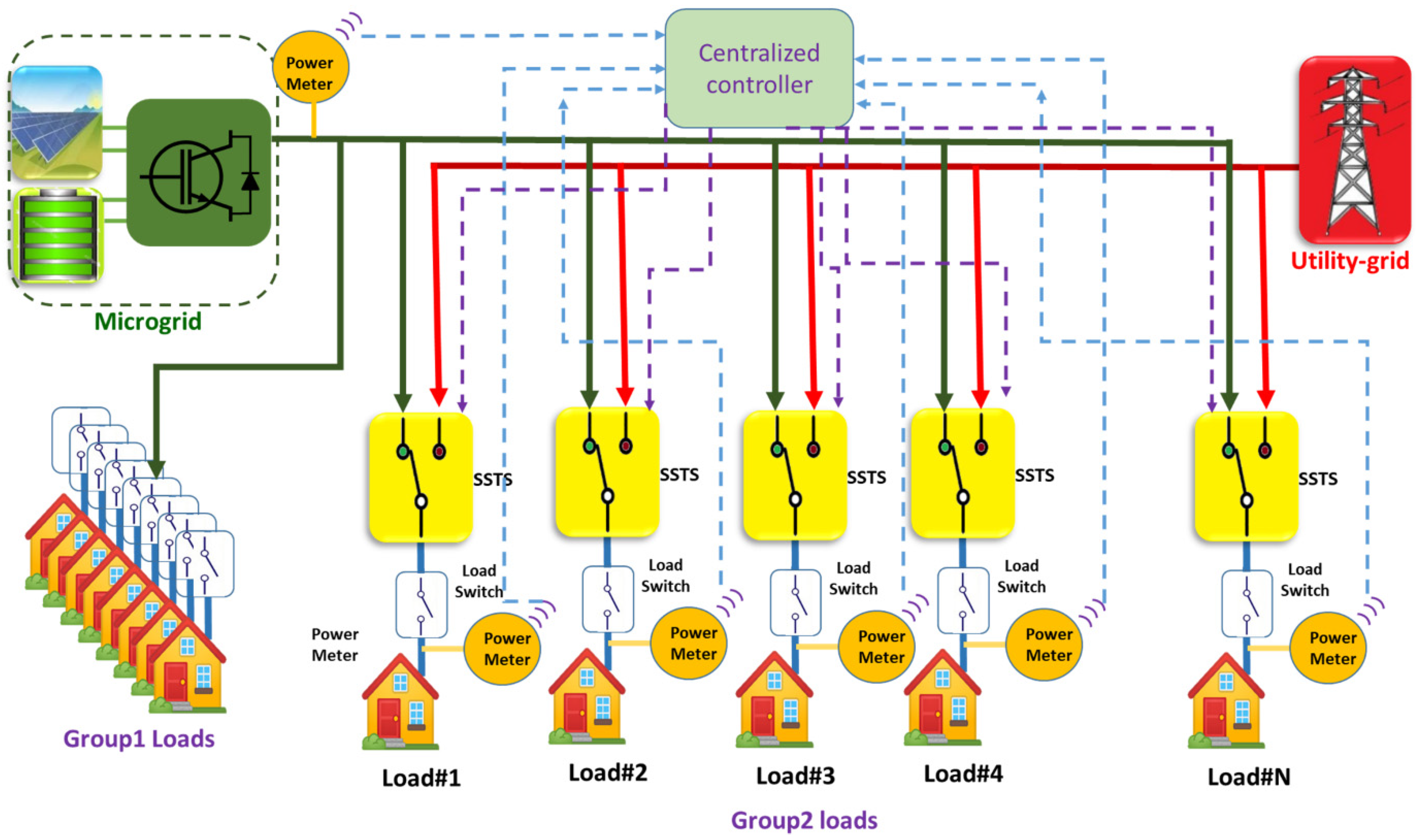
Figure 12 demonstrates the detailed architecture of the PV-ESS microgrid equipped with a centralized controller used for power management. The connected loads are classified into two groups: group1 includes the high priority loads that must be permanently connected to the microgrid, while the other group includes fewer priority loads that can be islanded from the microgrid and reconnected to the utility grid through SSTS. The controller runs an algorithm that requires a set of consents and variables such as: number of loads (N), the threshold voltage (VµG-min = vdq-min) that can be extracted from voltage-power characteristics (V-P) of the microgrid, the real-time monitored microgrid voltage at the AC-bus (VµG), and a power margin (ΔP) used to adjust the amount of load shedding, as described in Algorithm 3. At regular intervals, the algorithm checks the power demands (PD) and compares them with the power produced by the renewable resources (PDER). If the demands exceed the microgrid capacity and the microgrid voltage falls below the predetermined threshold voltage, the algorithm classifies the loads and calculates the number and location of loads that must be removed from the microgrid. Upon receiving the transfer signal from the microgrid controller, the selected loads are momentary and seamlessly transferred to the utility grid. The LoRa communication network is used to communicate between the transfer switches, power smart-meters, and grid controllers. When the operating conditions of the microgrid get improved or the demand is reduced, the transferred load(s) can be restored to the microgrid.
| Algorithm 3 Pseudocode of loads selecting and transferring to the utility-grid | |
| 1: | Initialization N, VµG-min, VuG–nominal, ΔP |
| 2: | Read VµG, PDER, [PL1,PL2,…PLi,..,PLN] |
| 3: | Calculate present power demand PD ← |
| 4: | If VµG ≤ VuG–min then |
| 5: | Calculate Pdiff = PD − PDER + ΔP |
| 6: | Find the load m such that PLm is the nearest value to Pdiff |
| 7: | Disconnect Load m from the microgrid and transfer it to the utility-grid |
| 8: | Else if VµG > VuG–nominal then |
| 9: | Restore the Load m to microgrid |
| 10: | Else Return |
4. Design of the IoT Communication Network
IoT technologies offer three classes of communication standards: PAN (Personnel Area Network), LAN (Local Area Network), and WAN (Wide Area Network). For instance, compared with Wi-Fi technology, the ZigBee communication protocol is very effective in creating a home area network (HAN). The communication link between smart meters and the centralized controller can be assured by wireless or wireline WAN/LAN communication protocol. The classifications and comparisons among these protocols have been discussed in [61]. The LoRa communication protocol is a very attractive solution for building private, secure, and low-power communication infrastructure for microgrids [62,63]. LoRa uses spread spectrum technology which employs a low-complicity receiver, making it a suitable choice for machine-to-machine (M2M) communication, IoT, wireless sensor networks, and many other applications. Nodes in a LoRaWAN network are not linked to a single gateway. Therefore, data sent by a node are usually received via a number of gateways. Through some downlink, each gateway will transfer the received data from the end-node to the cloud-based network server. That server could be Wi-Fi, Ethernet, cellular, or satellite-based network. The server handles the complexity and intelligence required to administrate the network, filtering redundant incoming data packets, doing security checks, scheduling acknowledgments through an optimized gateway, and performing adaptive data rate, among other things. The nodes in a LoRaWAN network are asynchronous, which means that they communicate to each other only when they have data to be broadcasted, whether the data transfer is scheduled or event-driven. This technique can greatly save the energy required to operate LoRaWAN devices (i.e., increase battery lifetime).
The incorporation of security into any low-power wide-area network (LPWAN) is critical. LoRaWAN has two security layers: one for the application and another for the network. The security application layer guarantees that the network operator does not have access to the end-user application data, while network security assures that each node in the network is legitimate. The key exchange is encrypted using an advanced encryption standard (AES) and an IEEE EUI64 identifier. Because of regional spectrum allocations and regulatory restrictions, the LoRaWAN specifications differ somewhat from region to region.
End-node devices are used for different purposes and have varying requests. LoRaWAN uses multiple device classes to optimize a range of end-node device applications. The device classes compromise network downlink communication latency versus battery life. In many applications, communication latency is a crucial element in any actuator-type or control-type application. The latency requirements for implementing the DR program have been studied in research and industrial trends [62,63,64]. However, in the context of smart grids, there have been limited efforts devoted to using them in isolated-mode microgrids. The features of LoRa are summarized in Table 5.
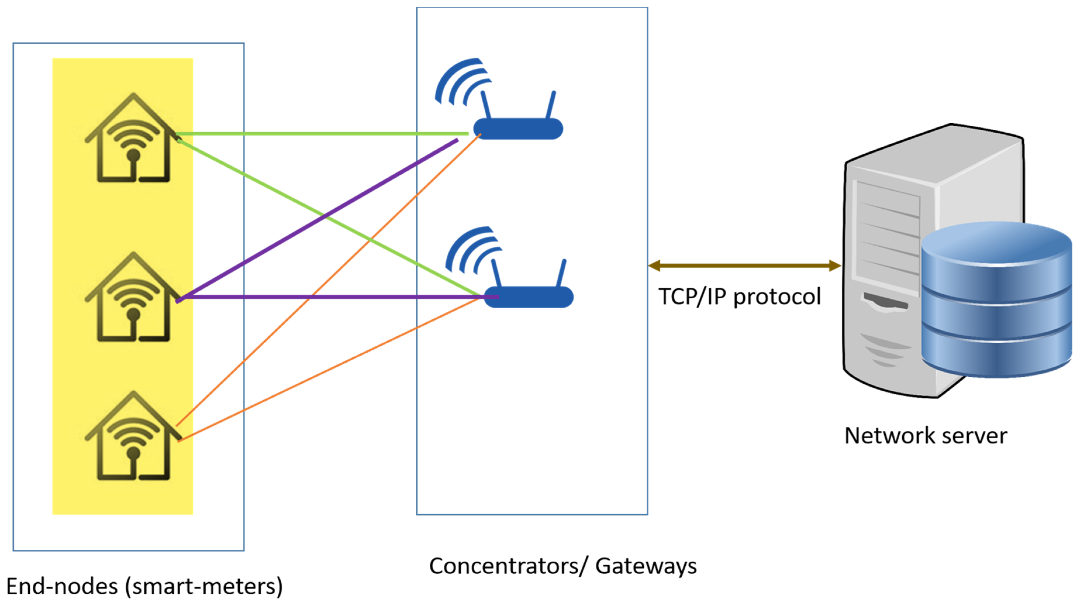
LoRa supports three classes of devices A, B, and C, as listed in Table 6. Each uplink end-device data transmission is followed by two short downlink reception windows, allowing for bi-directional communications. The end-transmission interval is determined by its own communication requirements, with a slight variance depending on a randomized time basis. In LoRa, class A device consumes low energy, most of the time in sleeping mode, transmits data to the gateway. These devices are used mainly to design battery-operated IoT sensor nodes. Bidirectional communication between a LoRa class A device and a gateway is supported. At any moment, uplink communications (from the device to the gateway) can be initiated. After an uplink transmission, the device opens two receive windows at predetermined periods. If the gateway server does not answer in any of these receive windows, the device’s next opportunity will be after the next uplink transmission. In Class B devices, additional receive windows are open at predetermined time intervals. The end-device gets a time-synchronized signal from the gateway in order to open its receive window at the predetermined time. This informs the server about the end-listening device status. Class C devices always have open receive windows and only close when they are in the data sending mode. Figure 13 shows the architecture of the LoRaWAN network.
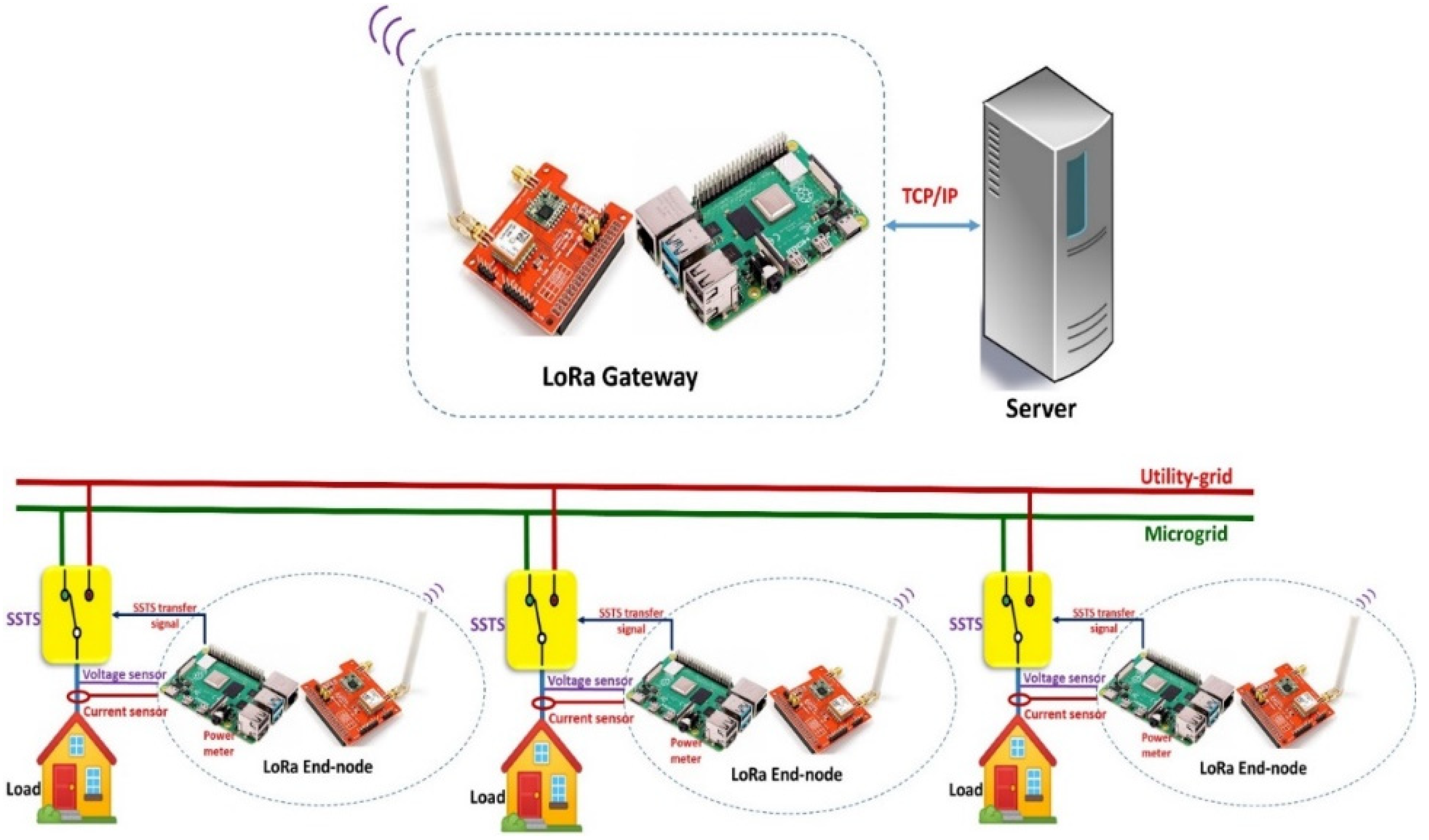
The smart meters in our proposed microgrid architecture can be implemented using LoRa end-node class B or class C devices. Figure 14 illustrates a representation of IoT LoRa-based communication network within the proposed microgrid design. In this context, low-cost microcomputers, such as the Raspberry Pi devices, can be used to implement the end-nodes, gateways, and the centralized controller. The smart meter features continuous monitoring to load power in addition to microgrid bus voltage. Management of the battery bank and its SOC can be also taken into consideration. A Raspberry Pi-compatible LoRa shield is used to construct the LoRaWAN-based fog computing, while the gateways can be designed using LoRa GPS HAT along with Raspberry Pi devices. The gateways directly communicate to the network server using TCP/IP protocol. The microcontroller LoRaWAN gateway collects the incoming data from smart meters and sends it to the TCP/IP server for further processing. The load power is calculated based on collected data from accurate voltage and current sensors. At the same time, the SSTS transfer signals are generated by the end-node devices based on event-based control signal directed from the network server. The smart meter operates as a LoRaWAN node, collecting data from smart controllers and charge controller agents and sending it through LoRaWAN. Using the LoRaWAN class B node and LoRaWAN gateway, the results showed that a latency of within 1 s is attainable. The power meter at the load side (prosumer) of the microgrid, sends the microgrid voltage and load power data every second. The required latency is then below 1 s and the payload is 1000 bytes.
The physical layer of LoRa network mainly depends on the chirp spread spectrum (CSS) transmission technique, which can achieve both low power and long-range communication. In addition, the modulation in LoRa devices is highly adaptable and can be configured to provide data at speeds of up to 50 kbps. On the other hand, the un-optimized settings of operation can lead the data transmission rate to be extremely low. Therefore, customizable settings define the LoRaWAN characteristics and performance. The key parameters that greatly affect LoRa network performance, especially the data transmission rate are: operating frequency, bandwidth, spreading factor, and correction rate. Regarding the modulation frequencies, LoRa communicates over license-free radio frequency bands that differ from one region to another. For example, in North America, the 915 MHz frequency is used, while in Europe it is 868 MHz, and in Asia the 169 MHz, 433 MHz are used. The bandwidth (BW) determines the range of frequencies that coded information is spread within. Higher BW gives a faster data transmission rate however it increases noise sensitivity. In LoRa, the BW sets are typically 125, 250, and 500 kHz. Spreading Factor (SF) is the proportion of the symbol rate to the chip rate, and commonly takes a value of between 7 to 12. A higher SF increases the signal-to-noise ratio, transmission range (to be in the km range), and Time-On-Air (TOA) of a data packet. The coding rate CR can take the following values: 4/5, 2/3, 4/7, and 1/2. Increasing CR would increase data transmission rate; however, this can reduce the TOA, and therefore, data transfer becomes less reliable. Based on the above-mentioned parameters, the transmission rate (Rb) in bps for the LoRa network is given by:
In the following section, a suitable configuration setting of a LoRa-based communication network that fulfills efficient communication link within the microgrid is to be discussed.
5. Results and Discussion
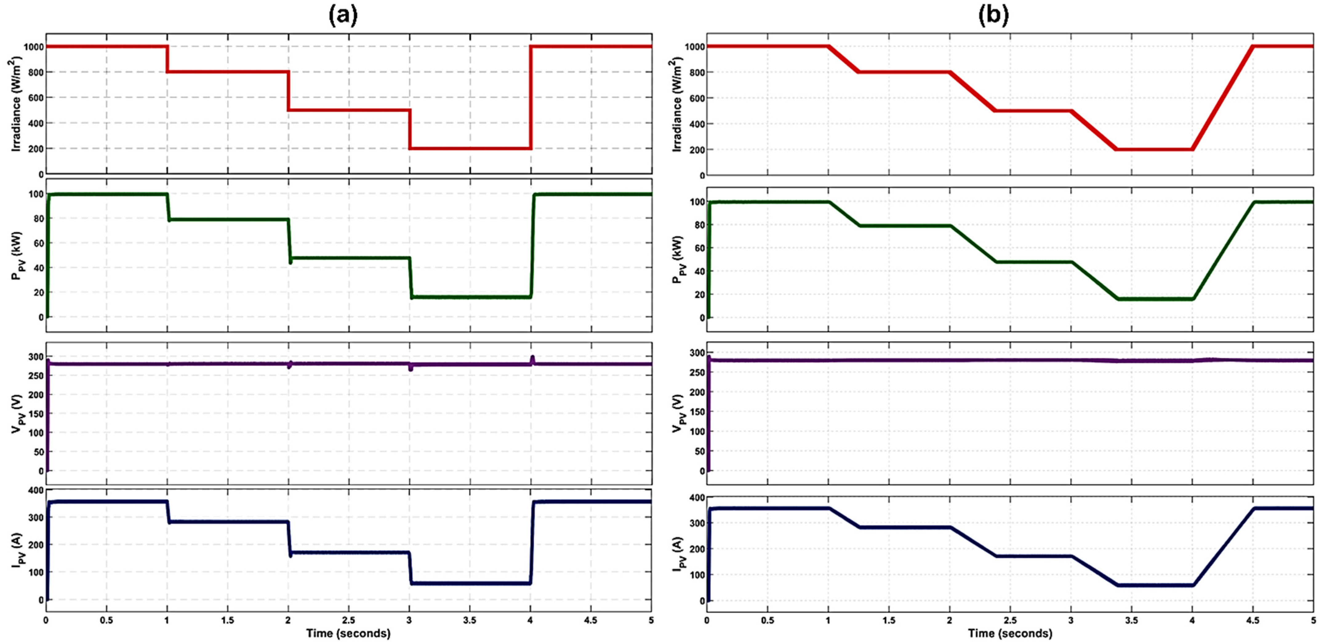
We used Matlab/Simulink software 2020a edition, equipped with a powerful toolbox for designing and simulating microgrid components utilizing specialized power systems libraries. In this section, we explore the most important results of the above-mentioned microgrid design, starting with the PV array and its power tracking unit. The MPPT circuit is tested in both conditions: the transient and steady-state change in the irradiance. The simulated PV output power (PPV), voltage (VPV), and current (IPV) waveforms are shown in Figure 15a. The system performance was initially tested at a sudden reduction in the solar irradiance from 1000 to 200 W/m2 in three steps and then suddenly raised from 200 to 1000 W/m2 in one step. The results show that the designed tracking circuit exhibits a high tracking efficiency, TE, that reached 99.5% at PPV = 100 kW in addition to a fast response that is less than 25 ms to reach the steady-state conditions. At these abrupt changes in the irradiance, the simulation results proved that the system achieved minimal fluctuations in tracked PPV that is less than 4% in the worst case. Moreover, regardless of the irradiance level, the output power fluctuations are mostly eliminated at the steady-state operating point. In most applications, the progressive increase or decrease of irradiation is the practical condition. Therefore, the tracking performance of the designed MPPT circuit was also tested for gradual change in the irradiance as shown in Figure 15b. The irradiance was gradually reduced from 1000 to 200 W/m2 and then increased from 200 to 1000 W/m2 with raising and falling rates of +1600 and 800 W/m2/s, respectively. As a result, the designed controller clearly accomplished the slow variations of the irradiance with a considerable tracking accuracy in a short period of time, of less than 25 ms, with a minimal fluctuated power, that is less than 2.5% in the worst case.
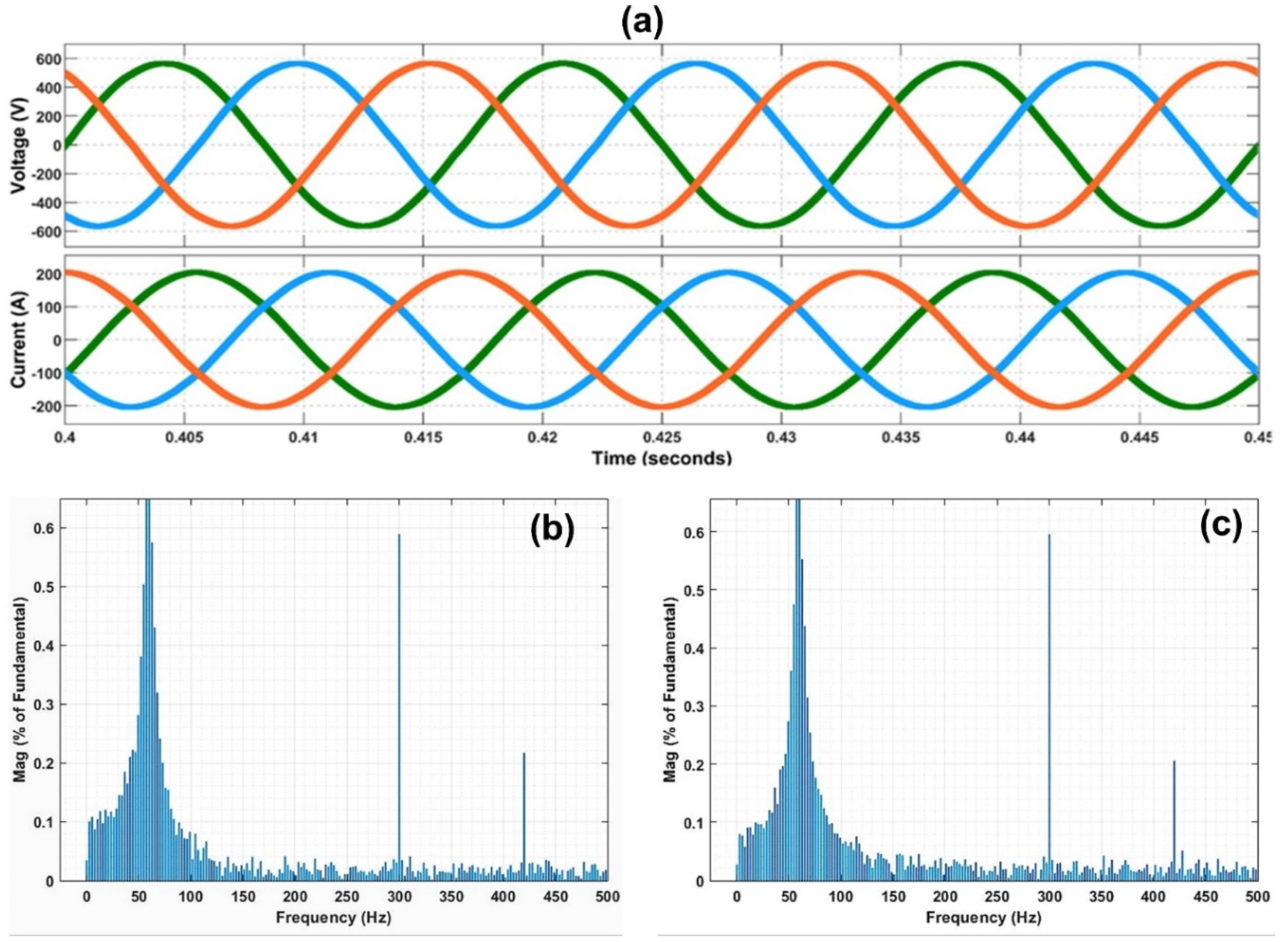
Owing to using many power electronic switches in the power conditioning units within the microgrid, harmonic distortion commonly occurs. The total harmonic distortion (THD) is a critical issue in power systems, especially microgrids operating in islanded and partially grid-connected modes. Therefore, THD must be kept to a minimum to be less than 5% in order to meet the standards. Reduced THD in microgrids results in a greater power factor and lower electricity expenditures, resulting in improved power conversion efficiency. It is worth it here to figure out how much harmonic distortion is present in the designed system. Figure 16 depicts waveforms of instantaneous voltage and current of the AC-bus of an islanded microgrid at a load power of 100 kW. The waveforms indicate nearly pure sinusoidal with low harmonic distortion. The FFT analyzer was used to do the THD analysis, as depicted in Figure 16b,c. The analysis revealed that the THD of the voltage and current waveforms were computed to be 1.24% and 1.27%, respectively. This implies the good performance of the inverter controller and its related design parameters.
Figure 17a depicts the variation of PV power, SOC, and battery power when changing of load power computed at different irradiance levels. At higher irradiance levels (1000 W/m2) and lower power consumption by the loads, PV power is maximized to 100 kW, while the battery power is negative indicating the charging state of the batteries. When the load power increases and at the same time the irradiance level decreases, the power delivered from the PV array is reduced and compensated by the batteries. At a very low irradiance level and full load, most of the power is delivered from the batteries and its state is mainly discharging. The main objective of the battery in this system is to supply critical loads during the night and temporarily support the load demand during cloud trainsets which usually take a few minutes.
In the case of the persistence of clouds for long periods or during the night, the demand is partially supplied by the battery bank and the non-critical loads are switched to the utility grid. To study this case, a load profile of an academic institute is adopted [65]. The critical load is chosen to be 20% of the peak power (20 kW) of the load demand. With a total absence of irradiance for one day, a suitable size of the battery is calculated to be 480 kWh. If the SOC of the battery is nearly fully charged (95%) and under the assumption of the total absence of irradiance in the next day, the battery power should be increased up to 600 kWh. Therefore, the battery bank with this rated capacity is capable to provide power to the critical loads for 24 h, as shown in Figure 17b. The above case represents the most extreme conditions to operate the system. However, for weather conditions, like in Saudi Arabia which has a clear sky condition for most of the year, the battery bank is sized to supply the critical loads at the night and during short cloud periods during the day. This means the suitable size of the battery for the above-mentioned case can be reduced to be in the range of 240 kWh.
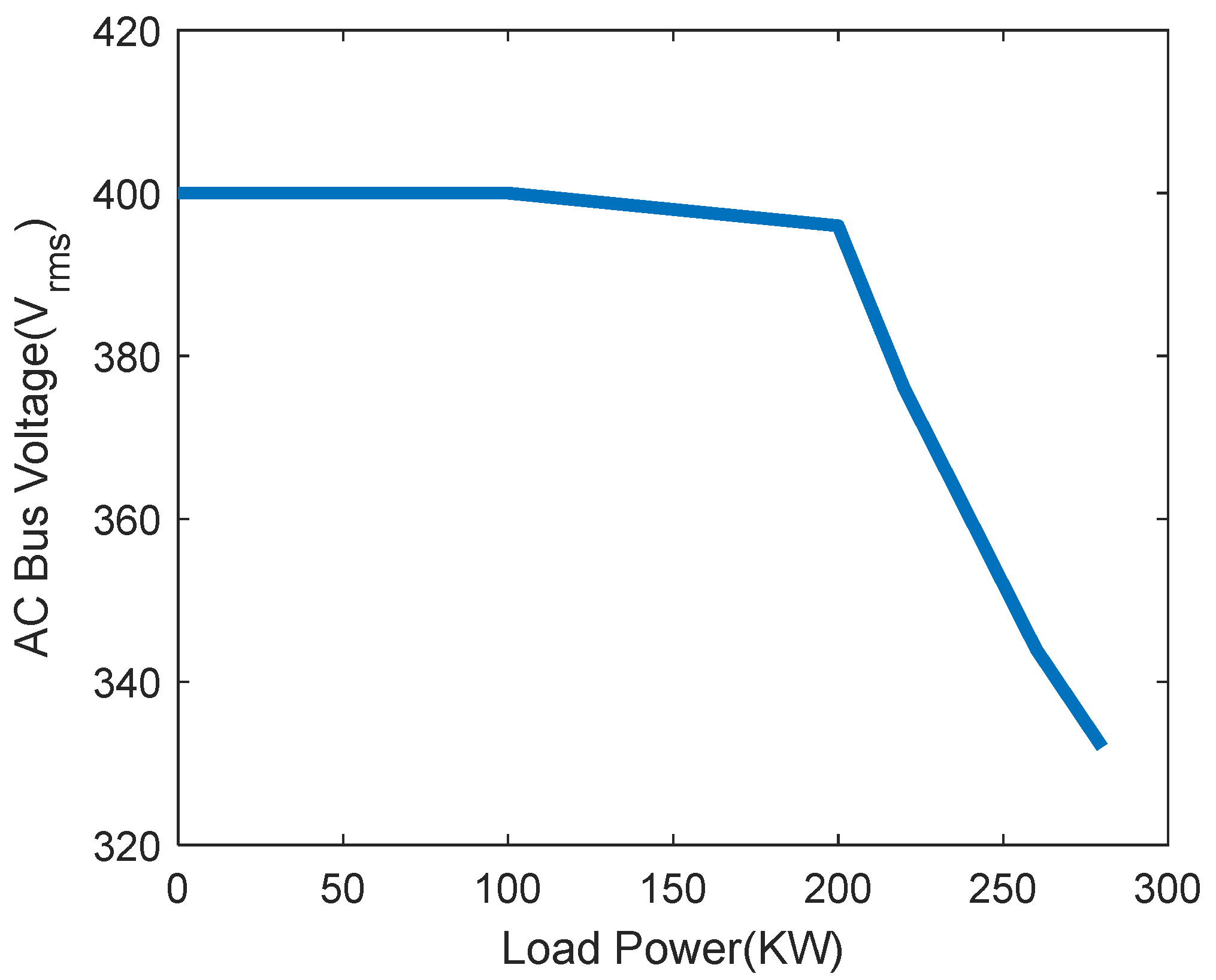
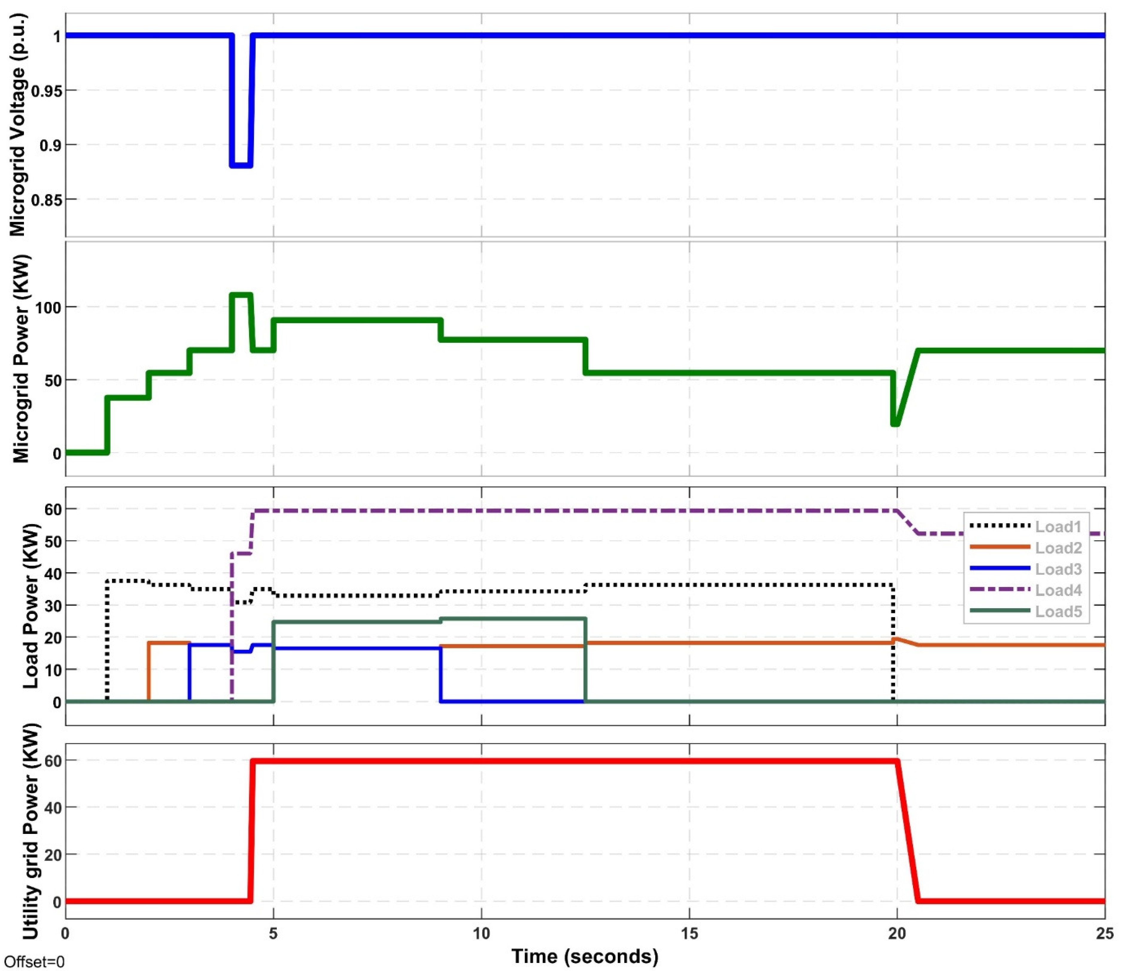
Figure 18 displays voltage power curve of the microgrid in which the voltage regulation action of the controllers is clearly achieved. The controllers succeeded in regulating the voltage to be within 10% of its nominal value for load power change up to 200 kW. After this limit, a load shedding action should be taken to prevent the unstable operation of the microgrid. However, instead of load shedding, some loads are carefully selected to be transferred to the utility grid in the partially grid-connected mode. The selection procedure is achieved by the above-mentioned algorithm. An example to verify the proposed algorithm result is displayed in Figure 19. In this case, the algorithm is applied on five non-critical loads of 40, 20, 20, 60, 25 kW. The loads are sequentially connected to the microgrid at times of 1, 2, 3, 4, and 5 s, respectively. As displayed in the figure, the connection of load#4 resulted in a significant voltage drop below the accepted limits (10% of the nominal voltage). In this situation, one or more loads have to be disconnected from the microgrid and transferred to the utility grid. The selection of this (or these) load (s) depends on the power difference between the load demand and the available power of the microgrid. In this case, load# 4 was selected to be transferred to the utility. When the load demand decreases or the microgrid conditions were improved, the voltage attained its nominal value, therefore the disconnected load was restored to the microgrid again.
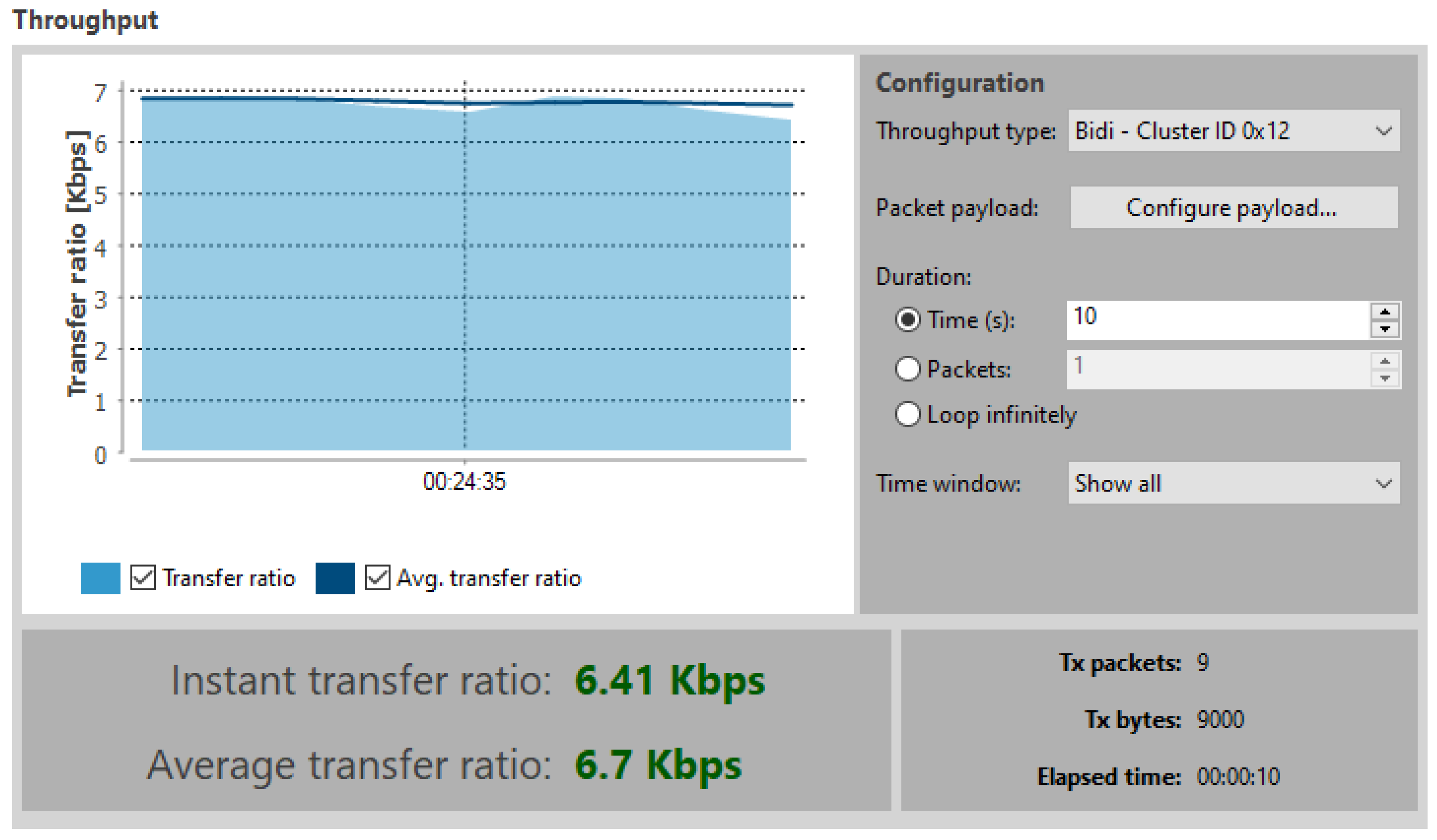
Regarding the IoT network, the designed smart-meter prototype was evaluated from the data transmission point of view. The measured data throughout boosted mode communication is depicted in Figure 20. The measured results show that ZigBee with a bit rate of 6.7 kbps is capable of handling the bit rate and latency required for effective reporting of the load demands to the microgrid controller through the designed IoT connection. The latency for the communication between the smart meter and the controller in this measurement was within 10 s. To assess the effectiveness of the LoRa communication protocol in handling the communication requirements (bitrate, latency, and coverage) between smart meters and the microgrid controller, the LoRa physical layer was simulated using Matlab. The smart-meter has been modeled using LoRa class B, whereas the microgrid controller has been modeled as a class C device.
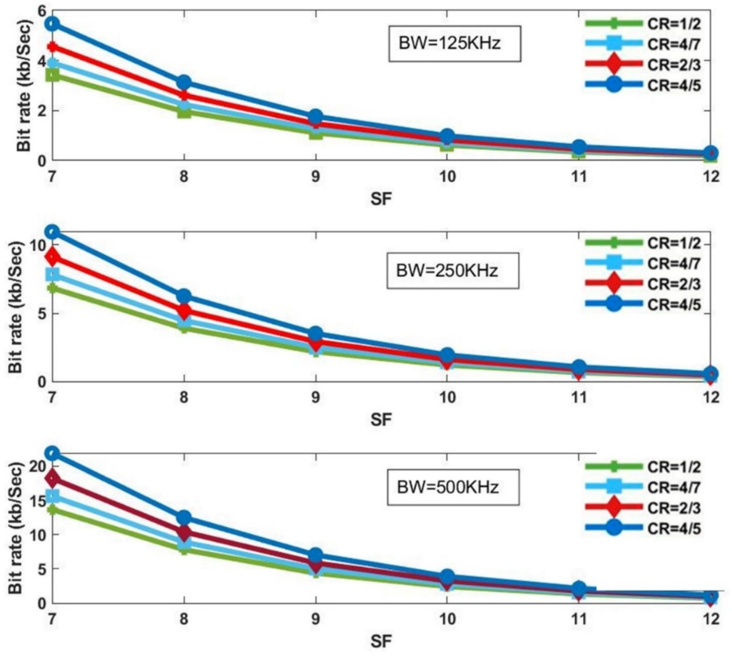
Figure 21 displays bit rate versus SF of LoRa physical layer in which different configurations can be customized for end-node and gateway LoRa devices. In a microgrid, loads do not change very often, therefore microgrid voltage and power, in addition to load power, are monitored by smart meters and sent to the gateway at a sampling rate of 600 samples per second. The data are collected by voltage and current sensors, then converted into digital samples using an analog-to-digital (ADC) converter of 10-bit accuracy, which makes the data bit-rate equal to 6 kbps. Taking into account the communication overheads, a LoRa device should offer a bit rate of 8 kbps. Accordingly, LoRa parameters can be configured as follows: carrier frequency of 433 MHz, BW of 250 kHz, SF of 7, and CR of 2/3.
6. Conclusions
This paper provides a proposed design and control method for a partially grid-connected PV microgrid. The control and architecture are designed to connect or detach non-critical loads between the microgrid and the utility grid. PV arrays, energy storage elements, inverters, solid-state transfer switches, smart-meter, and communication network of the microgrid were modeled, designed, and simulated using the Matlab/Simulink software. The LoRa communication network was used to design the IoT-based communication system between the smart meters and the microgrid controller. An IoT-enabled smart-meter with ZigBee connectivity has been built for comparison with the proposed LoRa end-node communication protocol requirements. For microgrid applications, appropriate configurations of LoRa physical layer devices were suggested to be with a bandwidth of 250 kHz, spreading factor of 7, and correction rate of 2/3.
7. Future Work
We intend to implement the design proposed here in a down-scale experimental model. The main focus is to test the performance of the proposed system under different communication system requirements and configurations for microgrid applications.
Author Contributions
Conceptualization, M.S., and I.B.D.; methodology, M.S.; software, M.S.; validation, I.B.D. and M.A.-A.; formal analysis, M.S. and M.A.-A.; investigation, M.S. and M.A.-A.; resources, M.F.A.; data curation, I.B.D. and M.A.-A.; writing—original draft preparation, M.S.; writing—review and editing, M.S., I.B.D., M.A.-A. and M.F.A.; visualization, M.S.; supervision, M.A.-A. and M.F.A.; project administration, M.F.A. All authors have read and agreed to the published version of the manuscript.
Funding
This research received no external funding.
Institutional Review Board Statement
Not applicable.
Informed Consent Statement
Not applicable.
Acknowledgments
The authors would like to thank the Deanship of Scientific Research, Qassim University for funding the publication of this study.
Conflicts of Interest
The authors declare no conflict of interest.
References
- Moghaddam, A.A.; Seifi, A. A comprehensive study on future smart grids: Definitions, strategies and recommendations. J. N. Carol. Acad. Sci. 2011, 127, 28–34. [Google Scholar] [CrossRef]
- Almohaimeed, S.A.; Abdel-Akher, M. Power Quality Issues and Mitigation for Electric Grids with Wind Power Penetration. Appl. Sci. 2020, 10, 8852. [Google Scholar] [CrossRef]
- Selim, A.; Abdel-Akher, M.; Kamel, S.; Jurado, F.; Almohaimeed, S.A. Electric Vehicles Charging Management for Real-Time Pricing Considering the Preferences of Individual Vehicles. Appl. Sci. 2021, 11, 6632. [Google Scholar] [CrossRef]
- Kharrich, M.; Kamel, S.; Ellaia, R.; Akherraz, M.; Alghamdi, A.; Abdel-Akher, M.; Eid, A.; Mosaad, M. Economic and Ecological Design of Hybrid Renewable Energy Systems Based on a Developed IWO/BSA Algorithm. Electronics 2021, 10, 687. [Google Scholar] [CrossRef]
- Fang, X.; Misra, S.; Xue, G.; Yang, D. Smart grid—The new and improved power grid: A survey. IEEE Commun. Surv. Tutor. 2011, 14, 944–980. [Google Scholar] [CrossRef]
- Gellings, C.W. The Smart Grid: Enabling Energy Efficiency and Demand Response; CRC Press: Boca Raton, FL, USA, 2020. [Google Scholar]
- Zhou, L.; Huang, Y.; Guo, K.; Feng, Y. A survey of energy storage technology for micro grid. Power Syst. Prot. Control 2011, 39, 147–152. [Google Scholar]
- Dileep, G. A survey on smart grid technologies and applications. Renew. Energy 2020, 146, 2589–2625. [Google Scholar] [CrossRef]
- Kumar, T.S.; Venkatesan, T. A survey on demand response in smart power distribution systems. In Proceedings of the 2020 International Conference on Power, Energy, Control and Transmission Systems (ICPECTS), Chennai, India, 10–11 December 2020; IEEE: Piscataway, NJ, USA, 2020; pp. 1–12. [Google Scholar]
- Susowake, Y.; Masrur, H.; Yabiku, T.; Senjyu, T.; Howlader, A.M.; Abdel-Akher, M.; Hemeida, A.M. A Multi-Objective Optimization Approach towards a Proposed Smart Apartment with Demand-Response in Japan. Energies 2019, 13, 127. [Google Scholar] [CrossRef] [Green Version]
- Sugimura, M.; Gamil, M.M.; Akter, H.; Krishna, N.; Abdel-Akher, M.; Mandal, P.; Senjyu, T. Optimal sizing and operation for microgrid with renewable energy considering two types demand response. J. Renew. Sustain. Energy 2020, 12, 065901. [Google Scholar] [CrossRef]
- Shariatzadeh, F.; Mandal, P.; Srivastava, A.K. Demand response for sustainable energy systems: A review, application and implementation strategy. Renew. Sustain. Energy Rev. 2015, 45, 343–350. [Google Scholar] [CrossRef]
- IEEE. Guide for the benefit evaluation of electric power grid customer demand response. In IEEE Std 2030.6-2016; IEEE: Piscataway, NJ, USA, 2016; pp. 1–42. [Google Scholar] [CrossRef]
- Ribó-Pérez, D.; Larrosa-López, L.; Pecondón-Tricas, D.; Alcázar-Ortega, M. A Critical Review of Demand Response Products as Resource for Ancillary Services: International Experience and Policy Recommendations. Energies 2021, 14, 846. [Google Scholar] [CrossRef]
- Rodríguez-García, J.; Ribó-Pérez, D.; Álvarez-Bel, C.; Peñalvo-López, E. Novel conceptual architecture for the next-generation electricity markets to enhance a large penetration of renewable energy. Energies 2019, 12, 2605. [Google Scholar] [CrossRef] [Green Version]
- Lu, X.; Li, K.; Xu, H.; Wang, F.; Zhou, Z.; Zhang, Y. Fundamentals and business model for resource aggregator of demand response in electricity markets. Energy 2020, 204, 117885. [Google Scholar] [CrossRef]
- Pallonetto, F.; De Rosa, M.; D’Ettorre, F.; Finn, D.P. On the assessment and control optimisation of demand response programs in residential buildings. Renew. Sustain. Energy Rev. 2020, 127, 109861. [Google Scholar] [CrossRef]
- Matar, W. Households’ Demand Response to Changes in Electricity Prices: A Microeconomic—Physical Approach; Discussion Papers, ks-2019-dp51; King Abdullah Petroleum Studies and Research Center: Riyadh, Saudi Arabia, 2019. [Google Scholar]
- Matar, W. Households’ response to changes in electricity pricing schemes: Bridging microeconomic and engineering principles. Energy Econ. 2018, 75, 300–308. [Google Scholar] [CrossRef]
- Matar, W. A look at the response of households to time-of-use electricity pricing in Saudi Arabia and its impact on the wider economy. Energy Strategy Rev. 2017, 16, 13–23. [Google Scholar] [CrossRef]
- Smart Meters. Available online: https://www.se.com.sa/en-us/customers/Pages/SmartMeters.aspx (accessed on 24 April 2021).
- Smart Meters. Saudi Electricity Company. Available online: https://www.se.com.sa/en-us/customers/Pages/SmartMeters2.aspx (accessed on 24 April 2021).
- Solar Energy Services. Saudi Electricity Company. Available online: https://www.se.com.sa/en-us/Customers/Pages/solarPV/intro.aspx (accessed on 25 April 2021).
- Kharrich, M.; Kamel, S.; Alghamdi, A.; Eid, A.; Mosaad, M.; Akherraz, M.; Abdel-Akher, M. Optimal Design of an Isolated Hybrid Microgrid for Enhanced Deployment of Renewable Energy Sources in Saudi Arabia. Sustainability 2021, 13, 4708. [Google Scholar] [CrossRef]
- de Arquer Fernández, P.; Fernández, M.Á.F.; Candás, J.L.C.; Arboleya, P.A. An IoT open source platform for photovoltaic plants supervision. Int. J. Electr. Power Energy 2021, 125, 106540. [Google Scholar] [CrossRef]
- Kondoro, A.; Dhaou, I.B.; Tenhunen, H.; Mvungi, N. Real time performance analysis of secure IoT protocols for microgrid communication. Future Gener. Comput. Syst. 2021, 116, 1–12. [Google Scholar] [CrossRef]
- Kondoro, A.; Dhaou, I.B.; Tenhunen, H.; Mvungi, N. A Low Latency Secure Communication Architecture for Microgrid Control. Energies 2021, 14, 6262. [Google Scholar] [CrossRef]
- Cintuglu, M.H.; Mohammed, O.A.; Akkaya, K.; Uluagac, A.S. A survey on smart grid cyber-physical system testbeds. IEEE Commun. Surv. Tutor. 2016, 19, 446–464. [Google Scholar] [CrossRef]
- González, I.; Calderón, A.J.; Portalo, J.M. Innovative multi-layered architecture for heterogeneous automation and monitoring systems: Application case of a photovoltaic smart microgrid. Sustainability 2021, 13, 2234. [Google Scholar] [CrossRef]
- Tightiz, L.; Yang, H. A comprehensive review on IoT protocols’ features in smart grid communication. Energies 2020, 13, 2762. [Google Scholar] [CrossRef]
- Kuzlu, M.; Pipattanasomporn, M.; Rahman, S. Communication network requirements for major smart grid applications in HAN, NAN and WAN. Comput. Netw. 2014, 67, 74–88. [Google Scholar] [CrossRef]
- Silva, B.N.; Khan, M.; Han, K. Internet of things: A comprehensive review of enabling technologies, architecture, and challenges. IETE Tech. Rev. 2018, 35, 205–220. [Google Scholar] [CrossRef]
- De Brabandere, K.; Bolsens, B.; Van den Keybus, J.; Woyte, A.; Driesen, J.; Belmans, R. A voltage and frequency droop control method for parallel inverters. IEEE Trans. Power Electron. 2007, 22, 1107–1115. [Google Scholar] [CrossRef]
- Vandoorn, T.L.; Meersman, B.; De Kooning, J.D.; Vandevelde, L. Transition from islanded to grid-connected mode of microgrids with voltage-based droop control. IEEE Trans. Power Syst. 2013, 28, 2545–2553. [Google Scholar] [CrossRef] [Green Version]
- Zhang, J.; Wang, Q.; Hu, C.; Rui, T. A new control strategy of seamless transfer between grid-connected and islanding operation for micro-grid. In Proceedings of the 2017 12th IEEE Conference on Industrial Electronics and Applications (ICIEA), Siem Reap, Cambodia, 18–20 June 2017; IEEE: Piscataway, NJ, USA, 2017; pp. 1729–1732. [Google Scholar]
- Shaban, M.; Dhaou, I.B. Design of an IoT-Enabled Microgrid Architecture for a Partial Grid-Connected Mode. In Proceedings of the 2021 18th International Multi-Conference on Systems, Signals & Devices (SSD), Monastir, Tunisia, 22–25 March 2021; IEEE: Piscataway, NJ, USA, 2021; pp. 1115–1119. [Google Scholar]
- Bakar, N.N.A.; Hassan, M.Y.; Sulaima, M.F.; Na’im Mohd Nasir, M.; Khamis, A. Microgrid and load shedding scheme during islanded mode: A review. Renew. Sustain. Energy Rev. 2017, 71, 161–169. [Google Scholar] [CrossRef]
- Wang, C.; Yu, H.; Chai, L.; Liu, H.; Zhu, B. Emergency Load Shedding Strategy for Microgrids Based on Dueling Deep Q-Learning. IEEE Access 2021, 9, 19707–19715. [Google Scholar] [CrossRef]
- Nourollah, S.; Gharehpetian, G.B. Coordinated load shedding strategy to restore voltage and frequency of microgrid to secure region. IEEE Trans. Smart Grid 2018, 10, 4360–4368. [Google Scholar] [CrossRef]
- Larik, R.M.; Mustafa, M.W.; Aman, M.N. A critical review of the state-of-art schemes for under voltage load shedding. Int. Trans. Electr. Energy Syst. 2019, 29, e2828. [Google Scholar] [CrossRef] [Green Version]
- Yusof, N.A.; Mohd Rosli, H.; Mokhlis, H.; Karimi, M.; Selvaraj, J.; Sapari, N.M. A new under-voltage load shedding scheme for islanded distribution system based on voltage stability indices. IEEJ Trans. Electr. Electron. Eng. 2017, 12, 665–675. [Google Scholar] [CrossRef]
- Golsorkhi, M.S.; Shafiee, Q.; Lu, D.D.-C.; Guerrero, J.M. A distributed control framework for integrated photovoltaic-battery-based islanded microgrids. IEEE Trans. Smart Grid 2016, 8, 2837–2848. [Google Scholar] [CrossRef]
- Sapari, N.; Mokhlis, H.; Laghari, J.A.; Bakar, A.; Dahalan, M. Application of load shedding schemes for distribution network connected with distributed generation: A review. Renew. Sustain. Energy Rev. 2018, 82, 858–867. [Google Scholar] [CrossRef]
- Eid, A.; Abdel-Akher, M. Voltage control of unbalanced three-phase networks using reactive power capability of distributed single-phase PV generators. Int. Trans. Electr. Energy Syst. 2018, 27, e2394. [Google Scholar] [CrossRef]
- Chethan Raj, D.; Gaonkar, D.N.; Guerrero, J.M. Power sharing control strategy of parallel inverters in AC microgrid using improved reverse droop control. Int. J. Power Electron. 2020, 11, 116–137. [Google Scholar]
- Li, J.; Xiong, R.; Yang, Q.; Liang, F.; Zhang, M.; Yuan, W. Design/test of a hybrid energy storage system for primary frequency control using a dynamic droop method in an isolated microgrid power system. Appl. Energy 2017, 201, 257–269. [Google Scholar] [CrossRef]
- Wen, B.; Qin, W.; Han, X.; Wang, P.; Liu, J. Control strategy of hybrid energy storage systems in DC microgrid based on voltage droop method. Power Syst. Technol. 2015, 39, 892–898. [Google Scholar]
- Guerrero, J.M.; De Vicuna, L.G.; Matas, J.; Castilla, M.; Miret, J. A wireless controller to enhance dynamic performance of parallel inverters in distributed generation systems. IEEE Trans. Power Electron. 2004, 19, 1205–1213. [Google Scholar] [CrossRef]
- Manna, D.; Goswami, S.K.; Chattopadhyay, P.K. Droop control for micro-grid operations including generation cost and demand side management. CSEE J. Power Energy Syst. 2017, 3, 232–242. [Google Scholar] [CrossRef]
- Gilman, P.; DiOrio, N.A.; Freeman, J.M.; Janzou, S.; Dobos, A.; Ryberg, D. SAM Photovoltaic Model Technical Reference 2016 Update; National Renewable Energy Lab. (NREL): Golden, CO, USA, 2018.
- Tian, H.; Mancilla-David, F.; Ellis, K.; Muljadi, E.; Jenkins, P. Detailed Performance Model for Photovoltaic Systems; National Renewable Energy Lab. (NREL): Golden, CO, USA, 2012.
- Momoh, J.A. Energy Processing and Smart Grid; John Wiley & Sons: Hoboken, NJ, USA, 2018. [Google Scholar]
- Fannakh, M.; Elhafyani, M.L.; Zouggar, S. Hardware implementation of the fuzzy logic MPPT in an Arduino card using a Simulink support package for PV application. IET Renew. Power Gener. 2019, 13, 510–518. [Google Scholar] [CrossRef]
- Macaulay, J.; Zhou, Z. A fuzzy logical-based variable step size P&O MPPT algorithm for photovoltaic system. Energies 2018, 11, 1340. [Google Scholar]
- Yao, L.W.; Aziz, J. Modeling of Lithium Ion battery with nonlinear transfer resistance. In Proceedings of the 2011 IEEE Applied Power Electronics Colloquium (IAPEC), Johor Bahru, Malaysia, 18–19 April 2011; IEEE: Piscataway, NJ, USA, 2011; pp. 104–109. [Google Scholar]
- Li, S.; Ke, B. Study of battery modeling using mathematical and circuit oriented approaches. In Proceedings of the 2011 IEEE Power and Energy Society General Meeting, Detroit, MI, USA, 24–28 July 2011; IEEE: Piscataway, NJ, USA, 2011; pp. 1–8. [Google Scholar]
- Mirzaei, A.; Forooghi, M.; Ghadimi, A.A.; Abolmasoumi, A.H.; Riahi, M.R. Design and construction of a charge controller for stand-alone PV/battery hybrid system by using a new control strategy and power management. Sol. Energy 2017, 149, 132–144. [Google Scholar] [CrossRef]
- Samrat, N.H.; Ahmad, N.; Choudhury, I.A.; Taha, Z. Technical Study of a Standalone Photovoltaic–Wind Energy Based Hybrid Power Supply Systems for Island Electrification in Malaysia. PLoS ONE 2015, 10, e0130678. [Google Scholar] [CrossRef] [PubMed]
- Abdulelah, A.M.; Ouahid, B.; Youcef, S. Control of a Stand-Alone Variable Speed Wind Turbine with a Permanent Magnet Synchronous Generator. In Proceedings of the 2021 18th International Multi-Conference on Systems, Signals & Devices (SSD), Monastir, Tunisia, 22–25 March 2021; IEEE: Piscataway, NJ, USA, 2021; pp. 546–550. [Google Scholar]
- Mollik, M.S.; Hannan, M.A.; Ker, P.J.; Faisal, M.; Rahman, M.S.A.; Mansur, M.; Lipu, M.S.H. Review on Solid-State Transfer Switch Configurations and Control Methods: Applications, Operations, Issues, and Future Directions. IEEE Access 2020, 8, 182490–182505. [Google Scholar] [CrossRef]
- Dhaou, I.B.; Kondoro, A.; Kelati, A.; Rwegasira, D.S.; Naiman, S.; Mvungi, N.H.; Tenhunen, H. Communication and security technologies for smart grid. In Fog Computing: Breakthroughs in Research and Practice; IGI Global: Hershey, PA, USA, 2018; pp. 305–331. [Google Scholar]
- Zhou, W.; Tong, Z.; Dong, Z.Y.; Wang, Y. LoRa-Hybrid: A LoRaWAN Based multihop solution for regional microgrid. In Proceedings of the 2019 IEEE 4th International Conference on Computer and Communication Systems (ICCCS), Singapore, 23–25 February 2019; IEEE: Piscataway, NJ, USA, 2019; pp. 650–654. [Google Scholar]
- Rwegasira, D.; Dhaou, I.B.; Kakakhel, S.; Westerlund, T.; Tenhunen, H. Distributed load shedding algorithm for islanded microgrid using fog computing paradigm. In Proceedings of the 2020 6th IEEE International Energy Conference (ENERGYCon), Gammarth, Tunis, 1 October 2020; IEEE: Piscataway, NJ, USA, 2020; pp. 888–893. [Google Scholar]
- Dhaou, I.S.B.; Kondoro, A.; Kakakhel, S.R.U.; Westerlund, T.; Tenhunen, H. Internet of Things Technologies for Smart Grid. In Research Anthology on Smart Grid and Microgrid Development; IGI Global: Hershey, PA, USA, 2022; pp. 805–832. [Google Scholar]
- Rehman, A.U.; Zeb, S.; Khan, H.U.; Shah, S.S.U.; Ullah, A. Design and operation of microgrid with renewable energy sources and energy storage system: A case study. In Proceedings of the 2017 IEEE 3rd International Conference on Engineering Technologies and Social Sciences (ICETSS), Bangkok, Thailand, 7–8 August 2017; IEEE: Piscataway, NJ, USA, 2017; pp. 1–6. [Google Scholar]
Figure 1.
Operation of modern power systems.

Figure 2.
(a) Power flow model of a line and (b) its represented phasor diagram.

Figure 3.
(a) Conventional and (b) reverse frequency and voltage droop control characteristics.

Figure 4.
Microgrid Architecture.

Figure 5.
(a) I-V and (b) P-V characteristics of one module, (c) I-V and (d) P-V characteristics of 100-kW PV array, computed at different irradiance levels of 0.1, 0.5, and 1 kW/m2.
Figure 5.
(a) I-V and (b) P-V characteristics of one module, (c) I-V and (d) P-V characteristics of 100-kW PV array, computed at different irradiance levels of 0.1, 0.5, and 1 kW/m2.

Figure 6.
Schematic diagram of boost converter with MPPT controller.

Figure 7.
Battery discharge characteristics.

Figure 8.
Schematic diagram of bidirectional converter with controller.

Figure 9.
Schematic diagram of three-phase VSI and its controller.

Figure 10.
Schematic diagram of SSTS.

Figure 11.
(a) Prototype design of smart power meter based on ZigBee communication protocol, (b) display dashboard, and (c) appliances remote control using Blynk IoT platform.
Figure 11.
(a) Prototype design of smart power meter based on ZigBee communication protocol, (b) display dashboard, and (c) appliances remote control using Blynk IoT platform.

Figure 12.
Detailed architecture of microgrid operating in partially grid-connected mode. The solid lines denote to power flow and dashed lines denote to communication flow.
Figure 12.
Detailed architecture of microgrid operating in partially grid-connected mode. The solid lines denote to power flow and dashed lines denote to communication flow.

Figure 13.
Schematic representation of LoRaWAN network architecture.

Figure 14.
Representation of IoT LoRa-based communication network within proposed microgrid design.

Figure 15.
Variation of PV power, voltage, and current in cases of (a) abrupt and (b) progressive variations of solar irradiance.
Figure 15.
Variation of PV power, voltage, and current in cases of (a) abrupt and (b) progressive variations of solar irradiance.

Figure 16.
(a) Waveform of instantaneous voltage and current of microgrid computed at a load power of 100 kW, (b,c) THD analysis of load voltage and current, respectively.
Figure 16.
(a) Waveform of instantaneous voltage and current of microgrid computed at a load power of 100 kW, (b,c) THD analysis of load voltage and current, respectively.

Figure 17.
(a) Variation of PV power, SOC and Battery power with changing of load power computed for (a) variable irradiance and (b) 24 h absence of irradiance with load profile of an academic institute.
Figure 17.
(a) Variation of PV power, SOC and Battery power with changing of load power computed for (a) variable irradiance and (b) 24 h absence of irradiance with load profile of an academic institute.

Figure 18.
Change of microgrid AC bus voltage with load power.

Figure 19.
Change of microgrid voltage, microgrid power and utility-grid power versus time. Five non-critical loads were sequentially connected to the microgrid, a selected load (load4) was disconnected from the microgrid and momentary connected to utility grid.
Figure 19.
Change of microgrid voltage, microgrid power and utility-grid power versus time. Five non-critical loads were sequentially connected to the microgrid, a selected load (load4) was disconnected from the microgrid and momentary connected to utility grid.

Figure 20.
Measured ZigBee throughput in indoor environment.

Figure 21.
Bit rate of LoRa-based network versus SF computed at different values of BW and CR.


Table 1.
Technical specifications of the PV module used in array modeling.
| Parameter | Value (Unit) |
|---|---|
| Rate power | 315 W |
| Short-circuit current | 6.14 A |
| Open-circuit voltage | 64.6 V |
| Peak current | 5.75 A |
| Peak voltage | 54.7 V |
| Peak efficiency | 19.3% |
| Surface area | 1.63 m2 |
Table 2.
Design parameters of the boost converter circuit.
| Parameter | Value |
|---|---|
| Rated power | 100 kW |
| Input voltage range | 200~300 V |
| Output voltage (Vo) | 800 V |
| Input current at MPP | 363 A |
| Switching frequency | 10 kHz |
| Inductor value (L1) | 5 mH |
| Input capacitor (C1) | 1000 µF |
| Output capacitor (C2) | 1000 µF |
Table 3.
Design parameters of the bidirectional converter circuit.
| Parameter | Value |
|---|---|
| Rated Power | 100 kW |
| Battery nominal voltage | 192 V (4 × 48 V) |
| Battery maximum charging/discharging current | 500 A |
| Output voltage (VDC-ref) | 800 V |
| Switching frequency | 10 kHz |
| Inductor value (L1) | 0.5 mH |
| Input capacitor (C1) | 500 µF |
| Output capacitor (C2) | 500 µF |
Table 4.
Design parameters of the inverter.
| Parameter | Value |
|---|---|
| Rated Power | 100 kW |
| Line-to-line output voltage (Vrms) | 400 V |
| Switching frequency | 10 kHz |
| Filter Inductor values (Lf) | 0.25 mH |
| Filter capacitor values (Cf) | 100 µF |
Table 5.
Summary of LoRa features.
| Modulation | Spread Spectrum |
|---|---|
| Transmission mode | Half-duplex |
| Frequency band | ISM |
| Maximum data rate | 50 Kbps |
| Payload length | 243 bytes |
| Transmission range | Up to 20 Km |
Table 6.
LoRa device classes.
| Class | A | B | C |
|---|---|---|---|
| Energy consumption | Low | Moderate | High |
| Down link latency | High | Low | No latency |
| Mode of operation | Bi-directional with the gateway | Bidirectional with scheduled receive slots | Bidirectional communication |
| Source of energy | Battery | Battery | Main |
Publisher’s Note: MDPI stays neutral with regard to jurisdictional claims in published maps and institutional affiliations. |
© 2021 by the authors. Licensee MDPI, Basel, Switzerland. This article is an open access article distributed under the terms and conditions of the Creative Commons Attribution (CC BY) license (https://creativecommons.org/licenses/by/4.0/).
Share and Cite
MDPI and ACS Style
Shaban, M.; Ben Dhaou, I.; Alsharekh, M.F.; Abdel-Akher, M. Design of a Partially Grid-Connected Photovoltaic Microgrid Using IoT Technology. Appl. Sci. 2021, 11, 11651. https://doi.org/10.3390/app112411651
AMA Style
Shaban M, Ben Dhaou I, Alsharekh MF, Abdel-Akher M. Design of a Partially Grid-Connected Photovoltaic Microgrid Using IoT Technology. Applied Sciences. 2021; 11(24):11651. https://doi.org/10.3390/app112411651
Chicago/Turabian StyleShaban, Mahmoud, Imed Ben Dhaou, Mohammed F. Alsharekh, and Mamdouh Abdel-Akher. 2021. "Design of a Partially Grid-Connected Photovoltaic Microgrid Using IoT Technology" Applied Sciences 11, no. 24: 11651. https://doi.org/10.3390/app112411651
Note that from the first issue of 2016, this journal uses article numbers instead of page numbers. See further details here.