Slotting Optimization Model for a Warehouse with Divisible First-Level Accommodation Locations

Abstract

Efficiency in supply chains is critically affected by the performance of operations within warehouses. For this reason, the activities related to the disposition and management of inventories are crucial. This work addresses the multi-level storage locations assignment problem for SKU pallets, considering divisible locations in the first level to improve the picking operation and reduce the travel times associated with the routes of the cranes. A mathematical programming model is developed considering the objective of minimizing the total travel distance, and in the background, maximizing the use of storage capacity. To solve this complex problem, we consider its decomposition into four subproblems, which are solved sequentially. To evaluate the performance of the model, two analysis scenarios based on different storage strategies are proposed to evaluate both the entry and exit distance of pallets, as well as the cost associated with the movements.

1. Introduction

Nowadays, companies pay more attention to the management of their warehouses, seeking to optimize the location of their products in the facilities based on the remaining time before being dispatched. Their supply chains tend to be dynamic, responding to the high response times demanded by customers. This requires agile warehouse management given a higher product turnover. However, there are no two businesses that work in the same way due to the multiple factors that can affect the dynamics of a supply chain, where the operations of a warehouse play a fundamental role in determining operating costs and customer time response throughout the distribution chain [1].

In this sense, the order picking process figure as one of the fundamental processes within warehouse management. This can be defined as the process by which items in storage are handled to fulfill a specific customer order. This operation has been evaluated as the most critical in the supply chain: ref. [2] establish that this process involves approximately 55% of the total operating costs related to the warehouse activities. This process normally considers tasks such as searching, handling, and product transferring, tasks that represent, respectively, 20%, 50%, and 30% of the total time of order preparation. Travelling is considered an unproductive activity, which does not add value to the operation, and considering that this item represents the largest component of order times, it reveals an opportunity to improve the performance of storage centers. In recent years, companies have sought to reduce travel times through the use of technologies, such as advanced storage management software, flow racks, voice picking, radio frequency identification, among others, spending around 10% to 30% more per year for this purpose. This is consistent with the information found in the literature, from which it is estimated that less than 15% of the SKUs (Stock-Keeping Units) are correctly located [3]. Better solutions can result from a deeper analysis of the correct positioning of products within a warehouse based on the demand for each product.

In order to address the problems described in the order picking process, the concept of slotting has recently been studied and analyzed in industry and specialized literature. In this sense, the slotting process seeks to address order picking by searching for an intelligent arrangement of products within the warehouse. Specifically, it is the correct assignment of SKUs to available storage locations, establishing the storage mode, the volume of space to be assigned, and the exact location for product storage [4]. Slotting aims to improve efficiency in order preparation and reduce operating costs [5]. For the Slotting process, it is necessary to answer two basic questions: (1) How to classify SKUs? and (2) How to assign classified SKUs to locations? [6].

According to [7], it is possible to use a variety of strategies to optimize the operational process when carrying out the location assignment. However, it is possible to distinguish three main strategies, which are classified as dedicated, class-based, and random storage. Dedicated storage consists of assigning a fixed slot for a certain item within the warehouse [4]; this strategy is aimed at quick access in manual systems, thus reducing search time and improving the handling and transfer of products by operators. In class-based storage, items are classified, grouped, and stored in certain slots according to their turnover rate, which enables higher handling or sorting throughput as a result of the connection between products, i.e., locations are assigned adjacently for those items that are usually ordered together. Random storage, in turn, results in higher utilization of warehouse capacity due to location assigning characteristics, resulting in a uniformly distributed allocation. However, the latter strategy can be cumbersome and sometimes expensive, which is why it is commonly used under the closest position rule [4]. As mentioned by [8], if the storage process is random or inappropriate, this will affect the cost of movement, waiting time, and transfer. The study also concludes that the efficiency of the storage strategy depends on a wide variety of factors, but as a general rule, ABC analysis yields better results.

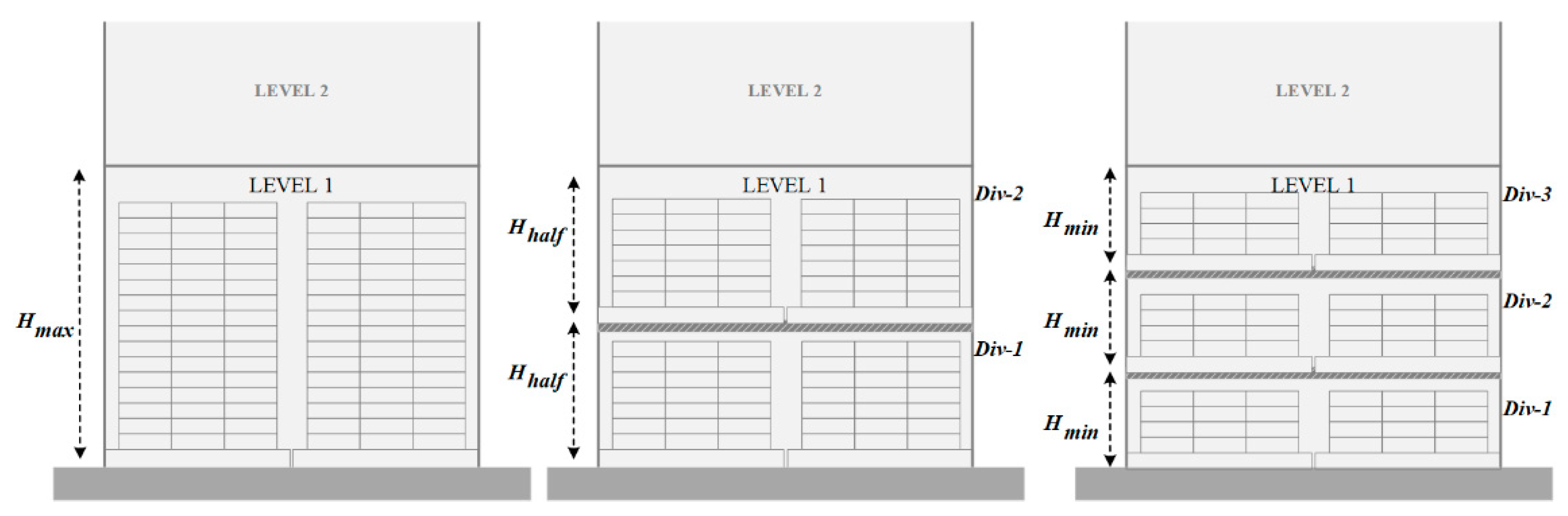
The present work is divided into two stages. The first stage addresses a storage location assignment problem focused on divisible horizontal locations, generating more storage positions of lower height (see Figure 1). This problem will be called Storage Location Assignment Problem with Variable Height or SLAP-VH.

In this way, SLAP-VH considers selecting locations to store products based on their demands, positioning customer’s most requested items near the exit, maintaining the priority of stackability (a factor that determines ergonomic efficiency), and arrange them in a way that minimizes cranes travel during operations.

In this work, SLAP-VH has been approached through mathematical programming and solved from its decomposition into four subproblems, which are solved sequentially. The subproblems correspond to assignment models based on an estimate of the collection route, i.e., the result determines the best position for each SKU considering the minimum travel distance in a linear way for the accommodation route, starting from the main route with side trips within aisles, and considering serpentine selection performed by an operator to assemble an order.

The second stage of the work consists of the economic evaluation of the crane path, based on the solution found by the proposed model, for two different analysis scenarios: one based on a random class-based storage strategy, and the other scenario is based on a storage strategy purely by class, where two decision criteria are defined to select the best storage route.

The rest of this article is organized as follows: a literature review is presented in Section 2; Section 3 describes the study warehouse and the approach to the problem that motivated the proposed methodology; Section 4 presents the global model of SLAP-VH; Section 5 presents the decomposition of the SLAP-VH problem and the models for each subproblem; Section 6 defines the proposed solution methodology; the assessment of the scenarios is described in Section 7; Section 8 and Section 9 presents the results obtained and the comparison of scenarios; Section 10 presents the discussion of the results; Section 11 provides final comments and conclusions.

2. Previous Literature

Slotting optimization research can be divided into two areas. The first is the modeling of the slotting process to improve efficiency in order preparation, load movement, handling of heavy over lightweight items, among others. And the second area is related to model resolution, using for example, exact, heuristic, and/or metaheuristic algorithms, among others [9]. Several researchers have developed both mathematical and heuristic models to address Slotting related to the Storage Location Assignment Problem (SLAP). Some of these studies can be consulted in

Table 1. Main characteristics of the presented storage location assignment models.

Reference	Characteristic of the Model	Storage Strategy	Function to Optimize	Solution Method
[16]	Warehouse with Crossover- Aisles with one direction of movement.	Weight order.	Minimize total distance traveled.	Mathematical model programming language C. Simulation Microsoft Visual Basic 6.0.
[13]	Linear movement of objects.	Single storage.	Minimize the number of obstructive objects.	Mathematical programming model.Genetic algorithm (GA).
[15]	Based on the principle of lower energy and shorter time.	Random.	Minimize total energy consumption. Minimize storage time.	Discrete particle swarm optimization (PSO).
[11]	Storage of containers in a maritime terminal.	Category of containers.	Minimize travel distance and time required load transfer.	Mixed-integer programming model. Hybrid stacking algorithm sequence procedure.
[18]	Travel distance considering three axes.	Symmetric storage.	Minimize total travel distance.	Mathematical model evaluated in LINGO Software.
[19]	Stored cycle travel times and double-depth retrieval.	Random. Always positioned first to the second lane.	Minimize travel time.	Analytical model. Simulation.
[20]	Warehouse symmetrical storage locations for a single product. Considers two horizontal axes and one vertical.	Symmetric storage.	Minimize total travel distance.	Mixed-integer programming model. Metaheuristics: Differential evolution (DE), Global optimization of the local and near neighbor particle swarm (GLNPSO).
[21]	Placing of accommodation lots with a fleet of k homogeneous teams.	Priority rule FCFS (First Come First Served).	Minimize the total time of lot formation.	Statistical design of divided parcels. Metaheuristic of intelligent neighborhood search (INS).
[1]	Bi-objective. Storage of blocks of pallets with storage locations for a single product.	Random.	Minimization of the total travel distance. Maximization of the average use of storage.	Mathematical model and a constructive heuristic algorithm.
[12]	Storage and recovery. Storage location for a single product.	Random.	Minimize travel time. Secondary function: maximize storage use.	Decomposition of 3 subproblems. Metaheuristic methods: Random, priority rule, and Genetic Algorithm.
[14]	Storage of homogeneous characteristics and WMS integration.	FIFO rule (First In First Out).	Minimize total costs.	Optimization model. Taboo search metaheuristic. Empirical rule.
[22]	Application of new storage strategy.	The selection area is divided into two sections called free seats and start locations.	Minimize the time required for order preparation.	Simulation (FlexSim). Matlab.
[23]	The model is based on correlated data products parameters, clients’ orders and warehouse layout.	Correlated data from the analysis of the ABC, XYZ, EIQ, AHP and COI indices.	Ensure the shortest time to access products of the highest frequency from the gates	software Pickup Simulo codified in PHP language and MySQL relational databases. Application of artificial neural networks
[24]	Machine Learning techniques for Product Allocation Problem	Product classification strategy comparing with reference picking data	Minimization of statistical dispersion indicators and maximization of clustering quality using Calinski-Harabasz criterion	Simulation using feed-forward artificial neural network and automatic clustering

, where the models developed tend to be very complex due to the SLAP NP-Hard complexity. In this sense, ref. [10] affirm that most of the storage and recovery problems fall into this category, which motivates the use of heuristics for their resolution. Besides, certain investigations propose decompositions of the problem, where initially the number of locations is addressed and the assignment is considered afterward. Using this strategy, ref. [11] addressed the SLAP for outbound containers in a maritime terminal, which was divided into two stages. They first determined the number of locations from a mixed-integer linear programming model and then defined the exact storage location based on a hybrid sequence stacking algorithm. This experimental study demonstrated effectiveness in comparing and analyzing performance in total travel distance between the yard and the bunk, the imbalance of the workload between different blocks of containers, and the percentage of repetitions in loading operations. In this way, the hybrid sequence stacking algorithm reduces the unnecessary movement of containers in cargo operations to 18%, compared to 30% of the average rehandle percentage in the case study analyzed.

It is interesting to note that the vast majority of the studies carried out consider as an objective function the minimization of time, cost, or distance. However, authors such as [12] developed a mathematical model that minimizes storage time by incorporating a two-objective optimization approach: maximization of space availability and minimization of production due date measurements. Ref. [1] developed a mathematical model that considers two simultaneous goals: minimize travel distance and maximize average storage usage. The SLAP-VH also incorporates this feature, considering the minimization of cranes route as the main objective function, and the maximization of storage use as a secondary function.

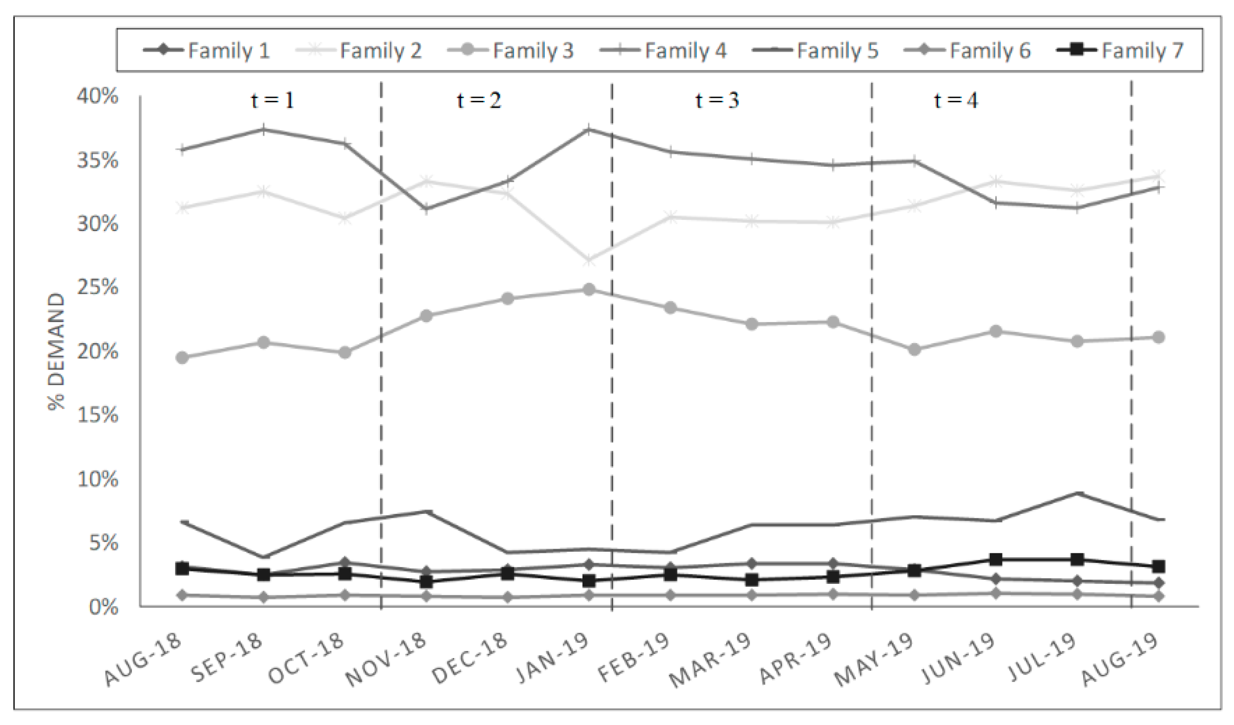
One of the main parameters of the SLAP modeling is the planning horizon. Research in the field reveals that evaluation periods adjusted to the problem achieve greater effectiveness in the correct arrangement of SKUs. For example, in [13] was defined the time horizon in periods of discrete units (days) to consider the real situation of the research, where the storage warehouse releases outgoing objects and stores incoming objects in each unit period. For the case of SLAP-VH, the period ($t$) is based on the normal distribution of the demand for each SKU (see Figure 2), this allows the Slotting to be defined as active since the correct accommodation adapts to the temporality of the products according to the defined periods.

The models proposed by the researchers are commonly solved by heuristics or metaheuristics, considering the complexity of the SLAP. However, these heuristic and metaheuristic algorithms are not able to guarantee the optimality of the solutions, although, in some cases, they offer nearly optimal solutions depending on the execution times and the parameter setting. Researchers have evaluated the effectiveness of different algorithms for the SLAP. For example, ref. [14] made a comparison between an optimization method, a Tabu Search metaheuristic, and an empirical rule. The authors concluded that the size of the accommodate list has a significant effect on its structure and the optimality of the results. Additionally, the optimization method reduced labor costs compared to the solutions provided by metaheuristics. Reducing costs has a strong impact on the entire order picking process since all activities are connected. Ref. [15] state that the optimization of positioning not only reduces costs and energy in the operation but also improves the efficiency of the storage of goods. Therefore, optimizing the Slotting process helps to complete orders at a faster pace, benefiting the consolidation work (i.e., a process that groups the demand for orders from different areas, into complete orders), and the service level delivered to end consumers. Managers want to reduce the time spent on movements within the warehouse, not only to decrease labor cost and production downtime but also to shorten customer response time. Ref. [16] developed a study of the time of the activities carried out in the preparation of orders in Maines Paper and Food Services (Inc in Conklin, NY), concluding that 40% of the time is spent on travel. Therefore, reducing this percentage could significantly save a warehouse operating expense. Reducing travel time implies reducing the distance of cargo transfer and therefore the number of operators required to place an order. Ref. [17] state that the distance largely depends on the design of the warehouse. It is logical, in the case of slotted storage, to place the merchandise that has a high turnover in privileged locations close to the dispatch point. In contrast, when placing an order where items need to be selected in a single tour, it makes more sense to assign SKUs to locations that minimize travel time for routes.

On the other hand, travel time depends entirely on the location of the SKUs in the warehouse and, in turn, on the storage strategy. The latter is an important factor in warehouse performance, since optimizing the slotting process consists of optimizing storage locations based on the characteristics of the racks and also the requirements of the processes within the warehouse.

Given the above, this work proposes an optimization model for the Slotting process (SLAP-VH), where its distinctive feature is the consideration of a warehouse whose locations corresponding to the first accommodation level are divisible. To the best of our knowledge, this feature has not been previously considered within SLAP literature. This work is divided into two stages: determining the optimal location for each SKU in a planning horizon with four defined periods, and determine the best of two allocation scenarios to reduce travel distance and costs. SLAP-VH is solved through a mixed-integer linear programming model (MILP), considering a representative sale day belonging to the most critical period (highest number of orders). The choice of the solution method addressed for SLAP-VH was determined from a comparative table between three metaheuristics and an optimization method (namely: PSO, GA, Tabu Search, and optimization), where the high execution times of the metaheuristics motivated the construction of these evaluation scenarios, solving them from a MILP optimization model with the Gurobi solver through an exact procedure. On the other hand, the combination of storage locations (racks and floor locations) is a unique feature compared to the optimization models investigated, in addition to the incorporation of four outputs from the warehouse under study. The main characteristics of the study problem compared to the research carried out are presented in

Table 2. Attributes of SLAP-VH.

Model Characteristics	Storage Strategy	Function to Optimize	Solution Method
Warehouse with four outputs. Storage in Racks and storage a floor. Locations in first accommodation level with multi-level.	Two storage scenarios: Storing by random classes Storage purely by classes	Minimize travel cranes. Maximize storage use.	Mathematical programming model MILP. Python programming language, Pyomo Gurobi solver.

.

The literature reviewed in this research shows how the storage location assignment problem has been addressed in different warehouses. None of the models proposed by the reviewed authors solves the problem with different types of storage locations and divisible locations developed in this paper; however, they provide relevant factors to consider in storage strategies and problem modeling for locations storage both in-floor locations (“Perchas”), described by [1], and also in racks, developed by [12]. Besides, this latter considers the subdivision of the assignment problem, influencing the development of this research. On the other hand, the objective proposed in this work is equivalent to most of the models addressed in the state-of-the-art literature, that is, to reduce the travel time of cranes or to minimize the operating cost of the warehouse picking operation, functions that are strongly related. Therefore, combining and adapting the models presented in the literature to the proposed problem allows to obtain nearly optimal solutions, minimizing time, cost, and also increasing the warehouse space utilization.

3. Warehouse Description and Methodology

The mathematical model is built and evaluated based on real data from a distribution center (DC) of a beverage company that supplies Chile and neighboring countries, provided with around 1200 SKUs on inventory in its dependencies. The DC picking area is modeled to develop the SLAP-VH, where the SKUs are represented as loaded pallets of homogeneous dimensions. As can be seen in Figure 3, the warehouse is composed of columns of racks with equal height and the same number of slots. The width and depth of the storage positions of racks are the same for the entire warehouse with dimensions $1\times 1.2$ m². The height varies between $0.7$ m to $1.2$ m according to the division of the location and SKU format dimensions. Thus, there are three operations ($o$) where only one of them can be applied for each location, that is: the location cannot be divided, can be divided into two parts, or can be divided into three parts.

Warehouse aisles correspond to the space between each rack, which are listed from left to right. The design of the warehouse is represented as a rectangular section, where the entrance of the cranes to the locations are on both sides of the aisle, except for the first and last side. Additionally, the warehouse has four exits to the consolidation and dispatch area.

Into the warehouse, only trilateral cranes are considered with one operator onboard and an average speed of 5 km/h, where minimizing the distance of crane movements allows determining the number of trips during an 8-h shift, concluding in this way the number of operators needed to satisfy the requirements. This fact, however, can be addressed with greater depth in future researches.

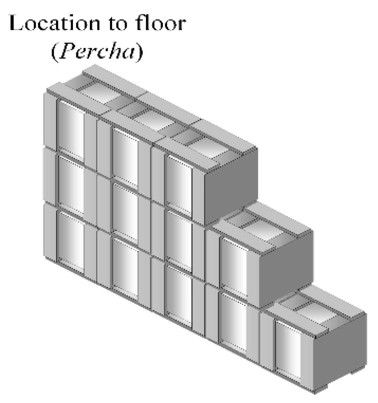
In the warehouse under study, there are three storage considerations: (a) locations should be assigned to the pallets according to affinity; (b) The pallets with the highest demand should ideally be assigned in locations without division, and; (c) two columns of locations, which do not include racks, cannot be divided. These columns are called “Perchas”. These are worked separately, treating as a fourth subproblem for SLAP-VH.

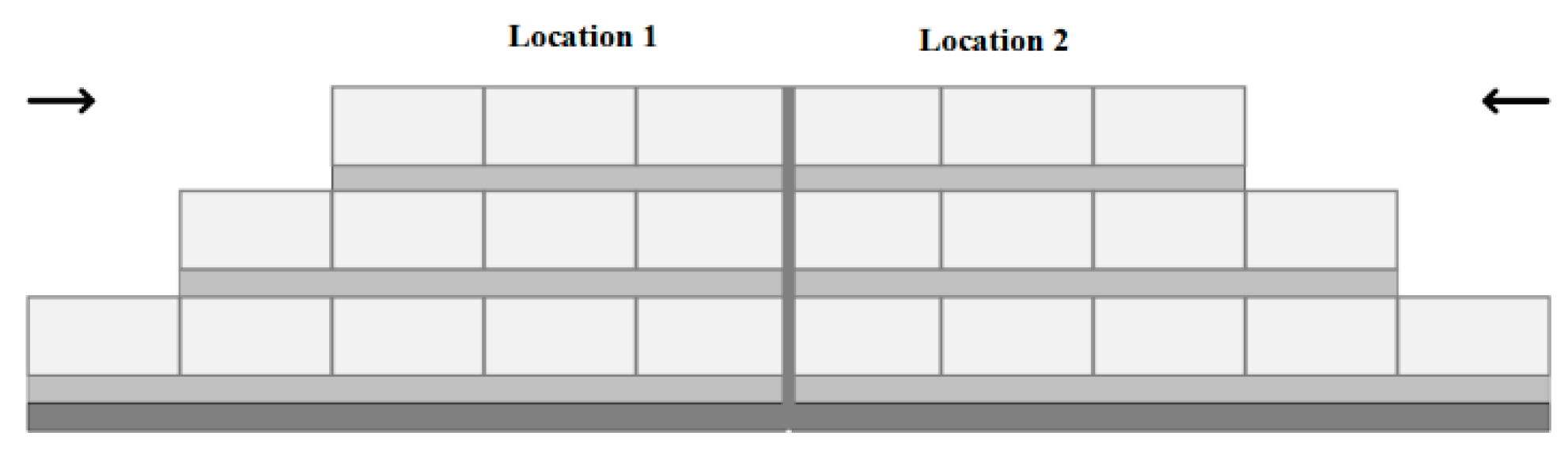
Perchas are locations stacking pallets that are stored on the floor at the top, arranged in stacks. This area is managed according to the dedicated storage strategy, since, as shown in Figure 4, each location has capacity for twelve pallets, that is, five pallets can be assigned in base and depth, and then start to be stacked while maintaining ergonomics and operator protection. It is important to store only one type of SKU for each Percha location, since a great storage depth generates inconveniences such as, for example, not finding a pallet of SKU “A” since it is under a stack of SKU pallets “B”. In other cases, this situation can cause the operator may forget that they stored a pallet under other SKUs, passing the expiration date. Regarding time, stacking pallets of different SKU types demands the operator to spend more time searching and moving the necessary pallets until reaching the desired one.

The decision to divide locations is based on the demand for the products: for example, if an SKU is less requested in a period, this will be assigned to locations of smaller capacity and further from the warehouse. The opposite happens with a highly demanded SKU, which will be assigned to a high capacity location and close to the exit. Finally, the Perchas are locations defined by the company for a certain type of SKU where the decision consists of positioning the pallet according to its proximity to the exit point since these locations are not divisible.

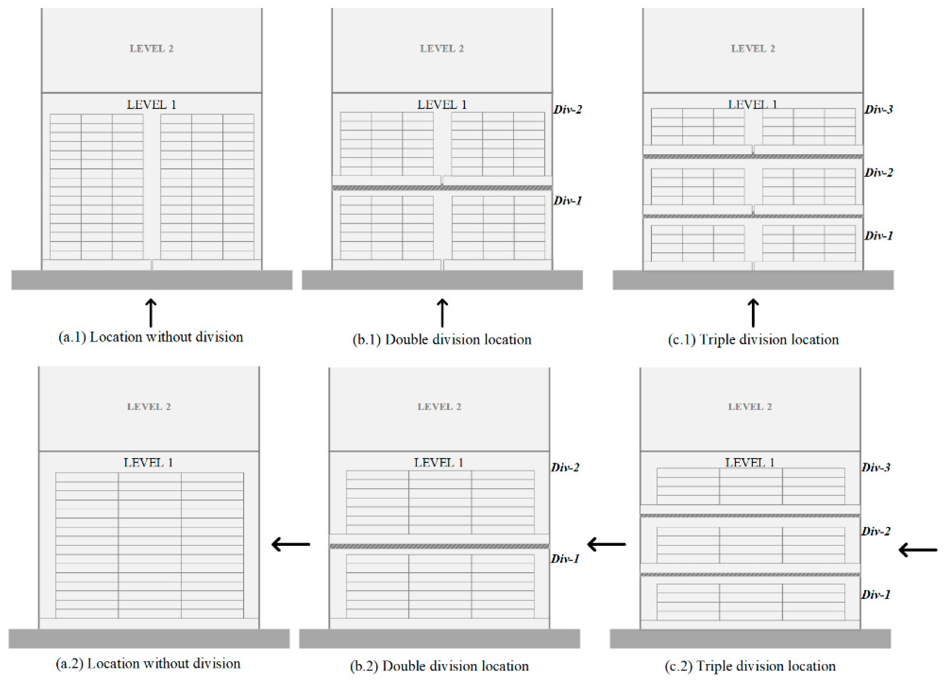
SLAP-VH only considers the first-level stacking locations, that is, the first location from the floor of each rack. Storage is governed by order priority rules, specifically by EDD (Earliest Due Date), except for the picking slots, corresponding to the first level of accommodation. For this reason, this research focuses exclusively on the assignment of these locations, which can be divided into three positions, in two, or they can be maintained without performing any division. In this sense, three, two, or one pallet can be stored respectively. Each first-level storage slot has capacity for two pallets of maximum height (Figure 5(a.1,a.2)), while a divided slot (Figure 5(b.1,b.2)) has capacity for four medium height pallets, or six pallets of minimum height (Figure 5(c.1,c.2)). Therefore, the term “location” will be used to denote the storage space of a rack with a capacity of one pallet of maximum height, while the storage space of a divided slot of less height will be called “position”.

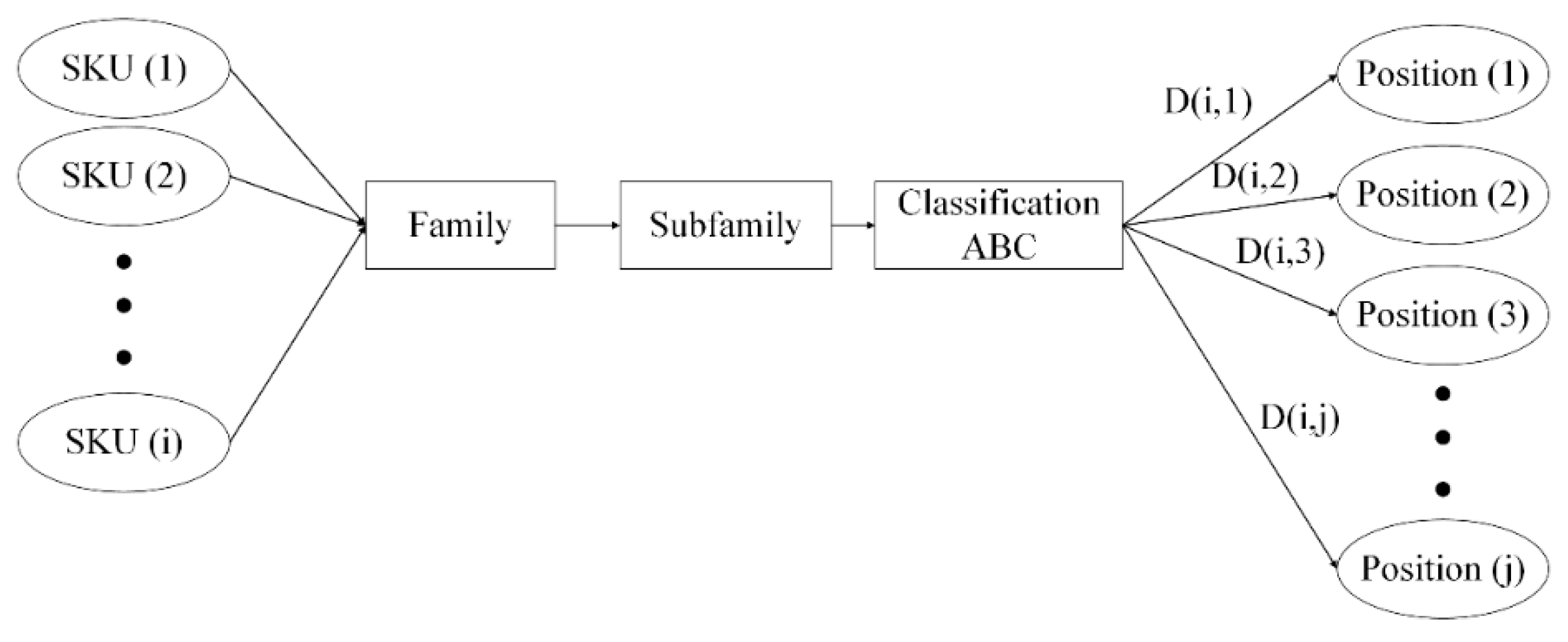
Within the warehouse, SKUs are classified based on the Pareto principle according to the class or product family to which they belong, where $80\%$ of the total quantity demanded corresponds to type “A” SKUs, $15\%$ to the “B” and $5\%$ to the “C”. The ABC classification is essential to know the need for accommodation of each SKU based on its demand. Each of the families has a different number of SKUs and each family has a regrouping called a subfamily, which is based on the weight of the products. In this way, the grouping by families only allows determining the product category, while the regrouping by subfamilies allows classifying with more information about each SKU based on the size of the product. This creates a greater connection between stackability priority and affinity between the products. In this sense, it is necessary to clarify that grouping by product families and sub-families is a strategy defined by the company, which is enhanced by the ABC classification by periods. Initially, there were 12 families, however, in order to group those with a smaller quantity without affecting stackability, 7 families were finally obtained.

As [3] indicates, the general assignment problem is classified as an NP-hard complexity problem. From this statement, SLAP-VH can also be considered as an NP-hard problem, since it applies a stricter constraint set for the general storage assignment problem. The case study considered $726$ SKUs that must be distributed in $1170$ locations, a value that may increase considering the division of locations. Therefore, evaluating all the possible combinations becomes an impractical strategy given the order compilation time $O\left(n!\right)$ for exact algorithms. However, based on the assumptions used and presented in

Table 3. Main assumptions considered in SLAP-VH.

The Warehouse Starts Empty to Accommodate SKUs Packing

All accommodation operations are performed by homogeneous cranes

Stored pallets are homogeneous and loaded by a single SKU

All SKUs must be stored in at least one location or position

All locations used in the problem corresponds to the first accommodation level

All locations can be divided, except for Perchas

The distance is measured with respect to the warehouse exits and the end of the aisle in a linear way

The distance is equal for both divided and without division locations

A not divided location is assigned when an SKU demands at least one pallet bin

A two-position location is assigned when an SKU demands between 0.5 and 1 pallet bin

A three-position location is assigned when an SKU demands less than half of a pallet bin

, the underlying complexity tends to decrease, reducing the number of decisions and the combination of cases that arise when trying to model reality. In this way, the presented model results in a mixed-integer linear programming problem (MILP).

It is important to consider that for modeling purposes, only the use of full storage pallets will be considered. This assumption applies since the cranes are loaded with either a full pallet or with a load conformed for different clients until creating a complete pallet, given the volume of demand of the company. It should be noted that the full pallet denomination refers to a pallet loaded in its full storage capacity. In this sense, the operators move full pallets to a location or position and then return without cargo to repeat the packing operation, before the order picking process. In order picking, there are three different activities to move SKU pallets:

• Transfer of a complete pallet: the operator only transfers a pallet loaded with a single SKU to the nearest exit. This activity is normally done when an SKU is highly demanded.
• Transfer of a replenishment pallet: the operator moves a complete pallet to a location or position when it has become empty during the picking operation.
• Transfer of a conformed pallet: the operator makes collection trips until a complete pallet is formed and goes to the closest exit.

These activities are considered in the evaluation of scenarios through the picking operation once the product layout has been obtained.

Appendix A lists the notations, abbreviations, and symbols used in the document.

4. Global Solution Model

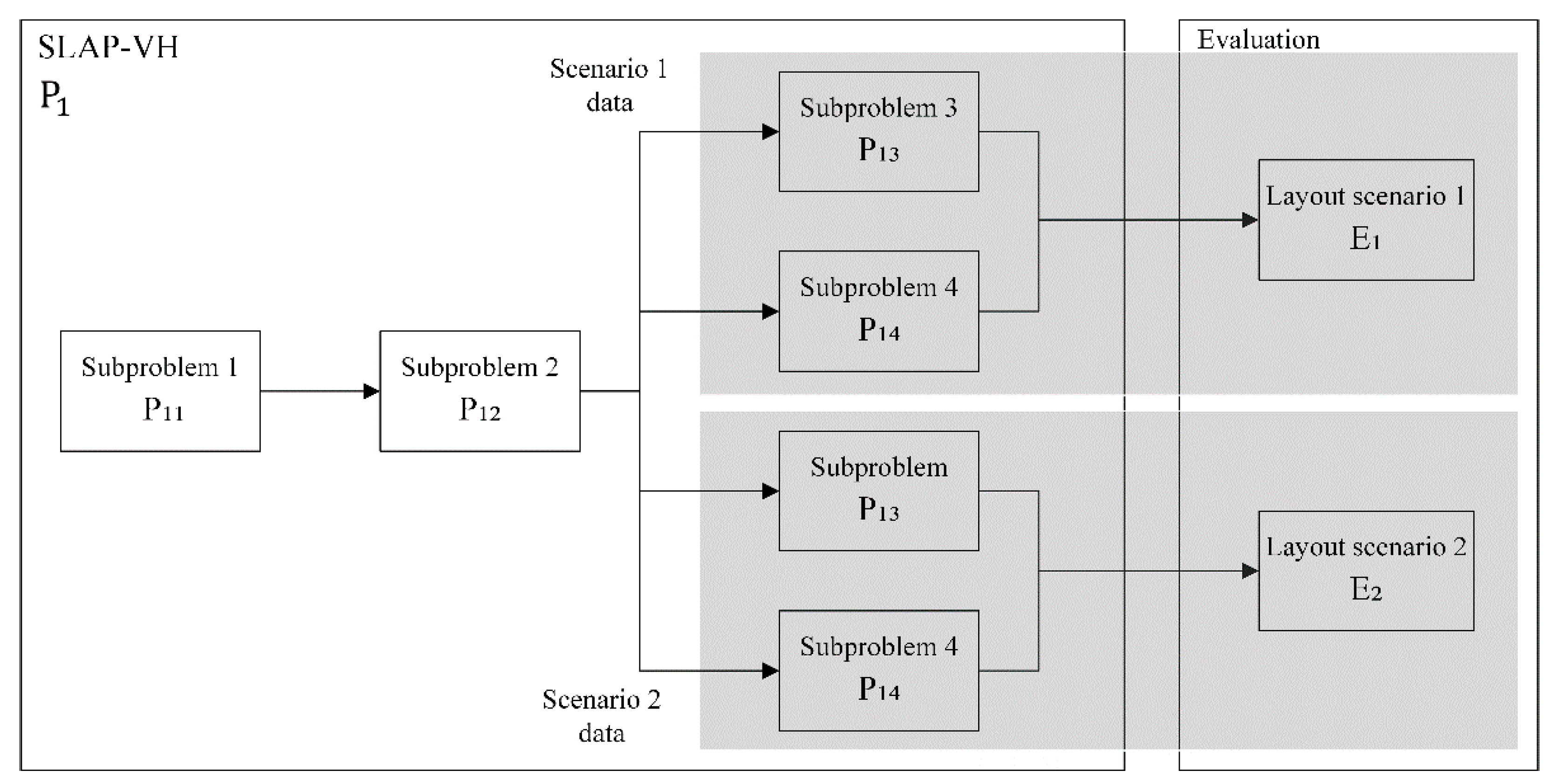
In this section, the global model of SLAP-VH is presented, which will be denominated $P_1$, as can be seen in Figure 6. The problem begins by solving the first subproblem, which determines the number of locations through the demand for the SKUs, to continue with the second subproblem, and start the construction of the two different Slotting scenarios. Once the results obtained are known, we proceed to the third subproblem, defining which locations should be divided. In parallel, the fourth subproblem is solved to later introduce the results obtained in the global model of $P_1$. The specifications of each subproblem are defined in the next section. It is necessary to clarify that the sequentiality in the development of the problem is determined from the key decisions considered in Section 5, since the simultaneous resolution of the analyzed subproblems does not allow obtaining feasible scenarios. Finally, the SLAP-VH solution is reflected in two slotting layout scenarios, which are evaluated to determine the optimal solution in terms of distance and costs. These scenarios show the three types of storage strategies that have been applied in the warehouse under study. Since locations without racks already have a defined strategy, the two scenarios defined in Section 7 are generated.

The mathematical model proposed for $P_1$ aims to determine which is the best position for each SKU within the warehouse that minimizes the travel distance of cranes, considering the ABC classification and the stackability priority. The relevant parameters and decision variables are presented in Appendix A.

The formulation of the model $P_1$ is presented below:

$$Min {\displaystyle \sum }_I{\displaystyle \sum }_J{\displaystyle \sum }_K\left(Y_{ji}·D_{jk}·value\_sk{u}_i\right)$$

(1)

Subject to

$${\displaystyle \sum }_S{\displaystyle \sum }_I\left(Y_{ji}·sku\_subfamili{y}_{si}·position\_subfamil{y}_{js}\right)=1,\hspace{1em}\forall j \in J$$

(2)

$${\displaystyle \sum }_J(Y_{ji}·typ{e}_{jo})\ge sku\_typ{e}_{io},\hspace{1em}\hspace{1em}\forall i \in I, o \in O$$

(3)

The objective of the proposed problem is to secure to each SKU at least one location, considering the minimum distance from the warehouse exit. Constraint set (2) establishes that each location/position must have a single SKU, and in set (3) it is determined that an SKU can have more than one location/position. Both restrictions consider the type of operation that position has, and the family to which it corresponds.

5. Decomposition of the Problem

The problem $P_1$ with its corresponding objective function $F_1$ is divided into four subproblems, called $P_{1.1}$, $P_{1.2}$, $P_{1.3},$ and $P_{1.4}$, where their corresponding objective functions are called $F_{1.1}$, $F_{1.2}$, $F_{1.3},$ and $F_{1.4}$ respectively. These are solved sequentially, where the result of each one is used as input to the immediately following subproblem. Each subproblem determines the following key decisions: (1) Number of locations to divide, (2) assign product family per aisle, (3) sort according to stackability priority within the aisle and define the location to be divided, and (4) define the number of locations for each family that go to Perchas sorting by subfamily. As stated above, it is common to solve these subproblems separately considering their complexity, although they are strongly interconnected [25].

Table 4. List of addressed problems, and objective functions considered in each problem.

Abbreviation	Description
SLAP-VH or $P_1$	Storage location assignment problem with variable height
$P_{1.1}$	Subproblem of $P_1$ that determines how many locations to divide
$P_{1.2}$	Subproblem of $P_1$ that assigns families to aisles
$P_{1.3}$	Subproblem of $P_1$ that determines which locations to divide
$P_{1.4}$	Subproblem of $P_1$ that determines how many locations correspond to each family that goes to Perchas
Abbreviation	Description	Related Problem
$F_1$	Minimize the distance from an SKU to the warehouse exit	$P_1$
$F_{1.1}$	Minimum number of divided locations	$P_{1.1},P_{1.2}$
$F_{1.2}$	Affinity analysis	$P_{1.2},P_{1.3}$
$F_{1.3}$	Minimize the distance, from a location to warehouse exit	$P_{1.3},P_1$
$F_{1.4}$	Minimize the number of locations for “B” classification SKUs	$P_{1.4},P_1$

presents a list of the problems studied in this research.

In $P_1$, locations are assigned to each SKU from the results obtained from $F_{1.1}, F_{1.2}, F_{1.3},$ and $F_{1.4}$, where each subproblem considers different search spaces to determine key decisions. Appendix A shows the main parameters and decision variables used in the models for each subproblem.

5.1. Subproblem $P_{1.1}$: Locations to Divide

The model for $P_{1.1}$ is presented below, in which the decision variables define the quantity of simple, double, and triple locations that each SKU must occupy.

$$Min {\displaystyle \sum }_I\left(\frac{uB{2}_i}{2}+\frac{uB{3}_i}{3}+\frac{uC{2}_i}{2}+\frac{uC{3}_i}{3}\right)$$

(4)

Subject to:

$$total\_UA\ge {\displaystyle \sum }_{I}u{A}_i$$

(5)

$$total\_UB\ge {\displaystyle \sum }_{I}u{B}_i$$

(6)

$$total\_UB2\ge {\displaystyle \sum }_I\frac{uB{2}_i}{2}$$

(7)

$$total\_UB3\ge {\displaystyle \sum }_I\frac{uB{3}_i}{3}$$

(8)

$$total\_UC\ge {\displaystyle \sum }_{I}u{C}_i$$

(9)

$$total\_UC2\ge {\displaystyle \sum }_I\frac{uC{2}_i}{2}$$

(10)

$$total\_UC3\ge {\displaystyle \sum }_I\frac{uC{3}_i}{3}$$

(11)

$$\begin{array}{c}total\_locations\ge total\_UA+total\_UB +total\_UB2 +total\_UB3 +total\_UC\hfill \\ \hspace{1em}\hspace{1em}\hspace{1em}\hspace{1em}\hspace{1em}\hspace{1em}\hspace{1em}+totaL\_UC2+total\_UC3\hfill \end{array}$$

(12)

$$\begin{array}{c}u{A}_i\ge \alpha \ast dda\_location{s}_i\\ \hspace{1em}\hspace{1em}\hspace{1em}\forall i \in I \end{array}$$

(13)

$$\begin{array}{c}\hspace{1em}\hspace{1em}\hspace{1em}\hspace{1em}\hspace{1em}\hspace{1em}u{A}_i=1\hfill \\ \forall i \in I: dda\_location{s}_i=0\wedge SKU\_A_i=1\hfill \end{array}$$

(14)

$$\begin{array}{c}u{B}_i\ge \beta \ast dda\_location{s}_i\\ \hspace{1em}\hspace{1em}\hspace{1em}\hspace{1em} \forall i \in I: SKU\_B_i=1\end{array}$$

(15)

$$\begin{array}{c}\hspace{1em}\hspace{1em} u2B_i\ge dda\_decima{l}_i\hfill \\ \forall i \in I: dda\_decima{l}_i\ge \gamma \wedge SKU\_B_i=1\hfill \end{array}$$

(16)

$$\begin{array}{c}\hspace{1em}\hspace{1em} u3B_i\ge dda\_decima{l}_i\hfill \\ \forall i \in I: dda\_decima{l}_i\le \gamma \wedge SKU\_B_i=1\hfill \end{array}$$

(17)

$$\begin{array}{c}u{C}_i\ge \beta \ast dda\_location{s}_i\\ \hspace{1em}\hspace{1em}\hspace{1em}\hspace{1em} \forall i \in I: SKU\_C_i=1\end{array}$$

(18)

$$\begin{array}{c}\hspace{1em}\hspace{1em} u2C_i\ge dda\_decima{l}_i\hfill \\ \forall i \in I: dda\_decima{l}_i\ge \gamma \wedge SKU\_C_i=1\hfill \end{array}$$

(19)

$$\begin{array}{c}\hspace{1em}\hspace{1em} u3C_i\ge dda\_decima{l}_i\hfill \\ \forall i \in I:: dda\_decima{l}_i\le \gamma \wedge SKU\_C_i=1\hfill \end{array}$$

(20)

$$total\_locations\le loc\_total$$

(21)

$$\begin{array}{c}total\_sum{2}_s\ge \frac{{\sum }_I\left(uB{2}_i+uC{2}_i\right)·sku\_subfamil{y}_{si}}{4}\\ \hspace{1em}\hspace{1em}\hspace{1em}\hspace{1em}\hspace{1em} \forall s \in S \end{array}$$

(22)

$$\begin{array}{c}{\displaystyle {\displaystyle \sum }_I}\left(uB{2}_i+uC{2}_i\right)·sku\_subfamil{y}_{si}-total\_sum{2}_s·4=0\\ \hspace{1em}\hspace{1em}\hspace{1em}\hspace{1em} \forall s \in S\end{array}$$

(23)

$$\begin{array}{c}total\_sum{3}_s\ge \frac{{\sum }_I\left(uB{3}_i+uC{3}_i\right)·sku\_subfamili{y}_{si}}{6}\\ \hspace{1em}\hspace{1em}\hspace{1em}\hspace{1em}\hspace{1em} \forall s \in S \end{array}$$

(24)

$$\begin{array}{c}{\displaystyle {\displaystyle \sum }_I}\left(uB{3}_i+uC{3}_i\right)·sku\_subfamili{y}_{si}-total\_sum{3}_s\ast 6=0\\ \hspace{1em}\hspace{1em}\hspace{1em}\hspace{1em} \forall s \in S\end{array}$$

(25)

The objective is to minimize the number of total double and triple divisions in the warehouse. Constraints sets (5) to (11) indicate the total number of simple, double, and triple locations. In (12), the total amount of locations obtained is grouped, which are limited by equation (21). Constraints sets (13) to (20) guarantee the coverage of locations according to the ABC classification of the SKUs, reflected in the parameters $\alpha , \beta , \gamma$. Expressions (22) and (23) consider that the number of double locations for each subfamily is divisible by 4. The previous condition is also considered in (24) and (25), where the number of triple locations for each subfamily is divisible by 6.

5.2. Subproblem $P_{1.2}$: Allocation of Families to Aisles

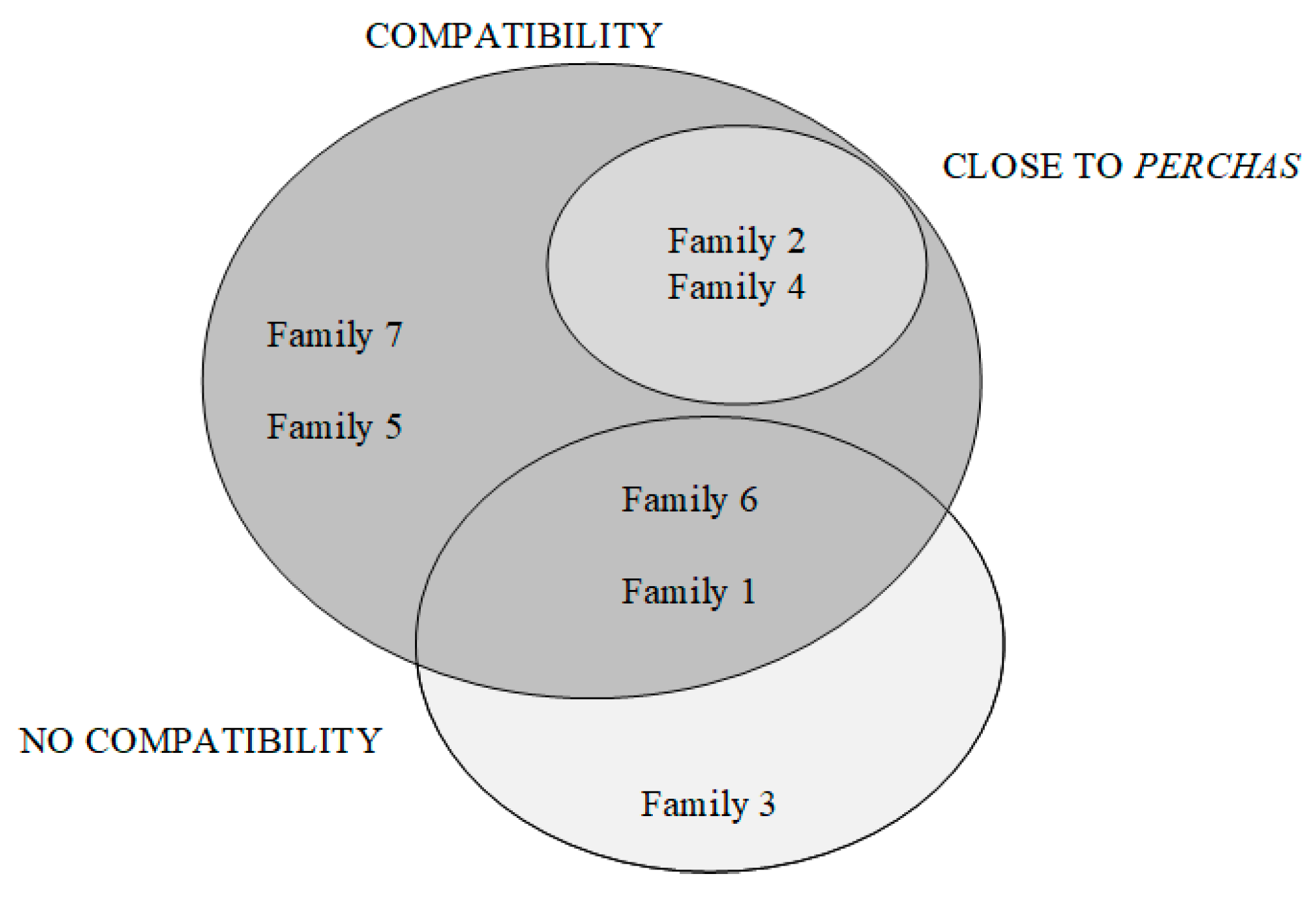
This subproblem has been approached from the experience with the affinity between the studied families, which aims to define those families that should be assigned close to one another. It is possible to highlight three main classifications to determine affinity: (1) SKUs that belong to different families and are commonly requested together by the customers; (2) SKUs that are not frequently requested, and therefore have no affinity with other SKUs of other families, and; (3) given that Perchas have greater storage capacity per location, those SKUs that are less demanded by customers and belong to the families in Perchas are considered to be positioned near these locations.

Table 5. Affinity or compatibility between families.

Compatibility		Closeness to Perchas	Without Compatibility
Family 1	Family 6	Family 2	Family 3
Family 2	Family 4	Family 4	Family 1
Family 7	Family 5		Family 6

describes the analysis carried out from the families under study.

The affinity between families allows determining the physical storage arrangement within the aisles. Assigning families to aisles, that is, constructing accommodation lines, facilitates the work of operators when traveling along the aisle selecting only what is necessary, without going back or travel long distances when making the collection route.

5.3. Subproblem $P_{1.3}$: Determine Which Location to Divide

To determine which locations should be divided, the following linear programming problem is proposed:

$$Min {\displaystyle \sum }_S{\displaystyle \sum }_J{\displaystyle \sum }_{K}X{0}_{js}{D}_{jk}\left(\frac{1}{weigh{t}_s}\right)$$

(26)

Subject to

$$\begin{array}{c}{\displaystyle {\displaystyle \sum }_J}X{0}_{js}\le ub{0}_s\\ \hspace{1em}\hspace{1em}\hspace{1em}\forall s\in S\end{array}$$

(27)

$$\begin{array}{c}{\displaystyle {\displaystyle \sum }_J}X{2}_{js}\le ub{2}_s\\ \hspace{1em}\hspace{1em}\hspace{1em}\forall s\in S\end{array}$$

(28)

$$\begin{array}{c}{\displaystyle {\displaystyle \sum }_J}X{3}_{js}\le ub{3}_s\\ \hspace{1em}\hspace{1em}\hspace{1em}\forall s\in S\end{array}$$

(29)

$$\begin{array}{c}{\displaystyle {\displaystyle \sum }_S}\left(X{0}_{js}+X{2}_{js}+X{3}_{js}\right)=1\\ \hspace{1em}\hspace{1em}\hspace{1em}\forall j\in J\end{array}$$

(30)

The objective function of the subproblem $P_{1.3}$ is to minimize the distance from simple locations to the exit, for each family according to the priority order. Constraints sets (27), (28), and (29) determine the number of locations that will not be divided, or otherwise divided into two and three, respectively. Constraint set (30) establishes that each location can only perform one operation.

5.4. Subproblem $P_{1.4}$: Perchas

The mathematical model for $P_{1.4}$, has the objective to determine the necessary number of locations (see Figure 7) for each SKU of families that must be positioned on Perchas.

$$Min {\displaystyle \sum }_I{u}_{i}sku\_b_i$$

(31)

Subject to

$$total\_per\ge {\displaystyle \sum }_I{u}_i$$

(32)

$$\begin{array}{c}\hspace{1em}\hspace{1em}\hspace{1em}{u}_i\ge 1\hfill \\ \forall i \in I \mathrm{with} dda\_locations\le \theta \hfill \end{array}$$

(33)

$$\begin{array}{c}1\le u_i\le \mu \ast dda\_location{s}_i\hfill \\ \hspace{1em} \forall i \in I con dda\_locations>\theta \hfill \end{array}$$

(34)

The objective function in (31) corresponds to the minimization of the number of locations for those SKUs that are rated as “B”. Constraint (32) establishes that the total number of locations must not exceed the number of available locations. Constraints sets (33) and (34) determine the number of locations according to the ABC classification of the SKUs, reflected in the parameters $\theta \mathrm{and} \mu$.

5.5. General Algorithm

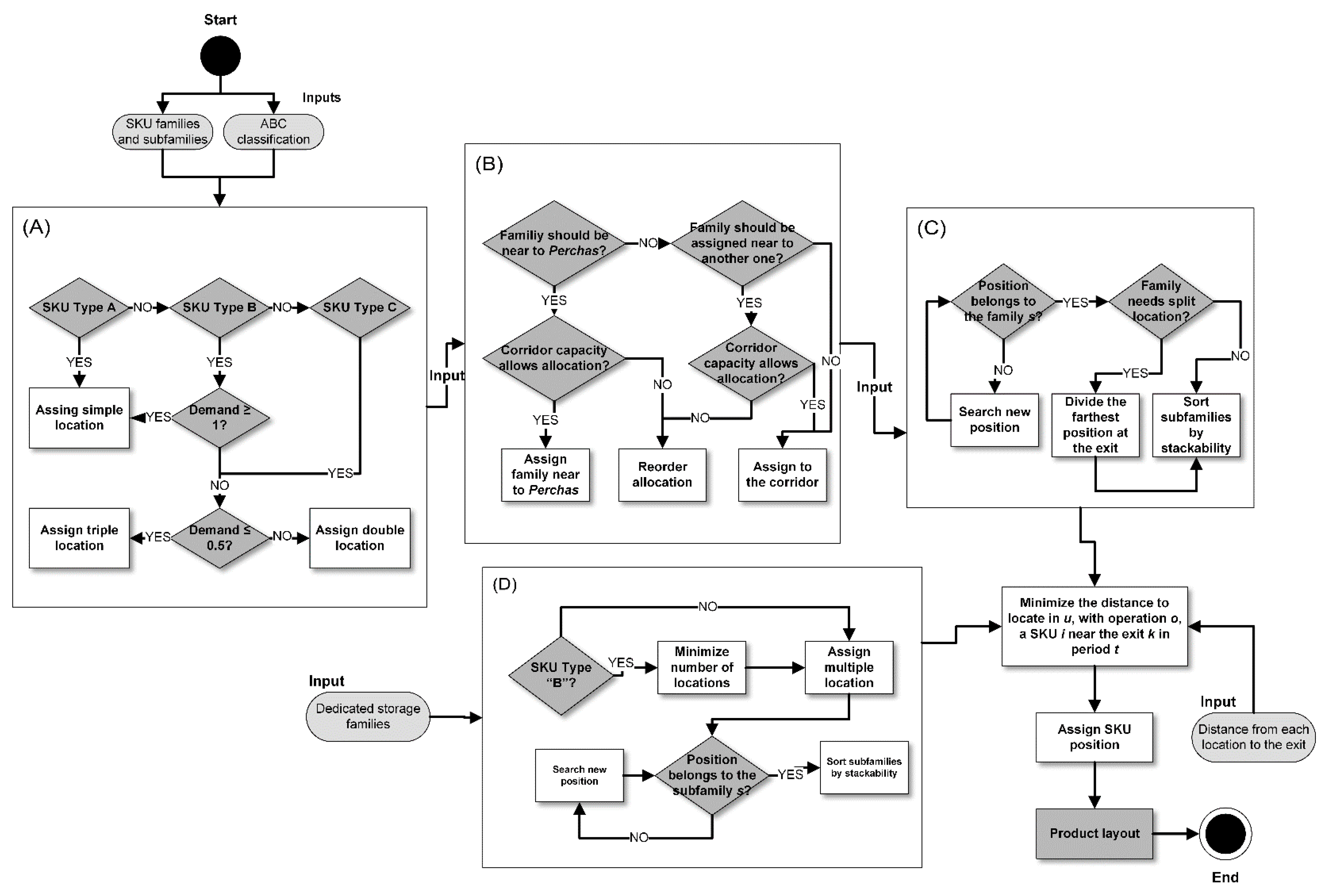
A flow diagram is built to solve the global model, which establishes the inputs required for each subproblem graphed in Figure 8, where (A), (B), (C), and (D) correspond to key decisions that solve the subproblems $P_{1.1}, P_{1.2}, P_{1.3 }$, and $P_{1.4}$ respectively, ending with the assignment of locations in $P_1$. The details of each step are described in the next section.

6. Proposed Methodology

This section defines the proposed solution models to address each subproblem.

6.1. Solution Approach Proposed for $P_{1.1}$

The problem $P_{1.1}$ can be considered a variant of the integer linear programming demand satisfaction problem. The mathematical model presented defines demand as the number of locations that each SKU needs, which is satisfied with simple, double, or triple locations. The total demand for locations corresponds to a non-integer value, therefore, to obtain the best combination of possible operations, the maximum coverage is determined for SKUs, where those articles that demand more or equal capacity than a location can offer, requires the assignment of simple positions. If demand is less than one location, double locations must be assigned if it is between one or half pallet, and triple if it is less than half of a pallet.

The structure of the rack in storage space symbolizes two locations, therefore, it is not possible to divide a simple location, since if one of these is divided, the paired location must do so. Therefore, the number of double locations assigned by subfamilies must consider a multiple of four, and a multiple of six for triple locations.

The problem model $P_{1.1}$ is implemented using Python programming language and the Pyomo library. This mixed-integer linear optimization model (MILP) is solved using Gurobi optimizer. The problem involves $\mathrm{4,574}$ variables, $\mathrm{4,573}$ of an integer nature, and one continuous variable, in addition to $\mathrm{3,454}$ constraints and one objective minimization function.

6.2. Solution Approach Proposed for $P_{1.2}$

Family affinity and stackability priority require full attention from managers and operators. On the one hand, the incoming and outgoing products must be considered to accommodate them correctly and, on the other hand, the ergonomics of the pallet must be studied securing stability in its dimensions and weight, avoiding unsafe actions for the operators. In this way, the distribution of families and subfamilies is carried out based on affinity and stackability, merging the analyzed classification to the study warehouse, and finally generating the assignment order of subfamilies.

From Figure 9, a logical order emerges that addresses the priorities of assigning families to aisles. It is important to emphasize that the warehouse is inflexible, therefore, there is only one possible arrangement to meet the priorities considering the solution obtained in $P_{1.1}$, this is represented in Figure 10. It should be considered that the assignment of families to aisles must maintain the continuity of the family, i.e., not to position an “X” family in the first aisle and continue its assignment in the last. This helps operators to find products in aisles in a faster way. In this sense, it can be observed that those families that must go near the “Perchas” location are the closest, without interrupting the continuity of the following families. The same observation applies to those who have compatibility. Finally, the one that does not have compatibility, being the most numerous, is positioned in the aisles furthest from “Perchas” avoiding losing continuity.

6.3. Solution Approach Proposed for $P_{1.3}$

Once the families are assigned to each aisle and the division for locations are known, the objective of $P_{1.3}$ is to define which locations will be divided according to the number of locations assigned to each family. The assignment operation is done for those families with a large volume of SKUs since those with less than 10% of the total SKUs can be assigned manually, and the optimal result is predictable with respect to the priorities.

The model of this subproblem is coded, like the subproblem $P_{1.1}$, in Python language from the Pyomo software packages. The model is implemented with the mixed-integer linear optimization solver Gurobi, considering $\mathrm{13,717}$ variables used, being $\mathrm{13,698}$ of them of binary nature, $\mathrm{13,716}$ integer (including binary), and one continuous variable. Besides, $798$ constraints and one objective minimization function were considered. These values decrease as the number of SKUs per family decreases.

Once each position by families is defined, we proceed to sort by ABC classification, since the model’s solution sends all double and triple locations at the end of the aisles. Despite being the optimal global solution, it affects the grouping of subfamilies. On the other hand, the stackability priority is defined by the model, which remains fixed. The ABC classification allows defining the prioritization of each SKU based on its demand and thus establishing its proximity to the point of departure, so that it takes less time for the crane to execute the movements and supply the dispatch area.

6.4. Solution Approach Proposed for $P_{1.4}$

In the case of “Perchas” locations, the number of SKUs that must be assigned to this section of the warehouse is $170$, a value that exceeds the capacity in $76$ locations, since each SKU must have at least a position or location based on its classification. To balance the number of SKUs and locations, those SKUs of type “C” are positioned in racks.

Thus, the decision of how many locations assign to each SKU depends, as in $P_{1.1}$, of the demand and its classification. However, in $P_{1.4}$, it is sought to assign the least amount of locations to SKUs of type “B”, since the demand for each SKU of type “A” of these families is very high compared to those assigned to the racks.

6.5. Global Proposed Solution Approach

Finally, each solution obtained from the defined subproblems is specified as parameters in $P_1$, which turns out to be a one-to-one assignment problem. At this point, how many locations each SKU needs, in which aisle it should go, and where it can be positioned according to the type of location are known data, thus making it possible to know in which position or location each SKU should go.

Figure 11 illustrates the entry of each SKU family to the bottleneck, which corresponds to the solution of the model $P_{1.1}$. Then the route that the SKU takes is decided according to the subfamily to which it belongs, which is a solution of the model $P_{1.2}$. Then, the next decision is defined according to the SKU type, since this classification defines in what type of position it can be located, and the final optimization defines the destination of the SKU by the minimum distance to the exit of the warehouse.

7. Evaluation Scenarios

In this section, the second stage of the research is presented. Two scenarios are carried out once the solution of the subproblem $P_{1.2}$ is known, which result from a combination of storage strategies, where both have dedicated storage due to “Perchas”, but differ in the racks, being by random classes or purely by classes. These are based on the main strategies used by the company.

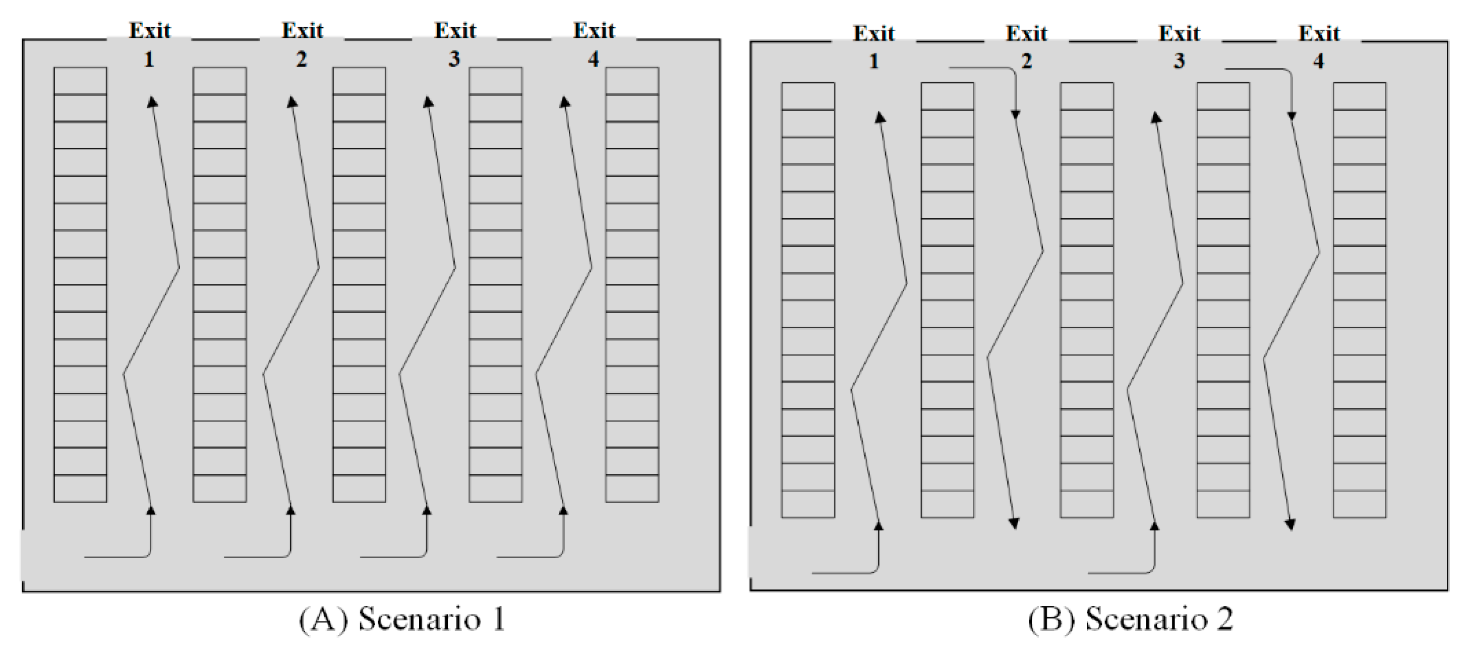
As can be seen in Figure 12, the first scenario, called $E_1$, is defined as a dedicated assignment in “Perchas” locations and by randomized classes in racks. Said randomness is determined by aisles, that is, a family that requires more than one aisle can randomly assign subfamilies among these, without losing the priority of the lightest at the beginning of the aisle and the heaviest at the end. In this way, the Subfamily Layout is built, which begins at the end of each aisle, where every two locations are filled on one side and pass to the other side of the aisle until all are completed. The second scenario, called $E_2$, corresponds to a dedicated allocation in “Perchas” locations and purely by classes in racks. The allocation by product family determines sequentiality in the aisles, that is, for a family that requires more than one aisle, it will not assign a subfamily $S_1$ until the subfamily $S_2$ has been assigned, always considering the stackability priority. Thus, the Subfamily Layout is built from the end of an aisle and the beginning of the next, where, as in $E_2$, the corridors are filled every 2 locations on one side and pass to the other side of the aisle, until all are completed.

The evaluation of each scenario is carried out considering the following criteria, in the

Table 6. Slotting scenario evaluation rubric, where the minimum score corresponds to 1 and the maximum score is 4.

Criteria	[%]	4	3	2	1
Total Distance Full pallet output distance Conformed pallet output distance Replenishment entry distance	$70$	Reduced over $10\%$ versus the base scenario.	Reduced between 5–10% versus the base scenario.	Reduced between 1–5% versus the base scenario	Does not reduce the distance versus the base scenario
Movement costs Use of cranes for a complete pallet Use of cranes for conformed pallets Use of cranes for replenishments	$30$	Reduced over $10\%$ versus base scenario	Reduced between 5–10% versus the base scenario	Reduced between 1–5% versus the base scenario	Does not reduce the costs versus base scenario

, based on a high sales day, called $V_{high}$, corresponding to period 2. $V_{high}$ has a set of trucks where each of them dispatches between one to four loads.

The number of full pallets that are dispatched is calculated from the number of total boxes requested in $V_{high}$ over the number of boxes per pallet of each SKU, then the distance traveled from the SKU location to the exit, multiplied by the number of movements, corresponds to the exit distance of complete pallets. Thus, everything that does not leave the warehouse as a complete pallet is collected per unit of boxes, which represents the exit distance of the conformed pallet. Replenishment comes from movements that deplete the availability of a pallet of SKUs in the warehouse. This calculation is determined by the number of times a position is empty when removing full pallets and/or boxes. Therefore, the route from entering the warehouse to a depleted position multiplied by the number of times it needs to be filled corresponds to the input distance for replenishment. Finally, the total distance arises from the aggregation of these three items. The above is summarized in Equation (35):

$$Total Distance={\displaystyle \sum }_c{\displaystyle \sum }_{ca}[P_i\left(d_S\right) +P{P}_i\left(d_S\right)] +R_i\left(d_E\right)$$

(35)

On the other hand, the cost criterion assesses the use of cranes based on the distances traveled for each defined operation, namely: cranes for a complete pallet, collection cranes, and replenishment cranes, as well as required operators. Average speed is defined in the Picking operation for cranes, considering high congestion, of $5 \mathrm{km}/\mathrm{h}$, where these have $6.5$ h of average use per operator and work shift. Each crane consumes approximately $11.13 \mathrm{Kwh}$, which is equivalent to $0.11 \mathrm{USD}/\mathrm{Kwh}$ (the data used for the accounting of operators and cranes are provided by the company). Besides, an average salary of $708.78 \mathrm{USD}$ per operator is considered [26]. Thus, the calculation of the number of operators necessary for the picking process by salary, added to the number of cranes by the value of electricity consumption and monthly rent, allows obtaining the total monthly cost, as indicated in Equation (36):

$$Movement costs=\left(W_{ps}+W_{pc}+W_{pe}\right)·Salary+\left(G_{ps}+G_{pc}+G_{pe}\right)A{\omega }_1{\omega }_2$$

(36)

8. Results

8.1. Computational Results

The algorithms were coded in Python, and the results were carried out on an Intel Core i5-8250U CUP 1.60 GHz 1.80 GHz core with 4 GB RAM.

Table 7. Computational results for the general subproblems of $P_1$.

Model	$\mathbf{Solver} \mathbf{Application} \left[\mathbf{sg}\right]$	$\mathbf{Results} \mathbf{Time} \left[\mathbf{sg}\right]$
$P_{1.1}$	$28.43$	$0.29$
$P_{1.4}$	$0.54$	$0.15$

shows the execution time and results for subproblems $P_{1.1}$ and $P_{1.4}$, while

Table 8. Computational results of the $P_1$ model for each scenario.

Model	Scenario	$\mathbf{Solver} \mathbf{Application} \left[\mathbf{sg}\right]$	$\mathbf{Results} \mathbf{Time} \left[\mathbf{sg}\right]$
$P_1$	$E_1$	$158.06$	$15.68$
$P_1$	$E_2$	$137.28$	$16.75$

provides duration time and results for each scenario evaluated. Complementary, the Execution Times with Gurobi’s Python Interface are presented in Appendix B.

Table 9. Computational results of the $P_{1.3}$ model for each scenario according to the evaluation family.

Family	Scenario	$\mathbf{Solver} \mathbf{Application} \left[\mathit{s}\mathit{g}\right]$	$\mathbf{Results} \mathbf{Time} \left[\mathit{s}\mathit{g}\right]$
Family 1	$E_1$	$0.05$	$0.19$
Family 3	$E_1$	$0.53$	$1.47$
Family 7	$E_1$	$0.09$	$1.80$
Family 1	$E_2$	$0.05$	$0.15$
Family 3	$E_2$	$2.59$	$0.60$
Family 7	$E_2$	$0.78$	$0.25$

shows the execution time and results for subproblems $P_{1.3}$, considering scenarios and family.

8.2. Results by Subproblems

For subproblem $P_{1.1}$, the minimum number of locations to be divided corresponds to $16.17\%$ of the total locations, a value that includes $24.14\%$ locations with double position and $75.86\%$ with a triple position.

Table 10. Corresponding percentages of the total locations available in the defined warehouse by family and subfamily.

Family	Total [%]	Subfamily	Simple Locations [%]	Double Locations [%]	Triple Locations [%]	Total [%]
Family 1	$6.23$	$s_1$	$0.00$	$0.19$	$0.56$	$0.74$
		$s_2$	$2.97$	$0.00$	$1.12$	$4.09$
		$s_3$	$0.00$	$0.00$	$0.19$	$0.19$
		$s_4$	$0.00$	$0.00$	$0.19$	$0.19$
		$s_5$	$0.28$	$0.00$	$0.19$	$0.46$
		$s_6$	$0.37$	$0.00$	$0.19$	$0.56$
Family 2	$2.79$	$s_1$	$0.09$	$0.19$	$0.37$	$0.65$
		$s_2$	$0.46$	$0.37$	$0.56$	$1.39$
		$s_3$	$0.19$	$0.00$.	$0.56$	$0.74$
Fily 3	$70.72$	$s_1$	$1.86$	$0.00$	$0.19$	$2.04$
		$s_2$	$30.67$	$0.56$	$1.12$	$32.34$
		$s_3$	$5.86$	$0.56$	$0.56$	$6.97$
		$s_4$	$0.74$	$0.00$	$0.74$	$1.49$
		$s_5$	$12.55$	$0.00$	$0.37$	$12.92$
		$s_6$	$13.29$	$0.74$	$0.93$	14.96
Family 4	$3.72$	$s_1$	$0.00$	$0.19$	$0.19$	0.37
		$s_2$	$0.09$	$0.19$	$0.19$	0.46
		$s_3$	$0.56$	$0.00$	$0.00$	0.56
		$s_4$	$0.56$	$0.00$	$0.19$	0.74
		$s_5$	$1.21$	$0.19$	$0.19$	1.58
Family 5	$0.74$	$s_1$	$0.37$	$0.19$	$0.19$	0.74
Family 6	$2.23$	$s_1$	$1.30$	$0.19$	$0.74$	2.23
Family 7	$13.57$	$s_1$	$0.37$	$0.19$	$0.19$	0.74
		$s_2$	$8.55$	$0.19$	$2.23$	10.97
		$s_3$	$1.49$	$0.00$	$0.37$	1.86

shows the number of locations for each family and subfamily, in which the latter is described by the set $S$ with index $\epsilon$, where $\epsilon$ indicates the number of regrouping of a family.

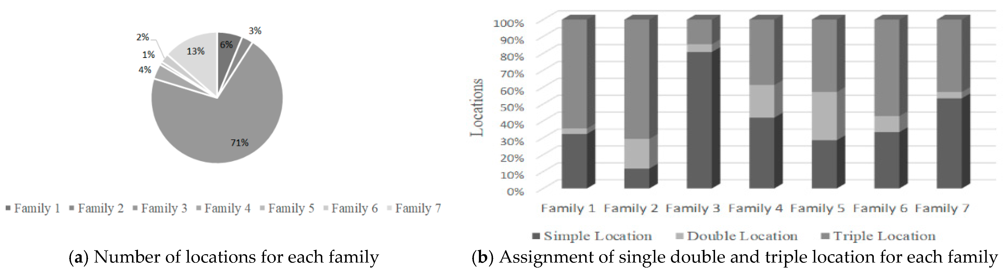
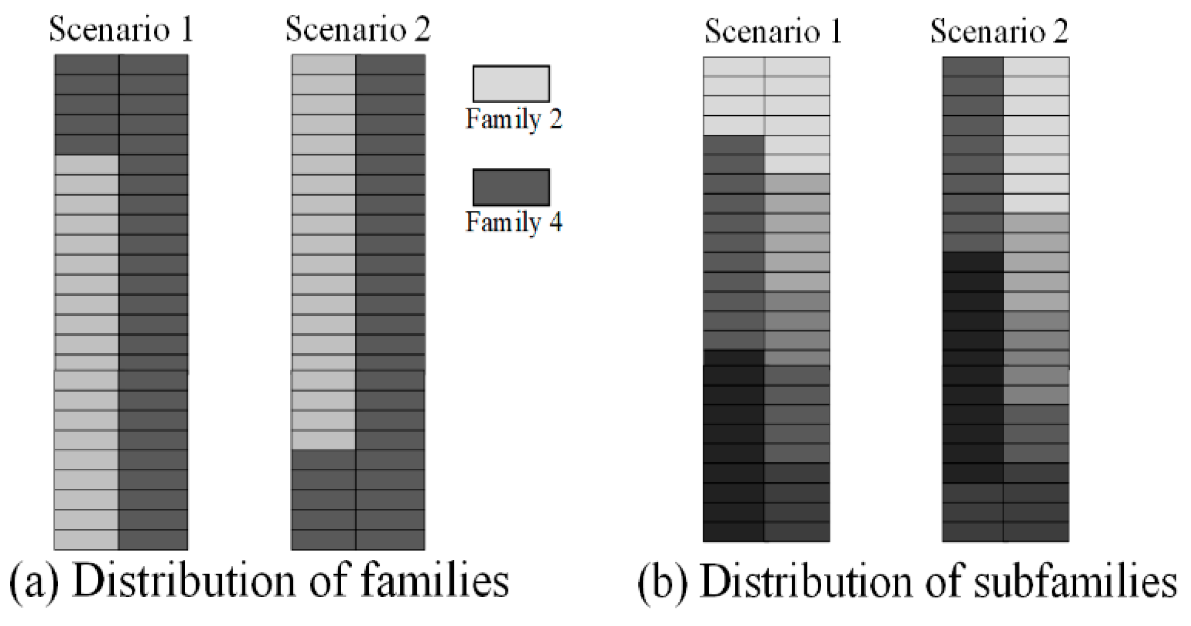
From Figure 13, it is possible to notice that the largest number of locations belongs to family 3, which has the highest percentage of simple locations. This fact reveals that this family is the most requested during this period. On the contrary, family 2 represents the highest percentage of triple locations, from which it can be concluded that this family contains mostly SKUs of type “B” and “C”.

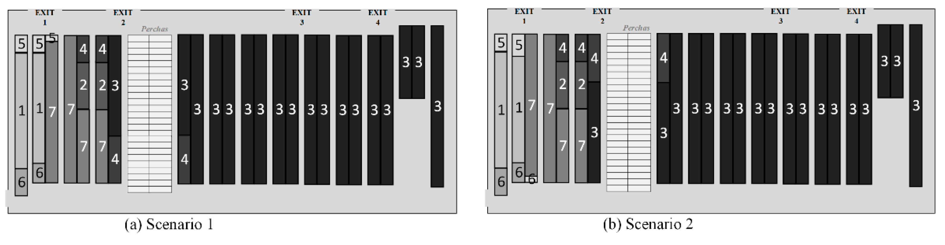
For the subproblem $P_{1.2}$, the design of the distribution of families per aisle follows the order described in Figure 14 and Figure 15, where they are assigned into the warehouse from left to right. Furthermore, the described configuration considers the results obtained in $P_{1.1}$ and the relationship generated in Figure 9.

The difference between both scenarios is highly observable in the distribution by subfamily, specifically in the right section of the warehouse, since it corresponds to the assignment of the largest family in SKUs covering the largest number of aisles, as can be seen in Figure 15. The gradient color (from light to dark) represents from lower to higher weight by subfamilies.

On the other hand, the division of locations is represented in Figure 16a and Figure 17a, where the execution of the model $P_{1.3}$, reveals that the divided locations should be applied to the end of each aisle, while the simple ones should be considered at the beginning. However, the stackability priority motivates a reorder within each aisle, without changing the family layout (see Figure 16b and Figure 17b).

Simple locations correspond mainly to type “A” SKUs, representing $86.6\%$ of the total of these locations, while double and triple locations mainly represent type “C” with SKUs $76.19\%$ and $76.52\%$, respectively. The rest are assigned for SKUs of type “B”.

Finally, the solution obtained in $P_{1.4}$ is observed in

Table 11. Corresponding percentages of the total Perchas locations available in the warehouse defined by family and subfamilies.

Family	$\mathbf{Total} \left[\mathit{\%}\right]$	Subfamily	$\mathbf{Total} \left[\mathit{\%}\right]$
Family 2	$45.74$	$S_1$	$24.47$
		$S_2$	$21.28$
Family 4	$54.26$	$S_1$	$5.32$
		$S_2$	$6.38$
		$S_3$	$9.57$
		$S_4$	$14.89$
		$S_5$	$18.09$

, as in the subproblem $P_{1.1}$, the number of locations for each family and subfamily is shown, where the latter is described by the set $S$ with indices $\epsilon$, where $\epsilon$ indicates the number of regroups in a family.

From these results, the distribution of families can be seen in Figure 18 for each scenario.

Finally, each previous result allows obtaining the SLAP-VH solution, that is, assigning at least one storage location to each SKU. According to this, the warehouse is increased due to the divided locations by $18.17\%.$

9. Results by Scenarios

The number of SKUs under the case study corresponds to $56.55\%$ of the SKUs $V_{high}$, where the rest belongs to the values warehouse, storage of merchandise of high monetary value that is normally sold for the minimum unit. Thus, based on the evaluation criteria described, $E_1$ scores $2$, while $E_2$ scores $1$. As can be seen in the

Table 12. Evaluation of Slotting scenarios based on the criteria defined in the rubric.

Criteria	${\mathit{E}}_1$	${\mathit{E}}_2$
	$\left[\mathrm{km}\right]$	$\left[\mathrm{km}\right]$
Total distance	$1792.38$	$1875.48$
Full pallet output distance	$36.63$	$39.78$
Conformed pallet output distance	$1706.41$	$1788.84$
Replenishment entry distance	$49.34$	$46.86$
Total	$3535.42$	$3750.96$
	$\left[\$\mathrm{USD}\right]$	$\left[\$\mathrm{USD}\right]$
Movement costs	$\mathrm{73,582.70}$	$\mathrm{76,559.99}$
Use of cranes for complete pallets	$\mathrm{12,754.34}$	$\mathrm{12,760.00}$
Use of cranes for conformed pallets	$\mathrm{51,998.44}$	$\mathrm{54,966.15}$
Use of cranes for replenishments	$8829.92$	$8833.85$
Total	$\mathrm{147,168.4}$	$\mathrm{153,159.99}$

.

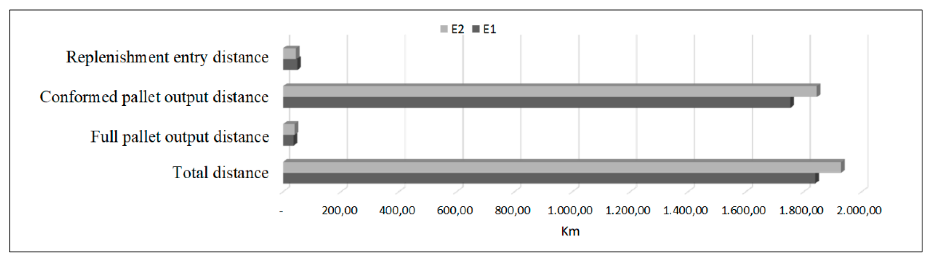
Regarding the minimum total distance for both scenarios, it is possible to observe, from Table 9, that the number of complete pallets is closer to the exit than those pallets that are conformed on the collection. However, the total exit distance is less in $E_1$. The distance to the entrance, represented by the replenishment pallet path, is closer for $E_2$, this indicates that those locations that run out of availability are closer to the reserve warehouse than in $E_1$. Thus, the total distance (input and output) is reduced by $4.64\%$ in $E_1$ with respect to $E_2$, as seen in Figure 19. Therefore, it can be stated that the most demanded SKUs are those closest to the exit on stage $E_1$. The preparation time is reduced in the same proportion, approximately 5%, since the time and the distance are directly proportional, but both are inversely proportional to the order in the warehouse, that is, the higher the order obtained, the lower is the distance traveled by the cranes and thus less time is spent on this item, clarifying that the calculated time does not consider the specific time between the loading or leaving a pallet at a location, this is purely the perspective of horizontal movement from one point to another.

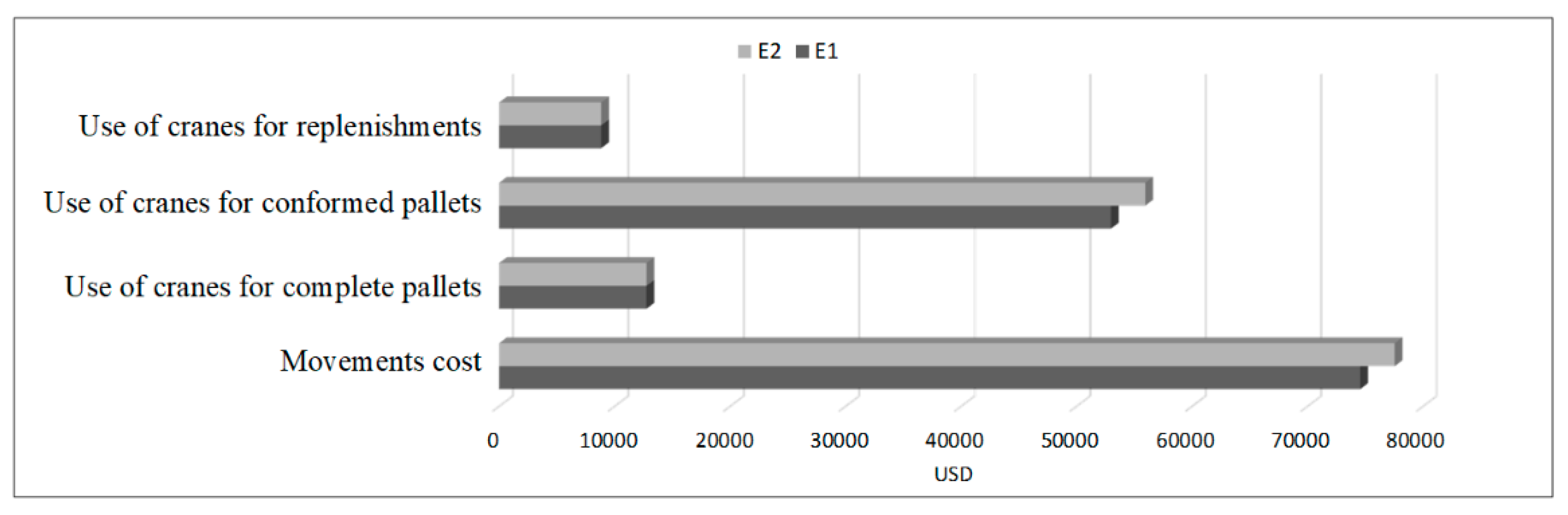
Finally, $E_1$ saves $4.05\%$ compared to $E_2$ in movement costs. Although the number of operators and cranes for full pallet picking and replenishment turn out to be similar since the distances traveled are similar, the greatest difference is observed in conformed pallets, where the number of operators, and therefore cranes, increases for $E_2$, since the travel time for this scenario corresponds to $5.19\%$ more than $E_1$, considering only the outbound route (pallet loading and unloading times are not included).

From the above it is possible to conclude that the dedicated and randomized storage strategy by classes allows reducing the route for cranes in the Picking process, achieving a cost reduction evaluated at 4% per month for this period of the study cycle as presented in Figure 20. Although the preparation of the best scenario requires greater precision, just by defining a better location for each SKU, this fact directly impacts the trip that the operator makes during Picking. The quantity required for each scenario with respect to the exit of the complete pallet and entry of the replenishment pallet turns out to be the same, given the movements that must be carried out and the defined route. However, the quantity in the unit collection varies significantly, being favorable for $E_1$, where not only the distance is reduced, but also the crane congestion is reduced since it requires a smaller number of operators than in $E_2$.

On the other hand, in both scenarios, the operation reports benefits due to the maximum use of the warehouse (considering the first level storage locations). However, the first scenario generates more advantages, such as better handling, avoiding damage to the products thanks to the priority of stackability. Most in-demand SKUs are closer to the exit, which means faster dispatching, facilitating the delivery process. Finally, distributing the products intelligently in the warehouse clears the aisles and facilitates the transfer of pallets both for the cranes that leave and those that enter to restock.

10. Discussion

Considering those authors who propose different ways of approaching the Slotting optimization problem, the vast majority of these focus on solving it through metaheuristics based on search and accommodation placement. However, this study is carried out under a decomposition of the problem that determines each key decision. While decomposition is one of the optimal methods for tackling problems with broad key decisions, separating the problem allows greater handling of data manipulation and a dedicated focus on each decision to be resolved. The computational results reveal the impact on the flow time of the executions for each subproblem and at the same time for each scenario, where each model provides the necessary data to address the problem in a sequential method and additional information that allows generating an effective analysis of each subproblem which helps to create a faster and better result in the SLAP-VH solution procedure. Ref. [1] analyzed the efficiency between solving the assignment problem metaheuristically and mathematically, where the latter does not turn out to be very fast in terms of the average execution time ($\mathrm{26,640}$ s, while the heuristic algorithm took $155$ s). However, it provides a solution that is very close to optimal, where the mean gap of the solutions is 4.3% after excluding an outlier.

This study groups each factor of the Slotting design to improve the Picking operation, such as distance, cost of operation, crane movements, use of human resources, and storage strategies based on implementation alternatives. Although the studies carried out by other authors evaluate the application of the methodology, the results obtained before the application are similar when using both decomposition and a metaheuristic. Comparing the result obtained by [14] which obtains a 4% reduction in the cost of human resources considering the departure of a specific batch of accommodation, the same percentage was obtained in the reduction of costs for accommodation in first level locations corresponding to the SLAP-VH problem. In addition, Slotting has been applied in the same way as in each of the compared investigations, where the methodology used is the same, but the impact depends completely on the storage space since it is not the same case to apply a Slotting optimization in a maritime terminal [11] versus a beverage distribution center. As for the infrastructure, the handling of the type of material, and, most importantly, the specific objective of performing the Slotting. For example, the results obtained by [12] are related to the objective of programming and assigning cranes, according to their specifications, to carry out operations in the locations where they can work. While for this study, the results obtained are related to improving the picking process and reducing the distance of cranes.

Finally, the solution to the problem will depend on four major factors: the storage location type, the storage strategy, the number of SKUs to be stored, and the warehouse’s size. All these factors are strongly related when it comes to minimizing travel time, operational cost, and storage usage. The model used in this research connects these factors considering divisible locations in racks and “Percha” locations, the two storage strategies evaluated in the different scenarios, families, subfamilies and SKUs, and the warehouse entry/exit distance. Comparing the different scenarios, $E_1$ exceeded $E_2$ in terms of the quality of the solution and the computational time optimally, significantly improving the distance traveled by the cranes and, simultaneously, the warehouse space usage as well as the operating cost.

11. Conclusions and Summary

The proposed research developed the SLAP-VH problem, which was decomposed into four subproblems of mathematical modeling solved sequentially in a storage environment of variable height and floor locations, where each one covered a key decision to achieve the proposed general objective. The results of the evaluation of the Slotting scenarios are alternatives that seek to approach the main problem in the Picking operation: the unproductive travel time during the pallet transfers by the cranes in order preparation. The application of this model allows defining the best location for each SKU, considering that the appropriate allocation strategy for the size of the study warehouse corresponds to $E_1$. According to the results of the case study, there is a decrease in the distance traveled of 5% of $E_1$ with respect to $E_2$.

On the other hand, the benefits granted by the best scenario are reflected in the maximum utilization of the warehouse, since the products are assigned efficiently, avoiding their deterioration due to the priority of stackability. In addition, this strategy improves the use of human resources and vehicles in the operation, the workload distribution, and also reduces the operating costs. The results obtained from the research provide valuable information for managers, where they can define, according to their warehouse capacity and the ABC classification of their SKUs, the intelligent allocation of each product within the warehouse. In parallel, minimizing the number of trips made in order to reduce the distance of travel of cranes by optimizing Slotting, is equivalent to reducing the number of operators, a favorable strategy for operating costs.

The solution design can be adapted and applied to other similar storage systems, modifying four main input parameters: warehouse capacity, demand for SKUs, incorporation of families, and the proper distances to evaluate, where the objective function used could be further enriched by including the picking routes, creating a combination of studies between the best Picking route and the slotting optimization.

References

- Öztürkoğlu, Ö. A bi-objective mathematical model for product allocation in block stacking warehouses. Int. Trans. Oper. Res. 2017, 27, 2184–2210. [Google Scholar] [CrossRef]
- Bartholdi, J.; Hackman, S. Warehouse and Distribution Science; 2014; Available online: http://www2.isye.gatech.edu/~jjb/wh/book/editions/wh-sci-0.96.pdf (accessed on 1 December 2020).
- Frazelle, E. Chapter 9: Logistics and Supply Chain Information Systems. In Supply Chain Strategy: The Logistics of Supply Chain Management; McGraw-Hill: New York, NY, USA, 2002; p. 287. [Google Scholar]
- Manzini, R. (Ed.) Warehousing in the Global Supply Chain. Advanced Models, Tools and Applications for Storage Systems; Springer: London, UK, 2012. [Google Scholar] [CrossRef]
- Yang, L.; Liu, W. The Study of Warehousing Slotting Optimization Based on the Improved Adaptive Genetic Algorithm. In Proceedings of the 6th International Conference on Advanced Materials and Computer Science (ICAMCS 2017), Zhengzhou, China, 29–30 April 2017. [Google Scholar] [CrossRef]
- Petersen, C.G.; Siu, C.; Heiser, D.R. Improving order picking performance utilizing slotting and golden zone storage. Int. J. Oper. Prod. Manag. 2005, 25, 997–1012. [Google Scholar] [CrossRef]
- Hompel, M.; Schmidt, T. Chapter 1: Introduction. In Warehouse Management: Automation and Organisation of Warehouse and Order Picking Systems; Springer: Heidelberg/Berlin, Germany, 2007; pp. 1–12. [Google Scholar] [CrossRef]
- Lorenc, A.; Lerher, T. Effectiveness of product storage policy according to classification criteria and warehouse size. FME Trans. 2019, 47, 142–150. [Google Scholar] [CrossRef]
- Ai-Min, D.; Jia, C. Research on slotting optimization in automated warehouse of pharmaceutical logistics center. Int. Conf. Manag. Sci. Eng. Annu. Conf. Proc. 2011, 135–139. [Google Scholar] [CrossRef]
- Van den Berg, J.; Gademann, A.J.R.M. Optimal routing in an automated storage/retrieval system with dedicated storage. IIE Trans. (Inst. Ind. Eng.) 1999, 31, 407–415. [Google Scholar] [CrossRef]
- Chen, L.; Lu, Z. The storage location assignment problem for outbound containers in a maritime terminal. Int. J. Prod. Econ. 2012, 135, 73–80. [Google Scholar] [CrossRef]
- Ballestín, F.; Pérez, Á.; Quintanilla, S. A multistage heuristic for storage and retrieval problems in a warehouse with random storage. Int. Trans. Oper. Res. 2017, 27, 1699–1728. [Google Scholar] [CrossRef]
- Park, C.; Seo, J. Mathematical modeling and solving procedure of the planar storage location assignment problem. Comput. Ind. Eng. 2009, 57, 1062–1071. [Google Scholar] [CrossRef]
- Gómez, R.; Cano, J.; Campo, E. Gestión de la asignación de posiciones (Slotting) eficiente en centros de distribución agroindustriales. Espacios 2018, 39, 23. [Google Scholar]
- Li, H.P.; Fang, Z.F.; Ji, S.Y. Research on the slotting optimization of automated stereoscopic warehouse based on discrete particle swarm optimization. In Proceedings of the 2010 IEEE 17th International Conference on Industrial Engineering and Engineering Management, IE and EM2010, Xiamen, China, 29–31 October 2010; pp. 1404–1407. [Google Scholar] [CrossRef]
- Damodaran, P.; Koli, S.; Srihari, K.; Kimler, B. Optimal product slotting. In Proceedings of the IIE Annual Conference, Norcross, GA, USA, 14–18 May 2005; pp. 1–6. [Google Scholar]
- Mantel, R.J.; Schuur, P.C.; Heragu, S.S. Order oriented slotting: A new assignment strategy for warehouses. Eur. J. Ind. Eng. 2007, 1, 301–316. [Google Scholar] [CrossRef]
- Kasemset, C.; Meesuk, P. Storage Location Assignment Considering Three-Axis Traveling Distance: A Mathematical Model. In Logistics Operations, Supply Chain Management and Sustainability; Golinska, P., Ed.; Springer: Cham, Switzerland, 2014; pp. 15–30. [Google Scholar] [CrossRef]
- Lerher, T. Travel time model for double-deep shuttle-based storage and retrieval systems. Int. J. Prod. Res. 2015, 54, 2519–2540. [Google Scholar] [CrossRef]
- Wisittipanich, W.; Kasemset, C. Metaheuristics for warehouse storage location assignment problems. Chiang Mai Univ. J. Nat. Sci. 2015, 14, 361–377. [Google Scholar] [CrossRef] [Green Version]
- Gómez, R.A.; Giraldo, O.G.; Campo, E.A. Conformación de Lotes Mínimo Tiempo en la Operación de Acomodo Considerando k Equipos Homogéneos usando Metaheurísticos. Inf. Tecnol. 2016, 27, 53–62. [Google Scholar] [CrossRef] [Green Version]
- Bahrami, B.; Aghezzaf, E.H.; Limère, V. Enhancing the order picking process through a new storage assignment strategy in forward-reserve area. Int. J. Prod. Res. 2019, 57, 6593–6614. [Google Scholar] [CrossRef]
- Lorenc, A.; Lerhet, T. PickupSimulo–Prototype of Intelligent Software to Support Warehouse Managers Decisions for Product Allocation Problem. Appl. Sci. 2020, 10, 8683. [Google Scholar] [CrossRef]
- Lorenc, A.; Kuznar, M.; Lerher, T. Solving Product Allocation Problem (PAP) by Using ANN and Clustering. FME Trans. 2021, 49, 206–213. [Google Scholar] [CrossRef]
- Zäpfel, G.; Wasner, M. Warehouse sequencing in the steel supply chain as a generalized job shop model. Int. J. Prod. Econ. 2006, 104, 482–501. [Google Scholar] [CrossRef]
- BNE. Bolsa Nacional de Empleo. 2020. Available online: https://www.bne.cl/ (accessed on 1 December 2020).
Figure 1.
Representation of a divisible location of the first level of variable height accommodation. Where , and correspond to the maximum, half the maximum height, and minimum height respectively.
Figure 2.
Definition of periods for SLAP-VH based on the monthly demand of each SKU grouped by families.
Figure 3.
Layout of the study distribution center. The lighter slots represent Perchas, while the darker slots are racks.
Figure 4.
Representation of Perchas locations with a two-sided view, where each rectangle represents an SKU pallet. Bold arrows indicate pallet entry.
Figure 5.
Representation of the first accommodation level locations with simple, double, and triple division, where (a.1), (b.1), and (c.1) correspond to the front view of a storage location in a rack, while (a.2), (b.2), and (c.2) correspond to the side view. Bold arrows indicate pallet entry.
Figure 6.
Solution framework for the study problem.
Figure 7.
Representation of Percha location, ordered with five base pallets and three levels.
Figure 8.
General flow diagram for resolution model of the SLAP-VH study problem.
Figure 9.
Classification diagram by affinity.
Figure 10.
The fusion between the affinity classification diagram and the store. The numbers indicate the families positioned by racks in each aisle.
Figure 11.
Assignment problem diagram .
Figure 12.
Representation of the filling sequence.
Figure 13.
Percentage representation for the results obtained in .
Figure 14.
Representation of the family layout in the study warehouse for . The gray variation corresponds in (a) for each family and in (b) for each subfamily.
Figure 15.
Figure 16.
Layout of types of location in the warehouse, where (a) corresponds to the execution of for and (b) to the reorder by stackability.
Figure 17.
Figure 18.
Families layout in Perchas location corresponding to sides with non-divisible locations.
Figure 19.
Variation between both scenarios regarding the total distance criterion.
Figure 20.
Variation between both scenarios with respect to the cost of movements criterion.